BOUNDED ORDERED SETS BY PRINCIPAL LATTICE CONGRUENCES
G ´ABOR CZ ´EDLI
Abstract. For bounded lattices L1 andL2, let f:L1 → L2 be a lattice homomorphism. Then the map Princ(f) : Princ(L1)→Princ(L2), defined by con(x, y)7→con(f(x), f(y)), is a 0-preserving isotone map from the bounded ordered set Princ(L1) of principal congruences ofL1to that ofL2. We prove that every 0-preserving isotone map between two bounded ordered sets can be represented in this way. Our result generalizes a 2016 result of G. Gr¨atzer from{0,1}-preserving isotone maps to 0-preserving isotone maps.
1. Introduction and our result
We assume that the reader has some familiarity with lattices and their congru- ences; if not then Gr¨atzer [13, 19] and the freely down-loadable Nation [33] are recommended. Postponing some details about our motivation and a short survey of related results to Section 2, here we are going to get to our result in a short way.
For a latticeL, let Princ(L) =hPrinc(L);⊆i denote theordered set of principal congruences of L. A congruence of L is principal if it is of the form con(a, b) = conL(a, b) for some elements a, b ∈ L, that is, if it is generated by a single pair ha, bi. IfL is bounded, which means that 0,1∈ L, then so is Princ(L). In 2013, Gr¨atzer [14] proved the converse: up to isomorphism, every bounded ordered set is of the form Princ(L) whereLis a bounded lattice. Since no similar characterization is known for non-bounded ordered sets in general, we study the representability of isotone maps by principal lattice congruences only among bounded ordered sets.
For bounded latticesL1, L2and a lattice homomorphismg:L1→L2, it is natural to consider the map
(1.1) Princ(g) : Princ(L1)→Princ(L2), defined by conL1(x, y)7→conL2(g(x), g(y)).
It was observed by Gr¨atzer [20] that (1.1) defines indeed a map, since one can easily show that conL1(x1, y1) = conL1(x2, y2) implies that conL2(g(x1), g(y1)) = conL2(g(x2), g(y2)). Clearly, the map Princ(g) is 0-preserving and isotone. The following definition is quite natural; analogous concepts have been used for (not necessarily principal) congruences in several earlier papers including Cz´edli [1] and Gr¨atzer [20].
2000Mathematics Subject Classification. 06B10, 18B05. Oct 8, 2017,revised April 30, 2018.
Key words and phrases. Principal congruence, lattice congruence, ordered set, poset, quasi- colored lattice, preordering, quasiordering, isotone map, representation.
This research was supported by NFSR of Hungary (OTKA), grant number K 115518.
1
Definition 1.1. Letf:P1→P2be a 0-preserving isotone map from an ordered set P1with 0 to an ordered set P2 with 0. We say thatf isrepresentable by principal congruences of bounded latticesif there exist latticesL1andL2, order isomorphisms hi: Pi →Princ(Li), for i∈ {1,2}, and a lattice homomorphismg:L1 →L2 such thatf =h−12 ◦Princ(g)◦h1, that is, the diagram
(1.2)
hP1;≤P1i f
−−−−→ hP2;≤P2i h1
y h−12
x
hPrinc(L1);⊆i Princ(g)
−−−−−−→ hPrinc(L2);⊆i
is commutative. If we can find lattices L1 and L2 of lengths at most m and n, respectively, such that (1.2) holds, then we say that f isrepresentable by principal congruences of lattices of lengths at most m and n. We also say that the lattice homomorphism g representsf by means of principal congruences.
We say thatf in (1.2) is 0-separating, 1-preserving, and 0-preserving if we have that {x∈P1: f(x) = 0} ={0}, f(1) = 1, and f(0) = 0, respectively. Of course, the 1-preserving property assumes that bothP1 and P2 have largest elements. It was proved in Cz´edli [3] that iff has all the three properties listed above, then it is representable by principal congruences of bounded lattices. Later, Gr¨atzer [20]
proved that the first of the three conditions can be omitted, that is, whenever f in (1.2) is 0-preserving and 1-preserving, then it is representable by principal congruences of bounded lattices. Strengthening this result even further, our aim is the prove that the preservation of 0 in itself guarantees representability; this is formulated in our theorem below.
Theorem 1.2. If f:P1→P2is a0-preserving isotone map from a bounded ordered setP1=hP1;≤P1ito a bounded ordered setP2=hP2;≤P2i, thenf is representable by principal congruences of bounded lattices of lengths at most5 and 7.
Theorem 1.2 gives an affirmative answer to F. Wehrung’s question asked at the conference SSAOS-55, Nov´y Smokovec, Slovakia, 2017. Related results on ordered sets of principal congruences have recently been given in Cz´edli [3, 4, 6, 7, 9, 8], Gr¨atzer [14, 20, 21, 22, 23], and Gr¨atzer and Lakser [28, 29].
Remark 1.3. If none ofP1andP2is a singleton, then we can choseL1 andL2 in Theorem 1.2 such thatL1is of length 5 whileL2 is of length 7.
Outline. Section 2 contains a mini survey of earlier results that motivate our present work. The rest of the paper is devoted to the proof of Theorem 1.2 and Remark 1.3. Section 3 describes the construction we need; first in a pictorial and easy-to-understand way for a concrete example, and then we expand this visual description to a general construction. Section 4 verifies our construction, whereby the theorem follows. Also, Section 4 points out why Remark 1.3 holds.
2. Motivation and a mini survey
There are so many results on congruence lattices of lattices which motivate the present paper that this section, added on April 30, 2018, is restricted only to a mini survey of them. This short section and the list of the papers referenced here are far from being complete; a complete treatment would need a whole book. For much
more extensive and very deep surveys up to their publication dates, the reader is referred to the monograph Gr¨atzer [19] and to the book chapters Gr¨atzer [16] and [17] and Wehrung [37], [38], and [39].
By a well-known old result of Funayama and Nakayama [12], the lattice Con(L) = hCon(L);⊆i of all congruences of a latticeL is distributive. The converse for the finite case is due to R. P. Dilworth but, independently, it was first published in Gr¨atzer and Schmidt [30]. This result states that every finite distributive lattice is (isomorphic to) the congruence lattice Con(L) of a finite lattice L. In spite of several positive results, mile-stoned by Huhn [32] and Schmidt [35], which represent some infinite distributive algebraic lattices as congruence lattices of lattices; it was a real breakthrough when Wehrung [36] presented a distributive algebraic latticeD such thatD ∼= Con(L) holds for no latticeL. Later, such a distributive algebraic latticeDof minimal cardinality was given by R˚uˇziˇcka [34].
Compared to the infinite case, much more results have been proved on the rep- resentability of finite distributive latticesDby congruence lattices of finitelattices L. There are several results in which, in addition to D ∼= Con(L), the lattice L has some nice properties or its automorphism group is isomorphic to a given fi- nite group; we mention Gr¨atzer and Knapp [24] and Gr¨atzer and Schmidt [31] as some attracting examples of this sort. A homomorphismf:L1→L2 between two lattices naturally induces an isotone map from Con(L1) to Con(L2) or backwards, and various papers represent isotone maps between two finite distributive lattices in this way; see, for example, Gr¨atzer and Lakser [25]. Several papers do this so that the latticesL1 and L2 have some nice properties; see, for example, Cz´edli [1]
and Gr¨atzer and Lakser [26] and [27]. Instead of representing a single map, there is a whole theory of representing families of isotone maps; see Wehrung [39].
In a pioneering paper, Gr¨atzer [14] proved that every bounded ordered setP= hP;≤i is isomorphic to hPrinc(L);⊆i for some lattice L. This result naturally leads to the followinggeneral problem: find the “hP,Princ(L)i-type” counterparts of the “hD,Con(L)i-type” results mentioned so far in this section and, in addition, find analogous “hP ⊆D,Princ(L)⊆Con(L)i-type” representability results. Some concrete instances of this general problem are formulated at the end of Gr¨atzer [17].
The present paper is motivated by and contributes to the progress outlined in this section above and mentioned right after Theorem 1.2. In spite of this progress, the present paper, and the very recent Cz´edli and Mure¸san [11], we are far from the solution of the above-mentioned general problem.
3. The construction
3.1. Decomposing f. LetP1 andP2be bounded ordered sets. Assume that
(3.1)
f:P1 → P2 is a 0-preserving isotone map. Let P3 be the principal ideal of P2 generated by f(1P1), that is, P3 = ↓f(1P1). Then f decomposes as f = f3 ◦ f1, wheref1:P1→P3, defined byf1(x) :=f(x), is a{0,1}- preserving isotone map and f3: P3 → P2, defined by x7→x, is a 0-preserving injective isotone map.
Note that the embedding f3 is necessarily 0-separating. We can use Cz´edli [7]
to represent f1, while some ideas of Cz´edli [4] can be modified to represent f3. Finally, the composite of these two representations is what we need in order to prove Theorem 1.2. Since Cz´edli [4] and [7] are long papers and it would take a lot
of time of the reader to extract and appropriately modify ideas from them, we are going to outline these ideas by a concrete but sufficiently general example.
From now on, we denote the bottom element and the top element ofPiby 0iand 1i, respectively, while those ofLi will be denoted by the boldface symbols000i and 111i. When no ambiguity threatens, we will often writehPi,≤iiinstead ofhPi,≤Pii.
The least congruence and the largest congruence of a latticeLwill be denoted by
∆Land∇L, respectively. LetLbe an ordered set or a lattice. Forx, y∈L,hx, yiis called anordered pair ofLifx≤y. Ifycoversx, thenhx, yiis anedgeofL. Edges andprime intervals are essentially the same but edges are pairs of elements while prime intervals are two-element subsets. The set of ordered pairs ofL is denoted by Pairs≤(L). As opposed to the concept of intervals [x, y], pairs and the notation hx, yimake it clear thatS⊆Limplies that Pairs≤(S)⊆Pairs≤(L).
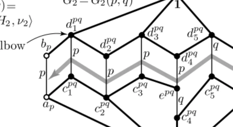
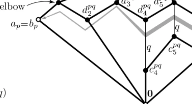
Figure 1. Our gadgetG2=G2(p, q) =hG2;γ2, H2, ν2i
3.2. Basic gadgets and their pictograms, the zigzag arrows. Our basic tool is the lattice G2 =G2(p, q) given on the right of Figure 1. This lattice is taken from Cz´edli [7], where it is denoted by Gup2(p, q), because [7] also uses its “down”
variant. Some details of Figure 1 that are not needed at this stage will be explained later. Note that we can use G2 and G2 with parameters other than pand q, and we often drop the parameters if they are not relevant or they are clear from the context. The edgeshaq, bqiandhap, bpiare called thefirst edgeand the target edge of G2(p, q), respectively. In order to make our figures less crowded, we will often denote G2 by a greyzigzag arrow that is directed from its first edge to its target edge. We also say that the zigzag arrowgoes fromthe first edgetothe target edge.
Sometimes we draw a double-lined zigzag arrow to indicate that besides a zigzag arrow some other elements (whose set will be denoted by Upq in our figures) are also added. We will explain later why we need double-lined zigzag arrows and we will define them exactly in (3.18); at present, it suffices to know that their role is the same as that of the “single-lined” zigzag arrows. Zigzag arrows without the adjective “double-lined” are always understood as single-lined ones. Observe that con(ap, bp) collapses only thep-labeled edges, so its non-singleton blocks are {ap, bp},{cpq1 , dpq1 },{cpq2 , dpq2 },{cpq3 , dpq3 }, and{epq, dpq4 }. Similarly,
(3.2) the non-singleton blocks of con(aq, bq) are{ap, bp},{cpq1 , dpq1 },{cpq2 , dpq2 }, {cpq3 , dpq3 },{cpq4 , epq, dpq4 },{cpq5 , dpq5 },{cpq6 , dpq6 }, and{aq, bq}.
The quotient lattices G1 := G2/con(ap, bp) and G0 := G2/con(aq, bq) and the corresponding “gadget structures” will be denoted by different kinds of grey zigzag arrow pictograms as Figures 2 and 3 show. These arrows will have no double-lined variants.
Figure 2. The quotient gadgetG1=G1(p, q) =hG1;γ1, H1, ν1i
Figure 3. The quotient gadgetG0=G0(p, q) =hG0;γ0, H0, ν0i
The zigzag arrow notation in Figure 1 and also in other figures is motivated by the way the congruences spread: con(aq, bq)≥ hap, bpi, that is, con(aq, bq) collapses thep-colored edgehap, bpi. The latticeG2 and its quotient latticesG1 andG0 will be referred to as ourgadgets orzigzag arrows. Sometimes,G1andG0will be called
“quotient zigzag arrows”. Note that
(3.3) con(ap, bp) and con(aq, bq) are the only nontrivial congruences ofG2(p, q),
whereby we will use only two kinds of quotient zigzag arrows. So, there are three different zigzag arrows, the “non-quotient” G2 and two quotient ones, G1 and G0. Now we premise our plans with them in our construction; this will hopefully help to enlighten the basic ideas, which will be detailed later. Note, however, that these plans will become more clear only in Subsection 3.3.
First, assume that we want to represent a single ordered set hP;≤Pi in the form hPrinc(L);⊆i. Then we have to find a lattice L and an order isomorphism h:hP;≤Pi → hPrinc(L);⊆i. It will be clear from Subsection 3.3 soon that, for p∈P, we will leth(p) := con(ap, bp). Also, forp < qinP, we will extend the set
(in fact, the six-element sublattice){0, ap, bp, aq, bq,1}to the zigzag arrowG2(p, q) of Figure 1; the reason is that the zigzag arrow
(3.4) G2(p, q) forces the inequality con(ap, bp)≤con(aq, bq),
and this inequality is needed to guarantee thathis isotone. We do not need quotient zigzag arrows for this purpose, because they force only that ∆L≤con(aq, bq) and
∆L≤∆L, which automatically hold. However, even if they are superfluous at this stage, quotient zigzag arrows can be included, since they do not disturb the job of the “non-quotient”G2 zigzag arrows.
Second, the situation becomes more involved when we want to represent the map f from (3.1) (with the subscript 2 changed to 3) from hP1;≤1i to hP3;≤3i.
We will represent hP1;≤1iby an order isomorphismh1:hP1;≤1i → hPrinc(L1);⊆i without quotient zigzag arrows as explained in the previous paragraph. But then we will face the problem that for 0 <1 p <1 q in P1, it may happen that, say, 03=f1(p)<3f1(q) inP3. Since f1 is intended to be represented as Princ(g1), see (1.1) (but replace the subscript 2 by 3), it follows from (1.2) (after slight notational changes) that
(3.5) ∆L3=h3(03) =h3(f1(p)) = Princ(g1)(h1(p))
= Princ(g1)(con(ap, bp)) = con(g1(ap), g1(bp)).
This means that g1 collapsesap and bp, that is, hap, bpi ∈ Ker(g1). On the other hand, a calculation similar to (3.5) shows thathaq, bqi∈/ Ker(g1). Hence, it follows from (3.3) thatg1maps theG2(p, q) sublattice ofL1 onto a quotient zigzag arrow G1. So even ifG1would not be necessary to representhP3;≤3iin itself, some copies ofG1has to be included inL3, because otherwise we could not define an appropriate lattice homomorphismg1:L1 → L3. The motivation for using G0 is similar but it has an additional feature. Namely, if 03 =f1(p) =f1(q), then Ker(g1) has to collapse each of the pairshap, bpiandhaq, bqi, but it cannot collapse a pair that is not collapsed by the congruence of G2(p, q) described in (3.2), because otherwise h0L1,1L1i would belong to Ker(g1) and Ker(g1) would collapse the whole lattice L1, so the range of Princ(g1) would be the singleton set {∆L3}, which is clearly not the case in general. Combining this with (3.3), it follows that g1 has to map G2(p, q) to a copy ofG0, provided that 03=f1(p) =f1(q).
Finally, the quotient zigzag arrows that are necessarily included in L3 will not disturb us to extendL3to a latticeL2 in a way similar to the one used in Cz´edli [4].
Figure 4. An example
3.3. Describing the construction with an example.
Example 3.1. LetP1={01, p, q, r,11} andP2={02, s, t, u, v,12} be the ordered sets given in Figure 4, and letf:P1→P2be the isotone map indicated by dashed arrows in the figure.
Figure 5 shows how we represent P1 as Princ(L1). We start with the eight element simple latticeM3,3; in Figure 5,M3,3is the sublattice ofL1formed by the pentagon-shaped elements. One of the edges of M3,3 that is disjoint from {0,1}
is denoted byha11, b11i; this edge and all thick edges in the figure are colored by 11∈P1. In the next step, we add the dark-grey-filled large elements. That is, for every x ∈ P1\ {01,11}, we add the thin edge hax, bxi. We often call this edge a basic edge. Our goal is that the principal congruence con(ax, bx) should represent x∈P1. That is, the map
(3.6) h1: P1→Princ(L1), defined by x7→con(ax, bx),
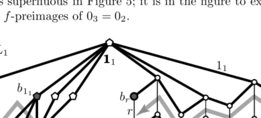
should be an order isomorphism. At present, we are far from this goal since the principal congruences con(ax, bx), for x∈P1\ {01,11}, form an antichain. There- fore, we add several copies of our gadgetG2 in order to force the comparability of con(ax, bx) and con(ay, by) whenever x, y ∈ L\ {01,11} are comparable. We can add a gadget going from the basic edgehay, byito the basic edgehax, bxifor every hx, yi ∈Pairs≤(P1\ {01,11}), but it is often sufficient to add less gadgets because of transitivity. Note that the gadget added to hp,11i, indicated only by a (thick grey) zigzag arrow, is superfluous in Figure 5; it is in the figure to exemplify later how to deal with thef-preimages of 03= 02.
Figure 5. P1∼= Princ(L1)
As Figure 6 shows, the representation ofP3=↓sas Princ(L3) is similar but we need some new features: L3has an extra elementa0(p)=b0(p), it has twos-colored thin basic edges, and there are gadgets, in both directions, between the s-colored basic edges. Also, to guarantee that thes-colored basic edges generate∇L3, a zigzag arrow goes from the basic edge has(q), bs(q)ito the edge ha13, b13i. Note that some edges ending at1113 or starting from0003need not indicate coverings in Figure 6; for example, since thet-colored basic edgehat, btiis the target edge of a zigzag arrow, we have only thatbt<1113 but bt ⊀1113. This will not cause any problem in what follows, and
(3.7) h3: P3→Princ(L3), defined by x7→con(ax, bx),
is an order isomorphism.
Figure 6. P3∼= Princ(L3)
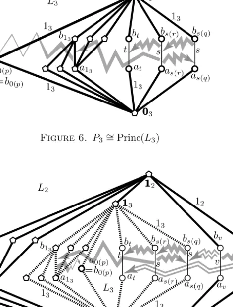
Figure 7. P2∼= Princ(L2)
The required homomorphismg1:L1→L3is defined as follows. It maps theM3,3
sublattice, which is the collection of the pentagon-shaped elements ofL1, onto the M3,3 sublattice of L3 such that g1(a11) = a13 and g1(b11) = b13. Motivated by f(p) = 03, f maps both ap and bp to a0(p) = b0(p). The element s ∈ P3 has two f-preimages in P1\ {11}; this explains that L3 has two s-colored thin basic edges. The pairs haq, bqi and har, bri are mapped to the pairs has(q), bs(q)i and has(r), bs(r)i, respectively. The left and the right grey zigzag arrows (representing copies ofG2) ofL1are mapped to the leftmost grey zigzag arrow and the rightmost upper zigzag arrow, respectively. SinceG1, the leftmost zigzag arrow in Figure 6, is a homomorphic image ofG2, it is easy to see that the mapg1we have just defined is a lattice homomorphism. It is straightforward to see, at least for Example 3.1, that
(3.8) g1 representsf1 by means of principal congruences;
see Definition 1.1. Note that since con(aq, ar) = ∇L1, it follows from (1.1) and f = Princ(g) that g(aq) 6= g(ar); this explains why we need two s-colored basic edges inL3. So far, we have not used any double-lined zigzag arrow.
As the last step of the construction, we extend L3 to a latticeL2 as shown in Figure 7. In this figure,L3 is the interval [0003,1113], and
(3.9) each of the thick dotted edges ofL3 generates a congruence that corresponds to 13∈P3.
In order to take care of the comparabilityu≤v, there is a new (single-lined) zigzag arrow in L2 with first edgehav, bvi and target edgehau, bui. (“New” means that it is not in L3.) This is possible because at the beginning, as previously, the top element bu of the target edge is a coatom in L2, so the new zigzag arrow lies in L2 basically in the same way as the zigzag arrows lied inL1 andL3. However, we use double-lined zigzag arrows inL2to take care of the comparabilitiess≤v and t≤u; we will explain later in (3.18) what these double-lined zigzag arrows are, and we will point out why a single-lined zigzag arrow cannot work if there is an edger in the filter generated by the top of its target edge such that con(r)6=∇L2.
Now that the new arrows, single-lined and double-lined, take care of each of the comparabilitiesu≤v,s≤v,t≤s, and t≤u, it follows that
(3.10) h2: P2→Princ(L2), defined by x7→con(ax, bx), is an order isomorphism. Letg3 be the natural embedding
(3.11) g3:L3→L2, defined by x7→x.
It is straightforward to see, at least for Example 3.1, that
(3.12) g3 representsf3 by means of principal congruences.
Let g = g3 ◦g1; it is a lattice homomorphism from L1 to L2. We know from Cz´edli [6, 7] and it is easy to see that Princ is a functor, whereby
(3.13) Princ(g3)◦Princ(g1) = Princ(g3◦g1) = Princ(g).
For i ∈ {1,3}, let hi: Pi → Princ(Li) denote the order isomorphism defined by x7→con(ax, bx); see (3.6), (3.7), and (3.10). By (1.2), (3.8) and (3.12) mean that (3.14) f1=h−13 ◦Princ(g1)◦h1 and f3=h−12 ◦Princ(g3)◦h3.
Combining (3.13) and (3.14), we obtain that
f =f3◦f1= (h−12 ◦Princ(g3)◦h3)◦(h−13 ◦Princ(g1)◦h1)
=h−12 ◦Princ(g3)◦Princ(g1)◦h1=h−12 ◦Princ(g)◦h1.
Hence, gis representable by principal congruences of lattices of lengths 5 and 7.
3.4. The construction for the general case. The construction for the general case is almost the same as that for Example 3.1. Hence, it suffices to point out the differences. The construction ofL1 is essentially the same as in the example.
For eachp∈f−1(02),L3has to contain an elementa0(p)=b0(p)that is an atom and also a coatom inL2. Remember that 02= 03. Of course,g1maps the elements ap andbp of L1 to the element a0(p) =b0(p) ∈L3. Note that forp, p0 ∈f−1(02), if p 6= p0, then a0(p) 6= a0(p0). For each s ∈ f(P1)\ {03}, we need as many s- colored thin basic edges in L3 as the size |f−1(s)\ {11}| of f−1(s)\ {11}. So if f−1(s)\ {11} ={q, r, . . .}, then we include the s-colored basic edgeshas(q), bs(q)i, has(r), bs(r)i, . . . inL3. In order to guarantee that every s-colored edge generates
the same congruence ofL3, we let a zigzag arrow go between any twos-colored basic edges in both directions. (Note that it often suffices to use fewer zigzag arrows; we only need that the “reflexive and transitive closure of the zigzag arrows” is the full relation on the set of s-colored edges ofL3.) So far, we have seen whatL3 is and we have defined the action ofg1for theM3,3sublattice ofL1 and for the thin basic edges ofL1.
In the next step, we extend the action of g1 to the gadgets. For each gadget, that is, for each zigzag arrowZ ∼=G2 ofL1, we do the following. Lethah, bhiand haw, bwibe the target edge and the first edge of Z, respectively, and observe that since Z is included inL1, we have thath≤1w inP1. Thus, f(h)≤3 f(w) in P3
since f is isotone, and there are three cases to consider.
First, if f maps none of h and w to 03, then hg1(ah), g1(bh)i = haf(h), bf(h)i andhg1(aw), g1(bw)i=haf(w), bf(w)iare basic edges ofL3andL3contains a zigzag arrowZ0 ∼=G2 fromhg1(aw), g1(bw)itohg1(ah), g1(bh)iby the construction ofL3. In this case, g1restricted toZ will be an isomorphism from Z toZ0.
Second, if f(h) = 03 6= f(w), then we modify L3 by adding a quotient zigzag arrow G1 that goes from hg1(aw), g1(bw)i = haf(w), bf(w)i to hg1(ah), g1(bh)i = ha0(h), b0(h)i. Observe thata0(h)=b0(h)and so con(a0(h), b0(h)) = ∆L3. Hence, the new zigzag arrow does not spoil the construction ofL3 since its only effect is to force the inequality ∆L3≤con(af(w), bf(w)), which holds automatically.
Third, iff(h) = 03=f(w), then we add a quotient zigzag arrowG0going from the “degenerate” (singleton) edgehg1(aw), g1(bw)i=ha0(w), b0(w)ito the degenerate edgehg1(ah), g1(bh)i=ha0(h), b0(h)i; this does not spoil anything.
Finally, we extendL3toL2and we defineg3in the same way as in Example 3.1.
SinceP3is a (principal) order ideal inP2, there are only two sorts of comparabilities u≤vinP2 that we still have to force, namely,
(3.15) either u, v∈P2\P3 andu≤v, or u∈P3 andv∈P2\P3 andu≤v.
In case of the first alternative mentioned in (3.15), every edgehx, yiwithx≥buis a thick and solid edge and generates the largest congruence; as a consequence to be clarified later, we use a (single-lined) zigzag arrow in this case. In the second case, we use a double-lined zigzag arrow; we are going to point out a few lines later why.
Note at this point that
(3.16) a zigzag arrow “arrives” at its target edge from above and “departs” from its first edge upwards;
see our figures. Therefore, as it will be explained later (with reference to the present paragraph), it needs a special attention whether all the edges above the target edge are thick and solid or not, but it is irrelevant whether the same holds below the target edge and below the first edge. As opposed to Cz´edli [4], now since all edges abovebv are thick and solid for both alternatives given in (3.15), the first edges of the new single-lined or double-lined zigzag arrows will need no special care.
Forp∈P3\ {03}, let
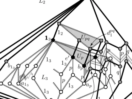
(3.17) Up:= [bp,1113], which is a filter inL3 and an interval inL2.
The elementdpq1 in Figure 1 will be called theelbow ofG2(p, q). By the construction ofL3,Up consists ofbp,1113, and the elbows of the zigzag arrows inL3 with target edgehap, bpi. (It may happen that there is no such elbow; then|Up|= 2. If|Up|>2, then it is a modular lattice of length 2.) Forp∈P3\ {03}andq∈P2\P3,inserting
a double-lined zigzag arrow with first edge haq, bqiand target edge hap, bpimeans that
(3.18)
first we insert a (single-lined) zigzag arrow, and then we add a new interval Upq isomorphic to Up such that [bp,1Upq] is isomorphic to the direct product of Up and the two-element chain{0,1}such thatUp corresponds toUp× {0}in [bp,1Upq];
see Figures 8 and 9 for illustration. In both figures, Up is the lowest grey-filled interval and it consists of the black-filled circles and the black-filled pentagon, while the intervalUpq is also grey-filled and it consists of the grey-filled square elements.
Figure 8. Up={black-filled elements}, a double-lined zigzag ar- row fromhaq, bqitohap, bpi, and a part ofL2(not for Example 3.1)
Note that (3.9) is still valid; in fact, our intention to preserve its validity explains why we cannot use (single-lined) zigzag arrows instead of double-lines ones here.
Namely, continuing the paragraph containing (3.16), remember that the bottom element of Upq is dpq1 , the elbow element of the zigzag arrow G2(p, q). Assume that we delete Upq\ {dpq1 } from Figure 8 or from Figure 9. Then the elbowdpq1 becomes a coatom andhdpq1 ,1112ibecomes a solid thick edge, that is, it generates the largest congruence ofL2 and so it corresponds to the top 12 ofP2. However, then the dotted thick edgehbp, e0iand the solid thick edgehdpq1 ,1112ibecome transposed, and so they generate the same congruence, which violates (3.9). Furthermore, it remains true that any two thick dotted edges generate the same congruence, and it turns out that no congruence of L2 corresponds to 13 ∈ P3; this is what we surely have to avoid. It will turn out that the usage of double-lined zigzag arrows is sufficient to keep the validity of (3.9), and ourL2 does the job.
As opposed to the top elementbp of the basic edge associated withp∈P3\ {03}, its bottom elementapdoes not cause a similar difficulty. So, as opposed toUpq in- serted above the single-lined partZof the double-lined zigzag arrow fromhaq, bqito hap, bpi, we do not have to add extra elements belowZ. In order to give a first im- pression why this is so, note that the ideal↓cpq1 ={0002,0003, ap, cpq2 , cpq1 }is a sublattice isomorphic toN5; see Figures 8 and 9. Obviously, the congruence con↓cpq
1 (0003, ap) generated by the dotted thick edge of this sublattice does not collapse any solid thick edge in this sublattice; much less obviously, the same will turn out to hold for conL2(0003, ap) in the whole latticeL2.
Figure 9. Adding the third double-lined zigzag arrow with target edgehap, bpiand a part ofL2 (not for Example 3.1)
4. Proving that our construction works
In this section, we are going to prove that our construction has the properties stated in Section 3; this will imply Theorem 1.2. A direct proof given in a self- contained way with all details would result in an extremely long paper, which we want to avoid. Therefore, we organize the proof so that it relies on very similar considerations, even if this makes it necessary to reference some long proofs in addition to some statements from earlier papers. First, we claim that (3.8) holds in general, not only for our example.
Lemma 4.1. The lattice homomorphism g1:L1→L3 constructed in the previous section representsf1 by means of principal congruences.
Proof. The proof of the main result in Cz´edli [7] yields this lemma as the particular case where only one 0-preserving isotone map between two bounded ordered sets has to be represented. In order to make this observation clear, note that the main difference between the present construction and that in [7] is the following. Here we use only one gadget G2 to force an inequality mentioned in (3.4). The same
inequality in [7] is forced twice; once withG2 and once with the dual ofG2. The reason is that [7] constructs selfdual lattices; we do not pursue a similar target, because that would make the rest of this section much more complicated.
Clearly, the above-mentioned “main difference” does not threaten the validity of Lemma 4.1, because of two obvious reasons. First, it suffices to force an inequality from (3.4) only once. Second, it is even safer to force it only once, because otherwise it is more difficult to show that a different additional forcing does not force non-
desired inequalities.
4.1. Quasi-colored lattices. In this subsection, we recall a concept, which has been useful in Cz´edli [1, 4]; it will be used while proving that the lattice homomor- phism (in fact, embedding) g3: L3 → L2 represents f3. A quasiordered set, also known as a preordered set, is a structurehH;νiwhereH 6=∅is a set andν ⊆H2 is a reflexive and transitive relation on H. We often use the notationx≤ν y in- stead of hx, yi ∈ ν. For X ⊆ H2, the least quasiorder on H that includes X is denoted by quo(X). We write quo(x, y) instead of quo({hx, yi}). The advantage of using quasiorders over partial orderings is that quo(X) always exists. This fact is extremely useful in constructions where we modify a quasiorder by adding new pairs to it. Since antisymmetry is inherited by smaller relations, it follows that (4.1)
If{νi:i∈I} is a set of quasiorders on H such that there is a partial orderνbwithνi⊆bν for alli∈I, then all theνi and quo(S
i∈Kνi) are also partial orders onH.
Following Cz´edli [1, 4], aquasi-colored lattice is a structure L=hL;γ, H, νiwhere L is a lattice,hH;νiis a quasiordered set, γ: Pairs≤(L)→H is a surjective map, and for allhu1, v1i,hu2, v2i ∈Pairs≤(L),
(C1) ifγ(hu1, v1i)≤ν γ(hu2, v2i), then con(u1, v1)≤con(u2, v2);
(C2) if con(u1, v1)≤con(u2, v2), thenγ(hu1, v1i)≤ν γ(hu2, v2i).
For example,G2=G2(p, q) =hG2;γ2, H2, ν2iin Figure 1 is a quasi-colored lattice.
In this figure, all the thick edges are 1 = 1H2-colored. Furthermore, ifx < y, then γ2(hx, yi) is the join of the colors of the edges in [x, y] in the figure; the join is taken in the chainhH2, ν2i. This quasi-colored lattice as well as the quasi-colored lattices in Figures 2 and 3 are taken from Cz´edli [7]. If hH;νihappens to be an ordered set, then Labove is acolored lattice. As a consequence of (4.1),
(4.2) all the quasi-colored lattices we are going construct in this paper will be colored lattices.
The importance of (4.2) lies in the fact that we know from Cz´edli [7] or, less explicitly, from [4, Lemma 2.1] that for everycolored lattice L=hL;γ, H, νi, the map
(4.3) h:H →Princ(L), defined by p7→con(ap-colored edge),
is an order isomorphism. Note thathabove is well defined, since (C1) implies that no matter whichp-colored edge is considered in (4.3).
4.2. Completing the proof with [4]. If Pi is a singleton and Pi ∼= Princ(Li), thenLi is necessarily the 1-element lattice, which cannot be obtained by our con- struction. However, if|Pi|= 1 for somei∈ {1,2}, then Theorem 1.2 follows from Gr¨atzer [14], which represents P3−i as Princ(L3−i) withL3−i of length at most 5.
Hence, in what follows, we assume that none ofP1 andP2is a singleton. In order to complete the proof of Theorem 1.2, we need to show only the following lemma.
Lemma 4.2. (3.12)holds in general, that is,g3representsf3by means of principal congruences.
We present two proofs, which are close to each other; the first one is less detailed and it is recommended only to those who are familiar not only with the statements but also with the proofs given in Cz´edli [4].
First proof of Lemma 4.2. The lemma follows from straightforward modifications of the method used in Cz´edli [4]. While extracting the proof of Lemma 4.2 from [4], the following three facts have to be taken into account.
First, since [4] deals with lattices without bottom and top elements and infin- itely many lattice homomorphisms corresponding to ourg3 are constructed for an increasing sequence of ordered sets, [4] uses wider gadgets. Analyzing the proof of [4], one can see thatG2also works in the present particular case. There is another possibility: after constructingL1,L3, andg1:L1→L3, we could change our zigzag arrowG2to the gadget used in [4]; see [4, Figure 2]; this would change the definition ofL2 andg3 but Lemma 4.2 would remain valid.
Second, the role of our Upq corresponds to that of Upq in [4] and some similar convex sublattices also occur there; see the grey-filled sublattices in [4, Figure 8].
The purpose of these convex sublattices is the generalization of (3.9), which cannot be achieved without some auxiliary subsets; see the last two paragraphs of Section 3 here. Here the situation is easier, because some of the grey-filled convex sublattices of [4, Figure 8] are singletons here and, as it was pointed out in the last paragraph of Section 3, some others cause no problem.
Third, whenever we add a gadget together with new grey-filled convex sublattices in [4], the length of the lattice can increase; this is not a problem there since at the end of the transfinite process, a lattice of infinite length is constructed. As opposed to [4], when we add a new double-lined zigzag arrow, then the new interval Upq is never put above an earlierUp0q0. Hence, the length of the lattice does not increase when we add the second, third, etc. double-lined zigzag arrows. This is why we use Upq rather than the set Upq from [4]. However, this modification does not change the argument of [4] significantly.
Taking the above-mentioned three facts into account, the method of [4] proves
Lemma 4.2.
Second proof of Lemma 4.2. It follows from the construction ofL3that we have a coloring γ0:hH3,≤3i → Pairs≤(L3). Namely, for a prime interval p, γ0(p) is the label of the edgep. If an edge is not labeled because of space considerations, then γ0(p) is defined by the following two rules: the thick solid edges ofL3are labeled by 13, and ifrandr0 are transposed edges in the same gadgetG2, thenγ0(r0) =γ0(r).
Of course, γ0(hx, xi) = 03 = 02. Furthermore, ifr=hx, yisuch thatx < y but y does not cover x, then take a maximal chain x=z0 ≺z1 ≺ · · · ≺ zn =y in the interval [x, y] and let
(4.4) γ0(r) =γ0(hx, yi) :=
_n
i=1
γ0(hzi−1, zii),
where the join is taken inhP3,≤3i. Of course, hP3,≤3iis not a lattice and joins in it do not make sense in general. However, the set on the right of (4.4) is a finite
chain or it contains 13, the top element of P3, whereby the join in (4.4) always makes sense; compare this with Lemma [4, Chain Lemma 4.6]. Furthermore, it is easy to see from the structure of L3 that the join above does not depend on the choice of the maximal chain in [x, y]. Compare (4.4) also with the well-known fact that in a lattice of finite length, ifx=z0 ≺z1≺ · · · ≺zn =y is a maximal chain in an interval [x, y], then
(4.5) con(x, y) = _n
i=1
con(zi−1, zi) =_
{con(r0) :x≤0r0≺1r0 ≤y}.
Since hPrinc(L3);⊆i represents hP3,≤3i, it is straightforward to derive from its construction thatγ0 is a quasi-coloring; in fact, it is a coloring.
The construction ofL2begins with adding some new edges toL3that are either labeled or their thick solid style means that their labels are 12; the earlier 13-labeled edges become dotted and thick; see Figures 7–9 without the zigzag arrows; at this stage, we have an “initial” lattice L2,0 whose edges are labeled by the elements of P2. For syntactical reasons, we will often denote ≤3 and ≤2 by ν3 and ν2, respectively; for example,hP3, ν3i=hP3,≤3i. Letting
(4.6) ν2,0:= quo(ν3∪({02}×P2)∪(P2× {12})),
hP2;ν2,0iturns out to be a quasiordered set with bottom element 02= 03and top element 12. In fact, it is an ordered set; see (4.1) and (4.2). Since each edge ofL2,0
is either labeled, or thick and dotted (corresponding to the label 13), or thick and solid (corresponding to 12), or transposed to other edges in the same gadget, we can uniquely define a quasi-coloring
(4.7) γ0∗: Pairs≤(L2,0)→ hP2;ν2,0i
analogously to (4.4). By construction, it is straightforward to see that γ∗0 is a coloring and it extendsγ0; let us remind to (4.2) at this point. Let
(4.8) {huι, vιi: 1≤ι < κ}:=ν2\(ν3∪ {hx, xi:x∈P2} ∪ {h02, xi:x∈P2}) be the set of the comparabilities we intend to force by zigzag arrows; see (3.15) and (3.16). (Note that any smaller set whose union with ν3 generates ν2 as a quasiorder would do.) In (4.8), κ is an ordinal number, that is, we have chosen a well-ordered index set. We let ν2,ι := quo(ν2,0∪ {huµ, vµi : 1 ≤ µ < ι}). By transfinite induction, we define lattices L2,ι, quasiordered (in fact, ordered) sets hP2;ν2,ιiand quasi-colorings (in fact, colorings)
(4.9) γ∗ι: Pairs≤(L2,ι)→ hP2;ν2,ιi
in the following way. The case ι = 0 is settled by (4.6) and (4.7). If ι is a limit ordinal, then the ordering ν2,ι is the directed union of {ν2,µ : µ < ι}. Let the latticeL2,ι and the coloringγι∗ be the directed union of {L2,µ:µ < ι}and that of {γµ∗:µ < ι}, respectively; it is straightforward to see thatγι∗is a (quasi-) coloring.
So the real task is to step from an ordinalιto the next ordinal,µ:=ι+ 1. In order to accomplish this step, assume as an induction hypothesis thatγι∗ from (4.9) is a coloring. Thenνµ= quo(νι∪ {huι, vιi}) and we obtainLµfromLι by adding, from thevι-colored basic edgehavι, bvιito theuι-colored basic edge hauι, buιi,
(A) a zigzag arrow if uι ∈P3\P2, or
(B) a double-lined zigzag arrow if uι∈P2\ {03}.
In both cases, the purpose of the arrow we add is to force the inequality in (4.10) γµ∗(hauι, buιi) = con(auι, buι)≤con(avι, bvι) =γ∗µ(havι, bvιi).
Hence, it is straightforward to check the validity of (C1) forγµ∗ as follows. Assume that r := γµ∗(hx1, x2i) ≤νµ γµ∗(hx3, x4i) =: r0 for hx1, x2i,hx3, x4i ∈ Pairs≤(Lµ).
Sinceνµ= quo(νι∪ {huι, vιi}), there is a finite sequence r=s0,s1, . . . , sn =r0 of elements inP2 such that for each i∈ {1, . . . , n},
(4.11) si−1≤νι si or hsi−1, sii=huι, vιi.
Sinceγ∗ι: Pairs≤(Lι)→P2is a surjective map by the definition of quasi-colorings, we can pick pairs hci, dii ∈ Pairs≤(Lµ) such that hc0, d0i = hx1, x2i, hcn, dni = hx3, x4i,γι∗(hci, dii) =si for alli∈ {0, . . . , n}, and, in addition,hci, dii=hauι, buιi ifsi=uι and hci, dii=havι, bvιi ifsi =vι. Observe that for alli∈ {1, . . . , n}, we have that conLµ(ci−1, di−1)≤ conLµ(ci, di) either because (4.11) and the validity of (C1) forγι∗, or because the (single-lined or double-lined) zigzag arrow forces that conLι(ci−1, di−1) = conLι(auι, buι)≤conLι(avι, bvι) = conLι(ci, di). Therefore, by transitivity, we conclude that
conLµ(x1, x2) = conLµ(c0, d0)≤conLµ(cn, dn) = conLµ(x3, x4).
Thus,γµ∗ satisfies (C1).
Figure 10. Prime perspectivities
Next, in order to prove the validity of (C2) for γµ∗, we begin with a weaker statement; namely, we are going to show that for everyx1, . . . , x4∈Lµ,
(4.12) if x1 ≺ x2, x3 ≺ x4, and conLµ(x1, x2) ≤ conLµ(x3, x4), thenγµ∗(hx1, x2i)≤νµγµ∗(hx3, x4i).
Following Gr¨atzer [18] and using the definition given in Cz´edli, Gr¨atzer, and Lakser [10], we say that the edgehx1, x2iisprime-perspective downto the edgehx3, x4i, in notationhx1, x2ip-dn−→ hx3, x4i, ifx2=x1∨x4andx1∧x4≤x3; see Figure 10, where the double-lined edges denote coverings, and observe the role of the black-filled elements in this definition. The upward prime perspectivity hx1, x2i p-up−→ hx3, x4i is defined dually. Since its proof uses induction on length, the Prime Projectivity Lemma of Gr¨atzer [18] is valid for every lattice of finite length; this lemma asserts that conLµ(x1, x2) ≤ conLµ(x3, x4) if and only if there exists a finite sequence p0=hx3, x4i,p1, . . . ,pk−1,pk =hx1, x2iof edges such that, for eachi∈ {1, . . . , k}, pi−1 p-dn−→ pi or pi−1 p-up−→ pi. Hence, by the transitivity ofνµ, the required (4.12) would follow if we proved that
(4.13) ifhx3, x4ip-dn−→ hx1, x2i orhx3, x4ip-up−→ hx1, x2i, thenγµ∗(hx1, x2i)≤νµ γ∗µ(hx3, x4i).
If x1, . . . , x4 ∈Lι, then the premise of (4.13) gives conLι(x1, x2)≤conLι(x3, x4), whereby γµ∗(hx1, x2i) = γ∗ι(hx1, x2i) ≤νµ γι∗(hx3, x4i) = γµ∗(hx3, x4i) since (C2) holds forγι∗andνι⊆νµ. So (4.13) holds ifx1, . . . , x4∈Lι. It also holds ifx1, . . . , x4
belong to the last added (single-lined or double-lined) zigzag arrow, becauseG2is a colored lattice andUpqis isomorphic toUp. We are left with the case where exactly one of the edgeshx1, x2iandhx3, x4ibelongs to Pairs≤(Lι). There are a lot of cases depending on the position of the edge not belonging to Pairs≤(Lι) but, similarly to Cz´edli [4], each of these cases can be settled in a straightforward way. Figures 8 and 9 reflect these cases satisfactorily but the rather tedious further details are omitted even if the present task based on the Prime Projectivity Lemma is slightly easier than the method used in Cz´edli [4]. After settling the above-mentioned cases, (4.13) follows, and it implies the validity of (4.12).
Next, for hx1, x2i,hx3, x4i ∈ Pairs≤(Lµ) that are not necessary edges, assume that conLµ(x1, x2) ≤ conLµ(x3, x4). Clearly, we can assume that x1 < x2 and x3 < x4. Letx1 =y0 ≺y1 ≺ · · · ≺ym =x2 and x3 =z0 ≺z1 ≺ · · · ≺ zn =x4
be maximal chains in the corresponding intervals. The structure of Lµ makes it clear that in every chain ofLµ, the set ofγµ∗-colors of the edges of this chain has a largest element. Hence, it follows from Cz´edli [4, Lemma 4.6], which says that (4.4) holds in every quasi-colored lattice with coloring mapγ0, that there are subscripts i∈ {1, . . . , m}andj∈ {1, . . . , n}such that
(4.14) γµ∗(hx1, x2i) =γµ∗(hyi−1, yii) and γ∗µ(hx3, x4i) =γµ∗(hzj−1, zji).
Larger colors mean larger generated congruences sinceγµ∗ satisfies (C1). Using this fact together with (4.5), it follows that
(4.15) conLµ(x1, x2) = conLµ(yi−1, yi) and conLµ(x3, x4) = conLµ(zj−1, zj).
Combining (4.12), (4.14), and (4.15), it follows immediately that the assumption conLµ(x1, x2)≤conLµ(x3, x4) implies thatγ∗µ(hx1, x2i)≤νµ γµ∗(hx3, x4i). Thus,γ∗µ satisfies (C2). This completes the induction, whence we know thathLι;γι∗, P2, νιiis a quasi-colored lattice for allι≤κ. In particular,hL2;γ2, P2,≤2i:=hLκ;γ∗κ, P2, νκi is a colored lattice and the maph2:hP2;≤2i → hPrinc(L2);⊆i defined in (3.10) is an order isomorphism by (4.3). Finally , forx∈P3,
Princ(g3)(h3(x))(3.7)= Princ(g3)(conL3(ax, bx))(1.1)= conL2(g3(ax), g3(bx))
(3.11)
= conL2(ax, bx)(3.1)= conL2(af3(x), bf3(x))(3.10)= h2(f3(x)).
Hence, Princ(g3)◦h3 =h2◦f3. Multiplying both sides by h−12 from the left, we obtain thatf3 =h−12 ◦Princ(g3)◦h3. This means thatg3 represents f3 by means of principal congruences, completing the second proof of Lemma 4.2.
Now, we are in the position to complete the paper with two easy proofs as follows.
Proof of Theorem 1.2. Armed with Lemmas 4.1 and 4.2, the argument between
(3.13) and Subsection 3.4 applies.
Proof of Remark 1.3. LetM3,3,3,3be one of the lattices that we can obtain from two copies ofM3,3by means of a Hall–Dilworth gluing over a two-element intersection.
If we replaceM3,3 by the simple latticeM3,3,3,3of length 5, then our construction yieldsL1 andL2 such that they are of lengths 5 and 7, respectively.