representable distributive lattices
G´ abor Cz´ edli
Dedicated to the memory of Bjarni J´onsson
Abstract. Motivated by a recent paper of G. Gr¨atzer, a finite distribu- tive lattice D is called fully principal congruence representable if for every subsetQofDcontaining 0, 1, and the setJ(D) of nonzero join- irreducible elements ofD, there exists a finite latticeLand an isomor- phism from the congruence lattice ofLontoDsuch thatQcorresponds to the set of principal congruences ofLunder this isomorphism. A sepa- rate paper of the present author, see arXiv:1705.10833, contains a neces- sary condition of full principal congruence representability:Dshould be planar with at most one join-reducible coatom. Here we prove that this condition is sufficient. Furthermore, even the automorphism group ofL can arbitrarily be stipulated in this case. Also, we generalize a recent result of G. Gr¨atzer on principal congruence representable subsets of a distributive lattice whose top element is join-irreducible by proving that the automorphism group of the lattice we construct can be arbitrary.
Mathematics Subject Classification.06B10.
Keywords.Distributive lattice, principal lattice congruence, congruence lattice, principal congruence representable, simultaneous representation, automorphism group.
1. Introduction and our main goal
Unless otherwise specified explicitly, all lattices in this paper are assumed to be finite, even if this is not repeated all the time. For a finite latticeL,J(L) denotes the ordered set of nonzero join-irreducible elements ofL,J0(L) stands forJ(L)∪ {0}, and we letJ+(L) =J(L)∪ {0,1}. Also, Princ(L) denotes the ordered set of all principal congruences ofL; it is a subset of thecongruence lattice Con(L) of L and a superset of J+(Con(L)). It is well known that
This research was supported by NFSR of Hungary (OTKA), grant number K 115518.
Con(L) is distributive. These facts motivate the following concept, which is due to Gr¨atzer [15] and Gr¨atzer and Lakser [19].
Definition 1.1. LetD be a finite distributive lattice. A subset Q⊆D or, to be more precise, the inclusionQ⊆Disprincipal congruence representable if there exist a finite latticeL and an isomorphismϕ: Con(L)→D such that Q=ϕ(Princ(L)). We say thatD is fully principal congruence representable if all subsetsQofDwithJ+(D)⊆Qare principal congruence representable.
Note that Cz´edli [8] uses the terminology “fl-representable” to indicate thatLisfiniteand it is alattice. We introduce a seemingly stronger property of D as follows. Theautomorphism group of a lattice Lwill be denoted by Aut(L).
Definition 1.2. A finite distributive latticeD is
fully principal congruence representable
with arbitrary automorphism groups, (1.1) in short, (1.1)-representable, if for each subsetQofD such thatJ+(D)⊆Q and for any finite groupGsuch that |D|= 1⇒ |G|= 1, there exist a finite latticeL and an isomorphism ϕ: Con(L)→ D such that Q =ϕ(Princ(L)) and Aut(L) is isomorphic toG.
For more about full principal congruence representability, the reader can see Cz´edli [8], Gr¨atzer [15] and Gr¨atzer and Lakser [19]. The present paper relies on these papers, in particular, it depends heavily on Gr¨atzer [15].
For related results on the representability of the ordered set Qas Princ(L) (without taking care ofD), see Cz´edli [3], [4], [5], [6], and [7] and Gr¨atzer [12], [14], [16], and [17].
Our main goal is to prove the following theorem.
Theorem 1.3 (Main Theorem). If a finite distributive lattice is planar and contains at most one join-reducible coatom, then it is (1.1)-representable.
The title of the present paper is motivated by the following statement, which will be concluded from Theorem 1.3, Cz´edli [8], and Gr¨atzer [15] only in few lines.
Corollary 1.4. If D is a finite distributive lattice, then the following three conditions are equivalent.
(i) D is fully principal congruence representable.
(ii) D is (1.1)-representable.
(iii) D is planar and it has at most one join-reducible coatom.
Clearly, Corollary 1.4 and Cz´edli [8, Proposition 1.6] imply the following statement; the definition of full chain-representability is postponed to the next section.
Corollary 1.5. A finite distributive lattice is fully principal congruence repre- sentable if and only if it is fully chain-representable.
Outline
In Section 2, we recall the main result of Gr¨atzer [15] as Theorem 2.1 in this paper, and we state its generalization in Theorem 2.2. Section 3 explains the construction required by the (iii) ⇒ (i) part of Corollary 1.4 in a “proof- by-picture” way. Even if Section 3 contains no rigorous proof, it can rapidly convince the reader that our construction is “likely to work”. In Section 4, we recall the quasi-coloring technique from Cz´edli [2] and develop it a bit further. In Section 5, armed with quasi-colorings, the “proof-by-picture” of Section 3 is turned to a rigorous proof of the implication 1.4(iii) ⇒ 1.4(i).
Section 6 contains a new proof of the hard part of G. Gr¨atzer’s Theorem 2.1.
Section 7 modifies this proof to verify Theorem 2.2, and completes the proof of Theorem 1.3 and that of Corollary 1.4.
2. G. Gr¨ atzer’s theorem and our second goal
For brevity, a subset Q of a finite distributive lattice D will be called a candidate subset ifJ+(D)⊆Q. By aJ(D)-labeled chain we mean a triplet hC,lab, Disuch thatC is a finite chain,D is a finite distributive lattice, and
lab : Prime(C) → J(D) is a surjective map from the set
Prime(C)of all prime intervals ofContoJ(D). (2.1) Note that Gr¨atzer [15] uses the terminology “J(D)-colored” rather than
“J(D)-labeled” but here by a “coloring” we shall mean a particular quasi- coloring, which goes back to Cz´edli [2]. According to our terminology, the map in (2.1) is not a coloring in general. Ifp∈Prime(C), then lab(p) is the label of the edgep. Given aJ(D)-labeled chain hC,lab, Di, we define a map denoted by erep from thesetIntv(C)of all intervals ofContoDas follows:
forI∈Intv(C), let
erep(I) := _
p∈Prime(I)
lab(p) ; (2.2)
the join is taken inDand erep(I) is called theelement represented byI. The set
SRep(C,lab, D) :={erep(I) :I∈Intv(C)} (2.3) will be called the set represented by the J(D)-labeled chain hC,lab, Di.
Clearly, SRep(C,lab, D) is a candidate subset ofD in this case. A candidate subsetQofDis said to bechain-representableif there exists aJ(D)-labeled chainhC,lab, Disuch thatQ= SRep(C,lab, D). Note thatC need not be a subchain ofD.
If 1D ∈ J(D) and hC,lab, Di is J(D)-labeled chain, then we define a largerJ(D)-labeled chain hC∗,lab∗, Dias follows:
we add a new largest element 1C∗ toCto obtainC∗=C∪ {1C∗}
and we extend lab to lab∗ such that lab∗([1C,1C∗]) = 1D. (2.4) For elementsx, yand a prime intervalpof a latticeL, conL(x, y) and conL(p) denote the congruence generated by hx, yi and h0p,1pi, respectively. The subscript is often dropped and we write con(x, y) and con(p). A lattice
L will be called {0,1}-separating if for every x ∈ L\ {0,1}, con(0, x) = con(x,1) is 1Con(L), the largest congruence ofL. The following result is due to Gr¨atzer [15]; note that its part (iii) is implicit in [15], but the reader can find it by analyzing the construction given in [15]. For a different approach, see the proof of Theorem 2.2 here.
Theorem 2.1 (Gr¨atzer [15]). Let D be a finite distributive lattice. If Q is a candidate subset of D, that is, if J+ ⊆ Q ⊆ D, then the following two statements hold.
(i) IfQ⊆Dis principal congruence representable, then it is chain-represen- table.
(ii) If 1 = 1D is join-irreducible and Q ⊆ D is chain-representable, then Q⊆D is principal congruence representable.
Furthermore, ifQ⊆D is chain-representable and1D∈J(D), then
(iii) for everyJ(D)-labeled chainhC,lab, DirepresentingQ⊆D, there exist a finite{0,1}-separating latticeLand an isomorphismϕ: Con(L)→D such that
(a) ϕ(Princ(L)) = SRep(C,lab, D) =Q, (b) C∗, defined in (2.4), is a filter ofL,
(c) lab∗(p) =ϕ(conL(p))holds for everyp∈Prime(C∗), and
(d) for allx∈C∗andy∈L\C∗, ify≺x, thenconL(y, x) = 1Con(L). For the 1D∈J(D) case, we are going to generalize Theorem 2.1(iii) as follows; note that if we did not care with Aut(L), then our lattice L would often be smaller than the corresponding lattice constructed in Gr¨atzer [15].
Theorem 2.2. Let D be a finite distributive lattice such that 1 = 1D is join- irreducible and|D|>1, letGbe a finite group, and letQbe candidate subset of D. If Q ⊆ D is chain-representable, then for every J(D)-labeled chain hC,lab, Di that represents Q, there exist a finite {0,1}-separating lattice L and an isomorphismϕ: Con(L)→D such that
(i) SRep(C,lab, D) =ϕ(Princ(L)) =Q,
(ii) C∗, which is defined in (2.4), is a filter ofL,
(iii) lab∗(p) =ϕ(conL(p))holds for everyp∈Prime(C∗),
(iv) for allx∈C∗ andy∈L\C∗, if y≺x, thenconL(y, x) = 1Con(L), and (v) Aut(L)is isomorphic to G.
Remark 2.3. The proof will make it clear that Theorem 2.2 remains true if we replace “finite group” and “finite{0,1}-separating latticeL” by “group” and
“{0,1}-separating latticeL of finite length”, respectively. No further details of this fact will be given later.
3. From 1 ∈ J(D) to 1 ∈ / J (D), a proof-by-picture approach
In this section, we outline our construction that derives the (iii)⇒ (i) part of Corollary 1.4 from Theorem 2.1. Since the 1∈J(D) case follows from the
Figure 1. D with two coatoms,K(α,β), andLthat we construct conjunction of Cz´edli [8, Proposition 1.6] and Gr¨atzer [15], here we deal only with the case where 1 = 1D is join-reducible. So, in this section, we assume that D is a planar distributive lattice such that 1 = 1D is join-reducible. It belongs to the folklore that
every elementxofD covers at most two elements and
xis the join of at most two join-irreducible elements; (3.1) see, for example, Cz´edli [8, (2.1) and (2.3)] or Gr¨atzer and Knapp [18]. We assume conditions (iii) of Corollary 1.4; in particular, D has at most one join-reducible coatom. Hence (3.1) yields that there are distinctp, q∈J(D) such that 1D =p∨q and p≺ 1; see Figure 1. (In Section 5, there will be more explanation of this fact and other facts we are going to assert.) Also, letQ⊆D such thatJ+(D)⊆Q. In the figure, Qconsists of the grey-filled and the large black-filled elements. Let us denote byD0 the principal ideal
↓p={d∈D:d≤p}, and letQ0=Q∩D0. It will not be hard to show that the filter ↑q = {d ∈ D : d ≥ q} is a chain, D is the disjoint
union ofD0 and↑q, andq is a maximal element ofJ(D), (3.2) as shown in the figure. Next, we focus on (Q∩ ↑q)\ {q}; it consists of the large black-filled elements in the figure. By the maximality ofqinJ(D), these elements are join-reducible, whereby each of them is the join ofqand another join-irreducible elementai. In our case, (Q∩ ↑q)\ {q}={a1∨q, a2∨q}; in general, it is{a1, . . . , ak}where k≥0. We will show that
J(D0)∩ ↓qhas at most two maximal elements. (3.3)
Let{e, f} be the set of maximal elements ofJ(D0)∩ ↓q; note thate=f is possible but causes no problem.
Since p = 1D0 is join-irreducible, D0 has only one coatom. Hence, we know from Cz´edli [8, Proposition 1.6] thatQ0⊆D0is represented by aJ(D0)- labeled chainhC0,lab00, D0i. Let C1 be the chain of length 2k+ 4 = 8 whose edges, starting from below, are colored byp, e, p, f, p, a1, p, a2. The
glued sum C :=C0+˙ C1 is obtained from their sum- mands by puttingC1 atopC0 and identifying the top element ofC0 with the bottom element ofC1.
(3.4) In this way, we have obtained aJ(D0)-labeled chain hC,lab0, D0i. It will be easy to show that
hC,lab0, D0ialso representsQ0⊆D0. (3.5) Therefore, Theorem 2.1 yields a finite latticeL0 and a lattice isomorphism ϕ0: Con(L0)→D0 such that 2.1(iii) holds with hQ0, D0, C, L0, ϕ0i instead of hQ, D, C, L, ϕi. In particular,
ϕ0(Princ(L0)) =Q0. (3.6)
In the figure, L0 is represented by the grey-filled area on the right. In C, there is a unique element w such that C0 =↓w andC1 =↑w (understood in C, not in L0). Only ↑w, which is a filter of L0 and also a filter ofC∗, see (2.4), is indicated in the figure. Sincep= 1D0, the top edge of↑L0w(the filter understood in L0) is p-labeled. Some elements outside C∗ that are covered by elements of↑L0w are also indicated in the figure; the covering relation in these cases are shown by dashed lines; 2.1(iiid) andp = 1D0 motivate that these edges are labeled byp.
Next, by adding 2k+ 9 = 13 new elements to L0, we obtain a larger latticeL, as indicated in Figure 1. For a congruenceγ∈Con(L0), let conL(γ) denote the congruence ofL that is generated by the relation γ ⊆L2. Each of the edges labeled byqgenerate the same congruence, which we denote by bq∈Con(L). Consider the latticeK(α,β) in the middle of Figure 1. For later reference, note that the only property of this lattice that we will use is that K(α,β) has exactly one nontrivial congruence, (3.7) α, whose blocks are indicated by dashed ovals. Hence, if this lattice is a sublattice ofL, then any of its α-colored edge generates a congruence that is smaller than or equal to the congruence generated by a β-colored edge.
Copies of this lattice ensure the following two “comparabilities”
conL(ϕ0−1(e))≤qband conL(ϕ0−1(f))≤q.b (3.8) Forxky∈L, ifxandycover their meet and are covered by their join, then {x∧y, x, y, x∨y}is a covering square ofL. Fori∈1, . . . , k={1,2},
the covering square withai, q, ai, q-labeled edges guarantees
that conL(ϕ0−1(ai))∨bqis a principal congruence ofL. (3.9)
The mapϕ: Con(L)→D we are going to define will satisfy the rule ϕ(conL(ϕ0−1(x))) =xforx∈D0 andϕ(q) =b q. (3.10) It will be easy to see that (3.10) determines ϕ uniquely and that our con- struction yields all comparabilities and principal congruences that we need.
We will rigorously prove that we do not get more comparabilities and prin- cipal congruences than those described in (3.8) and (3.9). Thus, it will be straightforward to conclude the (iii)⇒(i) part of Corollary 1.4
4. Quasi-colored lattices
Reflexive and transitive relations are called quasiorderings, also known as preorderings. If ν is a quasiordering on a set A, then hA;νi is said to be a quasiordered set. For H ⊆A2, the least quasiordering ofA that includes H will be denoted by quoA(H), or simply by quo(H) if there is no danger of confusion. For H ={ha, bi}, we will of course write quo(a, b). Quite often, especially if we intend to exploit the transitivity of ν, we write a ≤ν b or b ≥ν a instead of ha, bi ∈ ν. Also, a=ν b will stand for{ha, bi,hb, ai} ⊆ ν.
The set of all quasiorderings on A form a complete lattice Quo(A) under set inclusion. Forν, τ ∈Quo(A), the join ν∨τ is quo(ν∪τ).Orderings are antisymmetric quasiorderings, and a set with an ordering is anordered set, also known as aposet. Following Cz´edli [2], aquasi-colored latticeis a latticeL of finite length together with a surjective mapγ, called aquasi-coloring, from Prime(L) onto a quasiordered sethH;νi) such that for allp,q∈Prime(L), (C1) if γ(p)≥ν γ(q), then con(p)≥con(q), and
(C2) if con(p)≥con(q), thenγ(p)≥νγ(q).
The values ofγare calledcolors (rather than quasi-colors). Ifγ(p) =b, then we say that p is colored by b. In figures, the colors of (some) edges are in- dicated by labels. Note the difference: even if the colors are often given by labels, a labeling like (2.1) need not be a quasi-coloring. IfhH;νi happens to be an ordered set, thenγ above is a coloring, not just a quasi-coloring.
The map γnat from Prime(L) to J(Con(L)) = hJ(Con(L));≤i, defined by γnat(p) := con(p), is the so-called natural coloring of L. The relevance of quasi-colorings of a lattice L of finite length lies in the fact that they de- termine Con(L); see Cz´edli [2, (2.8)]. Even if we will use quasi-colorings in our stepwise constructing method, we need only the following statement. For convenience, we present its short proof here rather than explaining how to extract the statement from Cz´edli [2].
Lemma 4.1. Let L and D be a finite lattice and a finite distributive lattice, respectively. If bγ: Prime(L)→J(D)is a coloring, then the map
µ:hJ(Con(L));≤i → hJ(D);≤i, defined bycon(p)7→bγ(p) wherep∈Prime(L), is an order isomorphism.
Proof. It is well known that
J(Con(L)) ={con(p) :p∈Prime(L)}. (4.1) We obtain from (C2) that µ is well defined, that is, if con(p) = con(q), then bγ(p) = bγ(q). Furthermore, (C2) gives that µ is order-preserving. It is surjective since so isγ. We conclude from (C1) thatb µ(con(p))≤µ(con(q)) implies that con(p)≤con(q). This also yields thatµis injective.
Next, assume that hA1;ν1i and hA2;ν2i are quasiordered sets. By a homomorphism δ:hA1;ν1i → hA2;ν2iwe mean a mapδ:A1→A2such that δ(ν1)⊆ν2, that is,hδ(x), δ(y)i ∈ν2holds for allhx, yi ∈ν1. Following Cz´edli and Lenkehegyi [10],
Ker(δ) :=~
hx, yi ∈A21: g(x), g(y)
∈ν2 (4.2)
is called the directed kernel of δ. Clearly, it is a quasiordering on A1 for an arbitrary mapδ:A1→A2, which need not be a homomorphism. Note that δis a homomorphism if and only ifKer(δ)~ ⊇ν1. The following lemma, which we need later, is Lemma 2.1 in Cz´edli [2]. Note that we compose maps from right to left.
Lemma 4.2 ([2]). Let M be a finite lattice, and lethQ;νiandhP;σibe qua- siordered sets. Letγ0: Prime(M)→ hQ;νibe a quasi-coloring. Let us assume thatδ: hQ;νi → hP;σiis a surjective homomorphism such that Ker(δ)~ ⊆ν. Then the composite mapδ◦γ0: Prime(M)→ hP;σiis a quasi-coloring.
The advantage of quasi-colorings over colorings is that, as opposed to orderings, quasiorderings form a lattice; see Cz´edli [2, p. 315] for more moti- vation. We are going to prove and use the following lemma, which gives even more motivation. If L1 is an ideal andL2 is a filter of a lattice L such that L1∪L2=LandL1∩L26=∅, thenLis the (Hall–Dilworth)gluingofL1and L2 over their intersection.
Lemma 4.3. LetLbe a lattice of finite length such that it is the Hall–Dilworth gluing ofL1andL2overL1∩L2. Fori∈ {1,2}, letγi: Prime(Li)→ hHi;νii be a quasi-coloring, and assume that
H1∩H2⊆ {γ1(p) :p∈Prime(L1∩L2) andγ1(p) =γ2(p)}. (4.3) Let H:=H1∪H2, and define γ: Prime(L)→H by the rule
γ(p) =
(γ1(p) forp∈Prime(L1),
γ2(p) forp∈Prime(L)\Prime(L1). (4.4) Let
ν = quo ν1∪ν2∪ {hγj(p), γ3−j(p)i:p∈Prime(L1∩L2), j∈ {1,2}}
. (4.5) Thenγ: Prime(L)→ hH;νiis a quasi-coloring.
Note the following three facts. In (4.4), the subscripts 1 and 2 could be interchanged and even a “mixed” definition of γ(p) would work. Even if γ1 andγ2 are colorings,γ in Lemma 4.3 is only a quasi-coloring in general.
The case where|L1|=|L2|= 2 =|L| −1 andH1=H2 exemplifies that the assumption (4.3) cannot be omitted.
Before proving the lemma, we recall a useful statement from Gr¨atzer [13].
Fori∈ {1,2}, letpi= [xi, yi] be a prime interval of a latticeL. We say thatp1
isprime-perspective downtop2, denoted byp1p-dn→ p2orhx1, y1ip-dn→ hx2, y2i, ify1=x1∨y2 andx1∧y2≤x2; see Figure 2, where the solid lines indicate prime intervals while the dotted ones stand for the ordering relation of L.
We define prime-perspective up, denoted by p1
p-up→ p2, dually. The reflexive transitive closure of the union ofp-up→ andp-dn→ is called prime-projectivity.
Figure 2. Prime perspectivities
Lemma 4.4 (Prime-Projectivity Lemma; see Gr¨atzer[13]). Let Lbe a lattice of finite length, and let r1 and r2 be prime intervals in L. Then we have that con(r1) ≥con(r2) if and only if there exist an n ∈N0 and a sequence r1=p0,p1, . . . ,pn=r2of prime intervals such that for eachi∈ {1, . . . , n}, pi−1
p-dn→ pi or pi−1 p-up→ pi.
Proof of Lemma4.3. In order to prove (C1), letp andq be prime intervals of L such that γ(p) ≥ν γ(q). By the definition of ν, there is a sequence γ(p) =h0, h1, h2, . . . , hk =γ(q) inH such that, for eachi, hi−1 ≥ν1 hi, or hi−1 ≥ν2 hi, or hhi−1, hii = hγj(ri−1), γ3−j(r0i)i for some j = j(i) ∈ {1,2}
andri−1=r0i∈Prime(L1∩L2) = Prime(L1)∩Prime(L2). In the first case, by the surjectivity of γ1 and the satisfaction of (C1) in L1, we can pick prime intervals ri−1,r0i ∈ Prime(L1) such that γ1(ri−1) = hi−1, γ1(r0i) = hi, and conL1(ri−1) ≥ conL1(r0i). In the second case, we obtain similarly that γ2(ri−1) = hi−1, γ2(r0i) = hi, and conL2(ri−1) ≥ conL2(r0i) for some ri−1,r0i ∈ Prime(L2). In the third case, both conL1(ri−1) ≥ conL1(r0i) and conL2(ri−1)≥conL2(r0i) trivially hold, since ri−1=r0i.
Hence, for for everyiin{1, . . . , k}, Lemma 4.4 gives us
a “prime-projectivity sequence” fromri−1to r0i. (4.6) Since Prime(L1)⊆Prime(L) and Prime(L2)⊆Prime(L), this sequence is in Prime(L). We claim that, for eachi∈ {1, . . . , k},
there is a prime-projectivity sequence fromr0i tori. (4.7)
In order to verify this, note that hi is the color of ri with respect to γ1 or γ2, and it is also the color of r0i with respect to γ1 or γ2. Assume first that γ1(r0i) =hi =γ1(ri). Then γ1(r0i)≥ν1 γ1(ri) and the validity of (C1) for γ1
imply that conL1(r0i)≥conL1(ri), whereby (4.7) follows from Lemma 4.4. The caseγ2(r0i) =hi=γ2(ri) is similar. Hence, we can assume thatγj(r0i) =hi= γ3−j(ri) for somej∈ {1,2}. Clearly,hiis inH1∩H2, since it is in the range of γjand that ofγ3−j. By (4.3), we can pick a prime intervalr00i ∈Prime(L1∩L2) such thatγj(r00i) =hi =γ3−j(r00i). Applying (C1) to γj and Lemma 4.4, we obtain that there is a prime-projectivity sequence from r0i to r00i. Similarly, we obtain a prime-projectivity sequence fromr00i to ri. Concatenating these two sequences, we obtain a prime-projectivity sequence from r0i to ri. This shows the validity of (4.7). Finally, concatenating the sequences from (4.6) and those from (4.7), we obtain a prime-projectivity sequence from p = r0
toq=rk. So the easy direction of Lemma 4.4 implies that con(p)≥con(q), proving thatLsatisfies (C1).
Observe that
for alli∈ {1,2}andr∈Prime(Li), γi(r) =νγ(r); (4.8) this is clear either becauser ∈/ Prime(L3−i) and (4.4) applies, or becauser belongs to Prime(L1∩L2),γ(r) =γ1(r) by (4.4), and we have by (4.5) that {hγ1(r), γ2(r)i,hγ2(r), γ1(r)i} ⊆ν.
Next, in order to prove thatLsatisfies (C2), assume thatp,q∈Prime(L) such that con(p)≥con(q). We need to show thatγ(p)≥ν γ(q). This is clear ifp=q. Sinceν is transitive, Lemma 4.4 and duality allow us to assume that pp-up→ q. We are going to deal only with the casep∈Prime(L1)\Prime(L2) and q ∈ Prime(L2)\Prime(L1), since the cases {p,q} ⊆ Prime(L1) and {p,q} ⊆Prime(L2) are much easier while the casep∈Prime(L2)\Prime(L1) andq∈Prime(L1)\Prime(L2) is excluded by the upward orientation of the prime-perspectivity. So p = [x1, y1] = [y1 ∧x2, y1] and q = [x2, y2] with y2 ≤y1∨x2; see Figure 2. Clearly, x1, y1 ∈ L1\L2 and x2, y2 ∈ L2\L1. By the description of the ordering relation in Hall–Dilworth gluings, we can pick an x3 ∈ L1 ∩L2 such that x1 ≤ x3 ≤ x2. Let y3 := y1∨x3. It is in L1 ∩ L2 since L1 is a sublattice and L2 is a filter in L. Since x3∨x2 =x2 ≤y2 ≤y1∨x2 =y1∨(x3∨x2) = (y1∨x3)∨x2 =y3∨x2, we have that con(q) = con(x2, y2)≤con(x3, y3). Combining this inequality, (4.1), the distributivity of Con(L), the well-known rule that
in every finite distributive latticeD,
(a∈J(D) anda≤b1∨. . .∨bn) =⇒(∃i)(a≤bi), (4.9) and con(x3, y3) =W{con(r) : r∈Prime([x3, y3])}, we obtain a prime inter- val r∈ Prime([x3, y3]) ⊆ Prime(L1∩L2) such that con(q) ≤con(r). Since con(p) = con(x1, y1) collapses hx3, y3i = hx1∨x3, y1∨x3i, it collapses r.
Hence, con(p) ≥ con(r). Since γ1 is a quasi-coloring, this inequality, (C2), and (4.8) yield that γ(p) =γ1(p) ≥ν1 γ1(r) =ν γ(r). Hence, γ(p) ≥ν γ(r).
Since γ2 is also a quasi-coloring, the already established con(r) ≥ con(q) leads to γ(r) = γ2(r) ≥ν2 γ2(q) =ν γ(q) similarly, whereby γ(r) ≥ν γ(q).
Thus, transitivity gives that γ(p) ≥ν γ(q), showing that L satisfies (C2).
This completes the proof of Lemma 4.3.
5. Proving the (iii) ⇒ (i) part of Corollary 1.4
Although Corollary 1.4 will be a consequence of Theorem 1.3, here we are going to derive the (iii)⇒(i) part of this corollary from Theorem 2.1. In this way, this section serves as a part of the proof of Theorem 1.3.
Proof of the (iii) ⇒(i)part of Corollary 1.4. Let D be an arbitrary planar distributive lattice with at most one join-reducible atom. We can assume that
|D|>1.
First, assume that 1D ∈ J(D). We know from Cz´edli [8, Proposition 1.6] that for every Q, if J+(D) ⊆ Q ⊆ D, then the inclusion Q ⊆ D is chain-representable. Hence, by Theorem 2.1(ii), it fully is principal congru- ence representable, as required.
Second, assume that 1D∈/J(D). LetQbe a subset of the latticeDsuch thatJ+(D)⊆Q. In order to obtain a lattice Lthat witnesses the principal congruence representability ofQ⊆D, we do the same as in Section 3 but, of course, now we cannot assume that k= 2 and we are going to give more details. By 1D ∈/ J(D) and (3.1), there are exactly two coatoms. At least one of them is join-irreducible; we denote it byp. Since 1D is a join of join- irreducible element,J(D)*↓p. Thus, we can pick a maximal elementq in (the nonempty set)J(D)\ ↓psuch that 1D=p∨q. Clearly, bothpandqare maximal elements ofJ(D). SinceDis a planar distributive lattice, we know from the folklore or, say, from Cz´edli and Gr¨atzer [9] that
J(D) is the union of two chains. (5.1) So we have two chainsC1andC2such thatJ0(D) =C1∪C2and 0∈C1∩C2. Let, say,q∈C2. Ifx∈ ↑q andx6=q, thenx=y1∨y2for some y1∈C1and y2∈C2. Sinceqis a maximal element ofJ(D) and so also ofC2,y2≤qand x=y1∨q. Forx=q, we can lety1= 0∈C1. Hence,↑q⊆ {z∨q:z∈C1}.
SinceC1is a chain, so are{z∨q:z∈C1}and its subset↑q. Finally,D0:=↓p is disjoint from↑qsincepkq. The facts established so far prove (3.2).
Observe that (5.1) implies (3.3). Note that even if e = f, we will construct L as given on the right of Figure 1. This will cause no problem since then f can be treated as an alter ego of e, similarly to the alter egos p1, . . . , pk+3, see later, of p.
In order to verify (3.5), observe that Intv(C0) ⊆Intv(C) implies that the inclusion SRep(C0,lab00, D0)⊆SRep(C,lab0, D0) holds; see (2.3) for the notation. To see the converse inclusion, letI∈Intv(C). If length(I)≤1, then erep(I)∈J0(D0)⊆SRep(C0,lab00, D0) is clear. If length(I)≥2, then either I ∈Intv(C0) and erep(I) ∈SRep(C0,lab00, D0) is obvious, or I /∈ Intv(C0) and we have that erep(I) = p ∈ J0(D0) ⊆ SRep(C0,lab00, D0). Therefore, (3.5) holds.
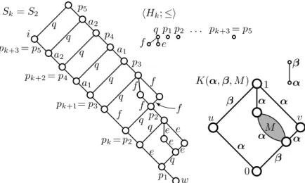
Figure 3. Sk fork= 2,hHk;≤i, andK(α,β, M); the ele- mentsa1, . . . , ak are defined after (3.2)
Figure 4. Elementary steps towards (5.3)
It is straightforward to check thatK(α,β) is colored (not only quasi- colored) by the two-element chain {α < β}, as indicated in Figure 1. Of course, we can rename the elements of this chain. For later reference, letM be a simple lattice, and letK(α,β, M) denote the colored lattice we obtain fromK(α,β) so that we replace its thick prime interval, see Figure 1, byM as indicated in Figure 3; all edges of M are colored byα. In Section 7, we will rely on the obvious fact that
whatever we do with K(α,β) in this section, we could do it with K(α,β, M1), K(α,β, M2), . . . , where M1,M2,. . . are finite simple lattices.
(5.2)
Let Sk be the lattice defined by Figure 3. Also, this figure defines an ordered set hHk;≤i. Let eγk: Prime(Sk) →Hk be given by the labeling; we claim that
γek: Prime(Sk)→ hHk;≤i is a coloring; see Figure 3. (5.3) Note that the colors, see (5.3), of the edges of the chain [w, i] of Sk are the same as the labels, see (2.4), of the edges of the corresponding filter of C∗. We obtain (5.3) by applying Lemma 4.3 repeatedly; the first three steps are given if Figure 4; the rest of the steps are straightforward. In Figure 4, going from left to right, we construct larger and larger quasi-colored (in fact, colored) lattices by Hall-Dilworth gluing. The colors are given by labeling and their ranges by small diagrams in which the elements are given by half-sized little circles. The action of gluing is indicated by “} ⇒”. Now that we have decomposed the task into elementary steps, we can conclude (5.3) easily.
Next, letγnat0 : Prime(L0)→J(Con(L0)) be the natural coloring ofL0, that is, for p ∈ Prime(L0), we have that γnat0 (p) = conL0(p). Using that ϕ0: Con(L0)→D0 is a lattice isomorphism, see after (3.5), we conclude that its restriction ψ0 := ϕ0eJ(Con(L0)) is an order isomorphism from J(Con(L0)) onto J(D0). Therefore, the composite map γ1 := ψ0 ◦ γnat0 is a coloring γ1: Prime(L0)→ hJ(D0);≤i. For later reference, note that
ψ0(conL0(p)) =ψ0(γnat0 (p)) = (ψ0◦γnat0 )(p) =γ1(p). (5.4) By 2.1(iiib),C∗is a filter ofL0, whereby the filter↑L0wis a chain. Hence, Lis the Hall–Dilworth gluing of L0 andSk; compare Figures 1 and 3. As a preparation to the next application of Lemma 4.3, we denote the ordered sets hJ(D0);≤iandhHk;≤ialso byhJ(D0);ν1iandhHk;ν2i, respectively. We let γ2 = eγk; see (5.3). Finally, L0 and Sk will also be denoted by L1 and L2, respectively. With these notations, letγbe the map defined in (4.4). On the set H :=J(D0)∪Hk, we define a quasiordering ν according to (4.5); note that the pairs ha1, a1i, . . . ,hak, aki required by (4.5) can be omitted. This means that
ν= quo ν1∪ν2∪ {hp, p1i,hp1, pi,hp, p2i,hp2, pi, . . . , hp, pk+3i,hpk+3, pi}
. (5.5)
We conclude from Lemma 4.3 that
γ: Prime(L)→ hH;νiis a quasi-coloring. (5.6) Letδ: hH;νi → hJ(D);≤ibe the map defined by
δ(x) =
(p, ifx∈ {p1, p2, . . . , pk+3},
x, otherwise. (5.7)
Observe that ifhx, yi ∈ν1∪ν2 orx, y∈ {p, p1, . . . , pk+3}, thenδ(x)≤δ(y).
Hence, the set generating ν in (5.5) is a subset of Ker(δ); see (4.2) and~ thereafter. This implies thatν ⊆Ker(δ) since~ Ker(δ) is a quasiordering. The~ inclusion just obtained means thatδis a homomorphism. In order to verify
the converse inclusion,Ker(δ)~ ⊆ν, assume that x6=y andhx, yi ∈Ker(δ),~ that is,δ(x)≤δ(y) inJ(D). There are four cases to consider.
First, assume thatx, y ∈ J(D0). Thenx =δ(x)≤ δ(y) = y in J(D).
ButJ(D0) is a subposet ofJ(D), wherebyhx, yi ∈ν1⊆ν, as required.
Second, assume that{x, y} ∩J(D0) =∅. Sincex, y∈ {p1, . . . , pk+3, q}, x6=y,{δ(x), δ(y)} ⊆ {p, q}, pkq, and δ(x)≤δ(y), we conclude thatxand y belong to {p1, . . . , pk+3}, whereby the required containment hx, yi ∈ν is clear by (5.5).
Third, assume thatx∈J(D0) buty /∈J(D0). Ify∈ {p1, . . . , pk+3}, then the requiredhx, yi ∈νfollows fromhx, pi ∈ν1⊆νandhp, yi ∈ν. Otherwise, y=q, andx=δ(x)≤δ(q) =qgives that hx, ei ∈ν1⊆ν orhx, fi ∈ν1⊆ν.
Sincehe, qi,hf, qi ∈ν2⊆ν, the requiredhx, yi ∈ν follows by transitivity.
Fourth, assume that x 6∈ J(D0) but y ∈ J(D0). Since δ(x) ∈ {p, q}
and δ(x) ≤ δ(y) = y ∈ J(D0), the only possibility is that δ(x) = p, x is in {p1, . . . , pk+3}, and y = p, whereby (5.5) yields the required hx, yi ∈ ν.
Therefore,Ker(δ)~ ⊆ν. Thus, it follows from (5.6) and Lemma 4.2 that the map
bγ=δ◦γ: Prime(L)→ hJ(D);≤i, defined byr7→δ(γ(r)), (5.8) is a coloring; this coloring is the same what the labeling in Figure 1 suggests.
By Lemma 4.1, the map µ: hJ(Con(L));≤i → hJ(D);≤i described in the lemma is an order isomorphism. By the well-known structure theorem of finite distributive lattices,µextends to a unique isomorphismϕ: Con(L)→D. We claim that
an element x of D belongs to ϕ(Princ(L)) if and only if there is a chainu0≺u1≺ · · · ≺un inLsuch thatx=γ([ub 0, u1])∨ · · · ∨bγ([un−1, un]).
(5.9) We are going to derive this fact only from the assumption thatbγis a coloring and ϕ is the isomorphism what bγ determines by Lemma 4.1; see between (5.8) and (5.9).
In order to prove (5.9), assume that there is such a chain. Then, applying Lemma 4.1 at the second equality below,
x=bγ([u0, u1])∨ · · · ∨γ([ub n−1, un])
=µ(con(u0, u1))∨ · · · ∨µ(con(un−1, un))
=ϕ(con(u0, u1))∨ · · · ∨ϕ(con(un−1, un))
=ϕ(con(u0, u1)∨ · · · ∨con(un−1, un)) =ϕ(con(u0, un)),
(5.10)
which implies that x ∈ ϕ(Princ(L)). Conversely, assume x ∈ ϕ(Princ(L)), that is, x= ϕ(con(a, b)) for some a≤ b ∈L. Let us pick a maximal chain a=u0≺u1≺ · · · ≺un=b in the interval [a, b], then (5.10) shows that xis of the required form. This proves the validity of (5.9).
We say that a (5.9)-chain u0≺u1≺ · · · ≺un producesxif the equality in (5.9) holds. In order to show that Q = ϕ(Princ(L)), we need to show that an element x∈D is produced by a (5.9)-chain iff x∈Q. It suffices to consider join-reducible elements and chains of length at least two, because
chains of length 1 produce join-irreducible elements that are necessarily in Qand, in addition, every join-irreducible x is produced by a (5.9)-chain of length 1 sincebγis surjective.
First, assume thatx∈Q\J0(D). Ifx∈Q\ ↓p, then xis of the form x=ai∨q, and we can clearly find a chain of length 2 inSk ⊆Lwithbγ-colors ai and q, and this is a (5.9)-chain that produces x. Otherwise, x ∈ Q0 = Q∩ ↓p. We obtain from (5.4) that the coloringγ1: Prime(L0)→ hJ(D0);≤i determines the order isomorphismψ0: J(Con(L0)→ hJ(D0);≤i in the same way as the coloring in Lemma 4.1 determinesµ. By the structure theorem of finite distributive lattices, ψ0 has exactly one extension to a Con(L0)→D0 isomorphism; this extension isϕ0 sinceψ0=ϕ0eJ(Con(L0)); see the paragraph above (5.4). Thus,
γ1 determines ϕ0 in the same way as bγ
determinesϕ; see between (5.8) and (5.9). (5.11) From (4.4), the paragraph preceding (5.4), and (5.6) we see that γ extends γ1. So, since δ defined in (5.7) acts identically on J(D0), bγ defined in (5.8) also extendsγ1. Combining this fact with (5.11), we obtain that
ϕandbγextendϕ0 andγ1, respectively. (5.12) By the choice ofϕ0: Con(L0) →D0, we have that x ∈Q0 =ϕ0(Princ(L0)).
Therefore, (5.9) applied to hD0, L0, ϕ0, γ1i rather than to hD0, L0, ϕ0,bγi, the sentence after (5.9), (5.11), and (5.12) imply that there exists a (5.9)-chain inD (in fact, even withinD0) that producesx.
Second, assume thatxis produced by a (5.9)-chainW of length at least 2. If W has a p-colored edge with respect to bγ, then ↑p ⊆ Q implies that x∈Q. Hence, with respect to bγ,
we can assume that no edge ofW is colored by p. (5.13) If W is a chain in L0, then applying (5.9) to hD0, L0, ϕ0, γ1i rather than to hD, L, ϕ,bγiand using (3.6) and (5.12), we obtain that the elementxbelongs to ϕ0(Princ(L0)) = Q0 ⊆ Q. If W had an edge both inside L0 and outside L0, that is, if ∅ 6= Prime(W)∩Prime(L0)6= Prime(W), thenW would have an edge [uj−1, uj] such that uj−1 ∈L0\C∗ but uj ∈C∗, since L is a Hall- Dilworth gluing ofL0andSk. In Figure 1, [uj−1, uj] is one of the dashed lines.
It would follow from Theorem 2.1(iiid) and (5.12) thatbγ([uj−1, uj]) = 1D0 = p, which would contradict (5.13). Thus,W cannot have an edge both inside L0 and outside L0. We are left with the case where W is a chain in Sk. In Sk, any two edges of W with distinct bγk-colors outside {p1, . . . , pk+3, q} are separated by an edge ofW whosebγk-color is in{p1, . . . , pk+3, q}; see Figure 3.
Formulating this withinL withbγ rather than γ2 =γbk, any two edges ofW with distinct bγ-colors not in{p, q} are separated by an edge of W whose bγ- color is in{p, q}; see Figure 1. Hence, the structure ofSk, see Figures 1 and 3, and (5.13) imply thatxis one of the elementse=e∨e,f =f∨f,e∨q=q, f ∨q =q, and ai∨q for i = 1, . . . k+ 3, and these elements belong to Q.
Hence,x∈Qfor everyW. Consequently,Q=ϕ(Princ(L)). This completes the proof of the (iii)⇒(i) part of Corollary 1.4.
6. A new approach to Gr¨ atzer’s Theorem 2.1
Part 2.1(i) is proved in Gr¨atzer [15]; we do not have anything to add. Part 2.1(ii) is an evident consequence of (the more general but technical) part 2.1(iii). This section is devoted to the proof of part 2.1(iii). Our approach includes a lot of ingredients from Gr¨atzer [15].
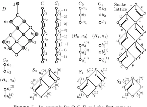
Proof of 2.1(iii). Assume that Q is a chain-representable subset of a finite distributive latticeD; see Figure 5, where Qconsists of the grey-filled ele- ments. The largest elements ofD will be denoted by111, it belongs to J(D) by our assumption. Let hC,lab, Di be aJ(D)-labeled chain representingQ.
We need to find a latticeLand an isomorphismϕ: Con(L)→D that satisfy the requirements of 2.1(iii).
Figure 5. An example for Q ⊆ D and the first steps to- wards its representation
The ordering ofJ(D) will often be denoted byκ0. Take a list hC0;κ00i, . . . ,hCt−1;κ0t−1i
of chains inJ(D); hereκ0idenotes the restriction ofκ0toCi, fori < t. Assume that this list of chains is taken so thatJ(D)\ {1D}=S
i<tCi, and quo (J(D)× {111})∪[
i<t
κ0i
=κ0, that is, (J(D)× {111})∨_
i<t
κ0i=κ0 (6.1)
in Quo(J(D)). Note that although we can always take the list of all chains {a, b}witha≺J(D)b, we often get a much smaller latticeLby selecting fewer chains. For example, for the latticeD given in Figure 5, we can let t = 3, C0={a1< a2< a3},C1={b1< b2< b3}, andC2={b2< a3}. For each of the chainsCi={x1< x2<· · ·< xmi}=hCi;κ0iisuch thatmi>1, let
Hi ={x(i)1 < x(i)2 <· · ·< x(i)mi}=hHi;κii (6.2) be an alter ego of Ci; see Figure 5 again. Each of the hHi;κii, for i < t, determines asnake lattice, which is obtained by gluing copies ofK(α,β) so that there is a coloringσifrom the set of prime intervals of the snake lattice ontohHi;κii. For example, ifhHi;κiihad been{p < q < r < s < u < v < x}, then the snake lattice would have been the one given on the top right of Figure 5. For our example,this exemplary snake lattice is not needed; what we need for our D are the Si and the colorings σi: Prime(Si) → hHi;κii, indicated by labels in the figure, for i < t. (By space considerations, not all edges are labeled.) The purpose of the alter egos is to make our chains Hi
pairwise disjoint. If mi =|Ci| = 1, then Si is the two-element lattice and the coloringσi is the unique map from the singleton Prime(Si) tohHi;κii:=
h{xi1};κii, whereκi is the only ordering on the singleton setHi.
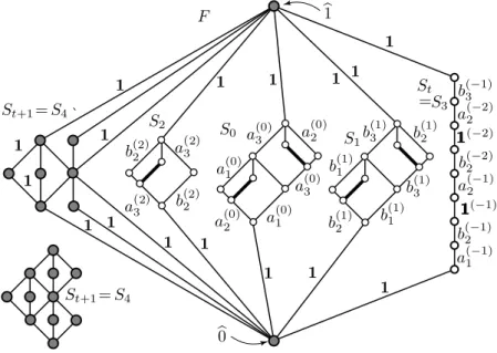
Figure 6. The frame lattice F for the example given in Figure 5 andSt+4=S4
Next, we turnhC,lab, Di, see Figure 5, to a colored latticeStas follows.
Before its formal definition, note that in our example, St =S3 is given in Figure 5. As a lattice,St :=C. Forx∈J(D), let h(x) =|{p∈Prime(C) :
lab(p) =x}|; note thath(x)≥1 since lab is a surjective map. Let Ht:= [
x∈J(D)
{x(−1), . . . , x(−h(x))} and κt:={hy, yi:y∈Ht}; (6.3) thenhHt;κtiis an antichain, which is not given in the figure. Define the map
σt: Prime(St) → Ht by the rule p 7→ x(−i) iff lab(p) = x and, counting from below,p is thei-th edge ofClabeled byx. (6.4) Less formally, we make the labels ofSt=C pairwise distinct by using neg- ative superscripts; see Figure 5. (The superscripts are negative, because the positive ones have been used for another purpose in (6.2).) The new labels with negative superscripts form an antichain Ht, and the new labeling σt
becomes a coloring.
The colored lattices Si, i ≤ t, with their colorings σi: Prime(Si) → hHi;κii will be referred to under the common name branches. So the i-th branch is a snake lattice or the two-element lattice for i < t, and it is the colored chainStwith the coloring given in (6.4) fori=t.
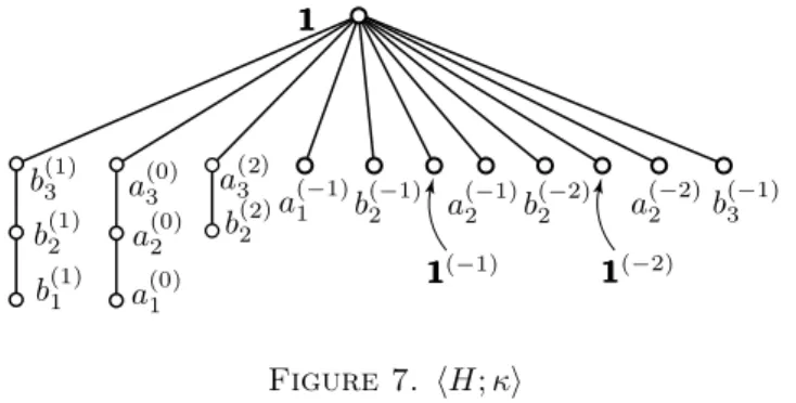
Figure 7. hH;κi
Next, lethHt+1;κt+1ibe the one-element ordered setHt+1={111}, and letSt+1be an arbitrary simple lattice with|St+1| ≥3. (6.5) In Figure 6,St+1consists of the elements given by a bit larger and grey-filled circles. We have chosen this simple lattice because it is easy to draw. The zero and the unit ofSt+1 will be denoted by b0 andb1, respectively. Note the notational difference: whileb0 andb1 are inSt+1and they will be in the lattice Lwe are going to construct,111and000are inDandH, and they will correspond to congruences of L. The unique map Prime(St+1) → hHt+1;κt+1i will be denoted byσt+1; it is a coloring. All the lattices and ordered sets mentioned so far in this section are assumed to be pairwise disjoint. LetF be the lattice we obtain fromSt+1 by inserting all theSifori≤tas intervals such that for everyi, j∈ {0, . . . , t},xi∈Si,xj∈Sj andyt+1∈St+1\ {b0,b1}, we have that xi∨yt+1=b1,xi∧yt+1=b0, and ifi6=j, then we also have thatxi∨xj=b1 and xi∧xj = b0; see Figure 6, which gives F for our example of Q ⊆ D given in Figure 5. Following Gr¨atzer [15], we callF theframe or theframe lattice associated with Q⊆D, but note that it depends also on the list of
chains and the choice ofSt+1. The simplicity ofSt+1 guarantees thatF is a {b0,b1}-separating lattice. In order to see this, letx∈L\ {b0,b1}. If x∈St+1, then con(b0, x) = con(x,b1) = 1Con(F)by the simplicity ofF. Ifx /∈St+1, then xhas a complementy inSt+1, and con(b0, x) = con(x,b1) = 1Con(F)since the same holds fory. Let
H := [
i<t+2
Hi, κ:= (H× {111})∪ [
i<t+2
κi, and define
σ(p) =
(σi(p), ifp∈Prime(S0)∪ · · · ∪Prime(St), 111, otherwise.
(6.6)
Clearly, (6.6) above defines a quasiordered set hH;κi together with a map σ: Prime(F) → hH;κi. In case of our example, σ and hH;κi are given by Figures 6 and 7, respectively. Clearly, κ is always an ordering. Using that F is{b0,b1}-separating and arguing similarly to Gr¨atzer [15], it is easy to see that σ is a coloring. Fori < t+ 1, the subsets Hi are called the legs ofH. Fori < t, thei-th legHi is a chain, and it is an antichain fori=t.
Figure 8. Equalizing the colorsg andh
Each element ofJ(D)\{111}has at least one alter ego inH, but generally it has many alter egos; they differ only in their superscripts. The alter egos of an element x ∈ J(D) with positive superscripts belong to distinct legs.
Note at this point that forx∈J(D) and−1≥ −s≥ −h(x), see (6.3),x(−s) is also called an alter ego ofx. Note also that111also has alter egos, usually many alter egos, inSt. It is neither necessary, nor forbidden that111has alter
egos inS0∪ · · · ∪St−1. Next, let
ε={hg0, h0i,hh0, g0i,hg1, h1i,hh1, g1i, . . . ,
hgm−1, hm−1i,hhm−1, gm−1i} ⊆H2 (6.7) be a symmetric relation such that the equivalence relation equ(ε) generated byεis the least equivalence onH that collapses every element with all of its alter egos. Every “original color”x(that is, everyx∈J(D)) has an alter ego in Ht and also in some other leg Hi0 such that i0 < t. Quasi-colorings are surjective by definition. Thus, sinceσextendsσifori < t+ 1 by (6.6) andx has only one alter ego inHi0 fori0< t, we can assume that
for every hg`, h`i ∈ ε, there are distinct branches Si and Sj such thatSi contains an edgepi withσ(pi) =σi(pi) =g` and Sj contains an edgepj withσ(pj) =σj(pj) =h`.
(6.8) Note that the smaller the ε is, the smaller the lattice L will be. Since ε is symmetric,
the equivalence equ(ε) generated byεis quo(ε). (6.9) Hence, letting η:= quo(κ∪ε), we have that equ(ε)⊆η. (6.10) We claim that for everyx, y∈J(D),
x≤y in J(D) iff there exist alter egos x0 and y0 of
xandy, respectively, such thatx0≤ηy0. (6.11) In order to see this, assume first thatx≤y inJ(D), that is,x≤κ0 y. We can assume thaty6=111, because otherwisehx, yi ∈κby (6.6), wherebyhx, yi ∈η;
see (6.10). By (6.1), there is a sequencex=z0, z1, . . . , zn =y inJ(D)\ {111}
such that hzj, zj+1i ∈S
i<tκ0i for allj < n. So for every j < n, we can pick anij ∈ {0, . . . , t−1} such thathzj, zj+1i ∈ κ0ij, that is, hzj(ij), z(ij+1j)i ∈ κij. Hence,
hzj(ij), z(ij+1j)i ∈κij (6.6)
⊆ κ
(6.10)
⊆ η hold for allj < n. (6.12) For allj < n−1, the elements zj+1(ij) and z(ij+1j+1) are alter egos of the same zj+1, whereby (6.9) and (6.10) give thathzj+1(ij), zj+1(ij+1)i ∈η. This fact, (6.12), and the transitivity of η imply that hx0, y0i := hz0(i0), zn(in−1)i ∈ η. That is, there exist alter egosx0 and y0 ofxandy, respectively, such thatx0 ≤η y0.
Second, to prove the converse implication, assume thatx0 ≤η y0for alter egos ofxandy, respectively. Again, we can assume thaty6=111. It suffices to deal with the particular casex0 ≤κi y0, because the casehx0, y0i ∈εcauses no problem and the general case follows from the particular one by (6.6), (6.10), and transitivity. Butx0 ≤κi y0 means thatxandy belong to the same chain Ci and x ≤y in this chain. Hence,x ≤y in J(D), as required. Therefore, (6.11) holds.
Next, we explain where the rest of the proof and that of the construction go. Let δ:hH;ηi → hJ(D);≤i, defined by δ(x) = y iff x is an alter ego of y. Since Ker(δ) =~ η by (6.11), we conclude thatδ is a homomorphism; see
between (4.2) and Lemma 4.2. Assume that we can find a lattice L and a mapγ such that
γ: Prime(L)→ hH;ηiis a coloring. (6.13) Then, using that hJ(D);≤i is an ordered set, not just a quasiordered one, Lemma 4.2 will imply that the map bγ:=δ◦γ is a coloringbγ: Prime(L)→ hJ(D);≤i. In the next step, it will turn out by Lemma 4.1 that
µ: hJ(Con(L));≤i → hJ(D);≤i, defined by
con(p)7→γ(p), in an order isomorphism.b (6.14) Furthermore, (5.9) will be valid forLby the same reason as in Section 5;
see the sentence following (5.9). At present, by the choice of St and the definition ofF,
the elements x ∈ D that are of the form described in (5.9),
with F instead ofL, are exactly the elements ofQ. (6.15) For`∈ {0,1, . . . , m}, see (6.7), let
ε`:={hgj, hji:j < `} ∪ {hhj, gji:j < `} and η`:= quo(κ∪ε`). (6.16) By (6.10), η0 = κ, εm = ε, and ηm = η. By induction, we are going to find{0,1}-separating lattices L0=F,L1, . . . , Lmand quasi-colorings γ0 = σ: Prime(L0) → hH;η0i and, for ` ∈ {1, . . . , m}, γ`: Prime(L`) → hH;η`i such that “ the elements described in (5.9) remain the same”, that is, for every`in {1, . . . , m} andx∈L`,
x=bγ`([u0, u1])∨ · · · ∨γb`([un−1, un]) for some elements u0≺u1≺ · · · ≺un ofL` iff the same equality holds for some elementsu0≺u1≺ · · · ≺un ofC.
(6.17) Roughly speaking, (6.17) says that (6.15) remains valid. Note that γ` will extend γ`−1, for ` ∈ {1, . . . , m}. Since γ0 = σ and L0 := F satisfy the requirements, including (6.17), it is sufficient to deal with the transition from L`−1 toL`, for 1≤`≤m.
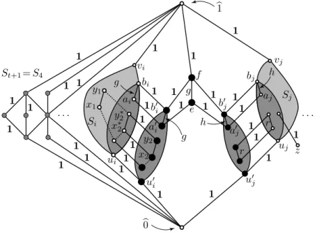
So we assume thatγ`−1: Prime(L`−1)→ hH;η`−1isatisfies the require- ments formulated in the induction hypothesis above, including (6.17). In or- der to ease the notation in Figure 8, we denotehg`−1, h`−1ibyhg, hi. Then, as it is clear from (6.16),η`= quo(η`−1∪{hg, hi}∪{hh, gi}). Hence, we shall add an “equalizing flag”W toL`−1such that this flag forces that the congruence generated by ag-colored edge be equal to the congruence generated by anh- colored edge. The term “flag” and its usage are taken from Gr¨atzer [15]. Apart from terminological differences, the argument about our flag is basically the same as that in Gr¨atzer [15]. (Note that our interval [ui, bi] in Figure 8 need not be a chain; it is always a chain in Gr¨atzer [15], but this fact is not ex- ploited there.) By (6.8), there are distinct i, j ∈ {0,1, . . . , t} such that we can choose theg-colored edge and theh-colored edge mentioned above from branches Si and Sj, respectively; see Figure 8. Since the role of g and his symmetric, we can assume thati < j.
In Figure 8, the flag is [u0i, b0i]∪ {e, f} ∪[u0j, b0j]. So the large black-filled elements belong to the flag. Note that not all elements of the flag are indicated
![Figure 1. D with two coatoms, K(α, β), and L that we construct conjunction of Cz´ edli [8, Proposition 1.6] and Gr¨ atzer [15], here we deal only with the case where 1 = 1 D is join-reducible](https://thumb-eu.123doks.com/thumbv2/9dokorg/1318003.106206/5.659.89.568.87.428/figure-coatoms-construct-conjunction-edli-proposition-atzer-reducible.webp)