A CONVEX COMBINATORIAL PROPERTY OF COMPACT SETS IN THE PLANE AND ITS ROOTS IN LATTICE THEORY
GÁBOR CZÉDLI AND ÁRPÁD KURUSA
Dedicated to George A. Grätzer
on the occasion of the fifty-fifth anniversary of the Grätzer–Schmidt Theorem and the fortieth anniversary of his monograph “General Lattice Theory"
Abstract. K. Adaricheva and M. Bolat have recently proved that if U0
and U1 are circles in a triangle with vertices A0, A1, A2, then there exist j ∈ {0,1,2} and k ∈ {0,1} such that U1−k is included in the convex hull of Uk∪({A0, A1, A2} \ {Aj}). One could say disks instead of circles. Here we prove the existence of such a j and kfor the more general case where U0and U1are compact sets in the plane such that U1 is obtained from U0
by a positive homothety or by a translation. Also, we give a short survey to show how lattice theoretical antecedents, including a series of papers on planar semimodular lattices by G. Grätzer and E. Knapp, lead to our result.
1. Aim and outline
Our goal. Apart from a survey of historical nature, which the reader can skip over if he is interested only in the main result, this paper belongs to elementary combinatorial geometry. The motivation and the excuse that this paper is sub- mitted to CGASA are the following. The first author has recently written a short biographical paper [16] to celebrate professor George A. Grätzer, and also an inter- view [17] with him; at the time of this writing, both have already appeared online in CGASA. Although [16] mentions that G. Grätzer’s purely lattice theoretical results have lead to results in geometry, no detail on the transition from lattice theory to geometry is given there. This paper, besides presenting a recent result in geome- try, exemplifies how such a purely lattice theoretical target as studying congruence lattices of finite lattices can lead, surprisingly, to some progress in geometry.
The real plane and the usual convex hull operator on it will be denoted by R2 and ConvR2. In order to formulate our result, we need the following two kinds of planar transformations, that is,R2→R2 maps. GivenP ∈R2 and0< λ∈R, the positive homothetywith (homothetic) center P and ratioλis defined by
χP,λ: R2→R2 byX7→(1−λ)P+λX =P+λ(X−P). (1.1) h12,17i Date:CET 03:20, July 10, 2018.
2010Mathematics Subject Classification. Primary 52C99, secondary 52A01, 06C10.
Key words and phrases. Congruence lattice, planar semimodular lattice, convex hull, compact set, circle, combinatorial geometry, abstract convex geometry, anti-exchange property.
1
The more general concept of homotheties where λ can also be negative is not needed in the present paper. For a givenP ∈R2, the mapR2 →R2, defined by X7→P+X, is atranslation. Our main goal is to prove the following theorem.
Theorem 1.1. Let A0, A1, A2 ∈R2 be points of the plane R2. Also, let U0 ⊂R2 and U1⊂R2be compact sets such that at least one of the following three conditions holds:
(a) U1 is a positive homothetic image of U0, that is, U1=χP,λ(U0)for some P ∈R2 and0< λ∈R;
(b) U1 is obtained from U0 by a translation;
(c) at least one of U0 and U1 is a singleton.
With these assumptions,
if U0∪ U1⊆ConvR2({A0, A1, A2}), then there exist subscripts j∈ {0,1,2} andk∈ {0,1} such that
U1−k ⊆ConvR2 Uk∪({A0, A1, A2} \ {Aj}) .
(1.2) h2,8,9,11,13,18,20,23i
Since at least one of the conditions 1.1(a), 1.1(b), and 1.1(c) holds for any two circles, the following result of Adaricheva and Bolat becomes an immediate consequence of Theorem1.1.
Corollary 1.2(Adaricheva and Bolat [2, Theorem 3.1]). Let U0and U1becircles in the planeR2. Then(1.2)holds for all A0, A1, A2∈R2.
Four comments are appropriate here. First, according to another terminology, positive homotheties (in our sense) and translations generate the group of positive homothety-translations, and one might think of using homothety-translations in Theorem 1.1. It will be pointed out in Lemma 3.9 that we would not obtain a new result in this way, because a homothety-translation is always a homothety or a translation. Since the rest of the paper focuses mainly on homotheties in our sense, we use disjunction rather than the hyphened form “homothety-translation”.
Second, it is easy to see that (1.2) does not hold for two arbitrary compact sets, so the disjunction of (a), (b), and (c) cannot be omitted from Theorem 1.1; see also Czédli [14] for related information. Third, Example 4.1 of Czédli [15] rules out the possibility of generalizing Theorem 1.1 for higher dimensions. Fourth, one may ask whether stipulating the compactness of U0 and U1 is essential in Theorem1.1. Clearly, “compact” could be replaced by “(topologically) closed”, since a non-compact closed set cannot be a subset of the triangle ConvR2({A0, A1, A2}), but this trivial rewording would not be a valuable improvement. The situation
A0:=h6,0i, A1:=h−3,3√
3i, A2:=h−3,−3√ 3i,
U0:={hx, yi:x2+y2<1} ∪ {hx, yi:x2+y2= 1andxis rational}, U1:={hx, yi:x2+y2<1} ∪ {hx, yi:x2+y2= 1andxis irrational},
exemplifies that Theorem1.1would fail without requiring the compactness of U0
and U1.
Prerequisites and outline. No special prerequisites are required; practically, every mathematician with usual M.Sc. background can understand the proof of Theorem 1.1. On the other hand, Section 2 is of historical nature and can be interesting mainly for specialists.
The rest of the paper is structured as follows. In Section2, starting from lattice theoretical results including Grätzer and Knapp [41, 42, 43, 44, 45], we survey how lattice theoretical results lead to the present paper. Also, we say a few words on some similar results that belong to combinatorial geometry. Section 3 proves Theorem1.1only for the particular case where the convex closures of the compact sets U0and U1 are “edge-free” (to be defined later). Section4reduces the general case to the edge-free case and completes the proof of Theorem1.1.
2. From George Grätzer’s lattice theoretical papers to geometry Congruence lattices of finite lattices are well known to form George Grätzer’s favorite research topic, in which he has proved many nice and deep results; see, for example, the last section in the biographical paper [16] by the first author.
At first sight, it is not so easy to imagine interesting links between this topic and geometry. The aim of this section is to present such a link by explaining how some of Grätzer’spurely lattice theoretical results have lead to the present paper and other papers ingeometry. Instead of over-packing this section with too many definitions and statements, we are going to focus onlinks connecting results and publications. This explains that, in this section, some definitions are given only after discussing the links related to them. Although a part of this exposition is based on the experience of the first author, the link between lattice theory and the geometrical topic of the present paper is hopefully more than just a personal feeling.
2.1. Planar semimodular lattices and their congruences. On November 28, 2006, Grätzer and his student, Edward Knapp submitted their first paper, [41], to Acta Sci. Math. (Szeged) on planar semimodular lattices. A latticeL =hL;∨,∧i issemimodular if, for everya∈L, the mapL→L, defined byx7→a∨x, preserves the “covers or equal” relation ; as usual, a b stands for |{x ∈ L : a ≤ x ≤ b}| ∈ {1,2}. A lattice is planar if it is finite and has a Hasse diagram that is also a planar graph. Their first paper, [41], were soon followed by Grätzer and Knapp [42,43,44,45]. After giving a structural description of planar semimodular lattices, they proved nice results on the congruence lattices of these lattices in [42], [44], and [45].
The lattice Con(L)of all congruence relations ofLis thecongruence latticeofL, and it is known to be a distributive algebraic lattice by an old result of Funayama and Nakayama [35]. It is a milestone in the history of lattice theory that not every
distributive latticeDcan be represented in the form of Con(L); this famous result is due to Wehrung [59]. However,
every finite distributive latticeDcan be represented, up
to isomorphism, as Con(L)whereLis a finite lattice. (2.1) h4i
This result is due to Dilworth, see [6], but it was not published until Grätzer and Schmidt [47]. There are several ways of generalizing (2.1); the first four of the following targets are due to G. Grätzer or to G. Grätzer and E. T. Schmidt.
(T1) Find anL with nice properties in addition to Con(L)∼=D, (T2) find anL of size being as small as possible,
(T3) represent two or even more finite distributive lattices and certain isotone maps among them simultaneously,
(T4) represent a finite ordered set (also known as a poset) as the ordered set of principal congruences of a finite lattice, and
(T5) combine some of the targets above.
There are dozens of results and papers addressing these targets. The monograph Grätzer [36] surveyed the results of this kind available before 2006. Ten years later, the new edition [40] became much more extensive, and the progress has not yet finished. The series of papers by Grätzer and Knapp fits well into the targets listed above. Indeed, [44] fits (T1) by providing arectangular latticeLwhile, fitting both (T1) and (T2), [45] minimizes the size of this rectangularL. A rectangular lattice is a planar semimodular lattice with a pair hu, vi 6= h0,1i of double irreducible elements such that u∧v = 0 and u∨v = 1; these lattices have nice rectangle- shaped planar diagrams.
Next, in their 2010 paper, Grätzer and Nation [46] proved a stronger form of the classical Jordan–Hölder theorem for groups from the nineteenth century. Here we formulate their result only for groups, but note that both [46] and [25], to be mentioned soon, formulated the results for semimodular lattices. For subnormal subgroupsA / B and C / D of a given group G, the quotient B/A is said to be subnormally down-and-up projectivetoD/Cif there are subnormal subgroupsE /F such thatAF =B, A∩F =E,CF =D, andC∩F =E. Grätzer and Nation’s result for finite groups says that whenever {1} = X0 / X1/· · ·/ Xn = G and {1}=Y0/ Y1/· · ·/ Ym=Gare composition series of a groupG, thenn=mand
there exists a permutation π:{1, . . . , n} → {1, . . . , n} such that Xi/Xi−1is subnormally down-and-up projective to Yπ(i)/Yπ(i)−1 for alli∈ {1, . . . , n}.
(2.2) h4,7i
(The original Jordan–Hölder theorem states only that the quotient groupsXi/Xi−1 and Yπ(i)/Yπ(i)−1 are isomorphic, because they are in the transitive closure of subnormal down-and-up projectivity.) Not much later, Czédli and Schmidt [25]
added thatπ in (2.2) is uniquely determined. The proof in [25] is based on slim planar semimodular lattices; this concept was introduced in Gätzer and Knapp
[41]: a planar semimodular lattice isslim if M3, the five-element nondistributive modular lattice, cannot be embedded into it in a cover-preserving way.
Next, (T1)–(T5) and the applicability of slim semimodular lattices for groups motivated further results on the structure of slim semimodular lattices, including Czédli [8], Czédli and Grätzer [19], Czédli, Ozsvárt and Udvari [24], and Czédli and Schmidt [26] and [27]. Some results on the congruences and congruence lattices of these lattices, including Czédli [9], [12], [13], Czédli and Makay [23], Grätzer [38], [39], and Grätzer and Schmidt [48] and [49] have also been proved. Neither of these two lists is complete; see the book sections Czédli and Grätzer [20] and Grätzer [37]
and the monograph Grätzer [40] for additional information and references.
2.2. Convex geometries as combinatorial structures. It was an anonymous referee of Czédli, Ozsvárt and Udvari [24] who pointed out that slim semimodu- lar lattices can be viewed as convex geometries of convex dimension at most 2;
see Proposition2.1 and the paragraph following it in the present paper. As the first consequence of this remark, Adaricheva and Czédli [3] and Czédli [10] gave a lattice theoretical new proof of the “coordinatizability” of convex geometries by permutations; the original combinatorial result is due to Edelman and Jamison [31].
As we know from Monjardet [55], convex geometries are so important that they had been discovered or rediscovered in many equivalent forms even by 1985 not only as combinatorial structures but also as lattices. This explains that the terminology is far from being unique. Here we go after the terminology used in Czédli [10] even when much older results are cited. If the reader is interested in further information on convex geometries, he may turn to [10] for a limited survey or to Adaricheva and Nation [5] for a more extensive treatise. To keep the size limited, we do not mention antimatroids and meet-distributivity; see the survey part of Czédli [10] for references on them.
In order to give a combinatorial definition, the power set of a given finite set E will be denoted by Pow(E) :={X :X ⊆E}. If a mapΦ :Pow(E)→Pow(E) satisfies the rules X ⊆Φ(X)⊆Φ(Y) = Φ(Φ(Y))for all X ⊆Y ⊆E, then Φis a closure operator over the set E. A pair hE; Φi is aconvex geometry ifE is a nonempty set,Φis a closure operator overE, Φ(∅) =∅, and, for all p, q∈E and X= Φ(X)∈Pow(E), theanti-exchange property
(p6=q, p /∈X, q /∈X, p∈Φ(X∪ {q}) )⇒q /∈Φ(X∪ {p}) (2.3) holds. For example, ifE is a finite set of points of R2, then we obtain a convex geometryhE; Φiby letting
Φ :Pow(E)→Pow(E) defined by Φ(X) :=E∩ConvR2(X). (2.4) h7i
The dual of a lattice K = hK;∨,∧i is denoted by Kdual := hK;∧,∨i. For x∈ K, let x∗ := W{y : x ≺y}. Let M3 denote the five-element modular non- distributive lattice. By a join-distributive lattice we mean a semimodular lattice of finite length that does not include M3 a sublattice. (This concept should not
be confused with join-semidistributivity.) Equivalently, a semimodular lattice K of finite length isjoin-distributive if the interval [x, x∗] is a distributive lattice for allx∈ K \ {1}; this is the definition that explains the current terminology. From the literature, Czédli [10, Proposition 2.1] collects eight equivalent definitions of join-distributivity; the oldest one of them is due to Dilworth [29].
Given a convex geometry hE; Φi, the set {X ∈Pow(E) :X = Φ(X)} ofclosed sets forms a lattice with respect to set inclusion⊆. The dual of this lattice will be denoted byLlat(hE; Φi). As usual, a set X ∈Pow(E) is called open if E\X is closed. With this terminology, Llat(hE; Φi)can be considered as the lattice of open subsets ofE with respect to set inclusion⊆.
For a finite lattice K, the set J(K) of (non-zero) join-irreducible elements is defined as {x ∈ K : there is exactly oney ∈ Kwithy ≺ x}. Next, for a finite latticeL, we define a closure operator
ΦLdual:Pow(J(Ldual))→Pow(J(Ldual)) by ΦLdual(X) :=n
y∈J(Ldual) :y≤Ldual
_
Ldual
Xo
, and we let Gconv(L) :=hJ(Ldual); ΦLduali.
Of course, the inequality above is equivalent toy≥V
X in LandJ(Ldual)equals the set of meet-irreducible elements ofL. The following proposition, cited as the combination of Proposition 7.3 and Lemma 7.4 in [10], is due to Adaricheva, Gor- bunov, and Tumanov [4] and Edelman [30].
Proposition 2.1. Let hE; Φi andL be a convex geometry and a join-distributive lattice, respectively. Then Llat(hE; Φi) is a join-distributive lattice, Gconv(L) is a convex geometry, and, in addition, we have thatGconv(Llat(hE; Φi))∼=hE; Φi and Llat(Gconv(L))∼=L.
This proposition allows us to say that convex geometries and join-distributive lattices capture basically the same concept. Based on Proposition2.1and the the- ory of planar semimodular lattices summarized in Czédli and Grätzer [20], we can say that a convex geometryhE; Φiis ofconvex dimensionat most 2 ifLlat(hE; Φi) is a slim semimodular lattice.
2.3. From lattices to convex geometries by means of trajectories. In order to describe the first step from Grätzer and Knapp [41,42,43,44,45] and Grätzer and Nation [46] towards geometry, we need to define trajectories. Ifa≺bin a finite latticeK, then [a, b]is called a prime interval of K. The set of prime intervals of Kwill be denoted by PrIntv(K). Two prime intervals,[a0, b0],[a1, b1]∈PrIntv(K), are consecutive if ai = a1−i∧bi and b1−i = a1−i∨bi hold for some i ∈ {0,1}.
The reflexive-transitive closure of consecutiveness is an equivalence relation on PrIntv(K), and its classes are called thetrajectories ofK.
Trajectories were introduced in Czédli and Schmidt [25], and they played the key role in proving the uniqueness ofπin (2.2). Soon afterwards, trajectories were intensively used when dealing with congruence lattices of slim planar semimodular lattices, because forx≺yanda≺bis such a lattice, one can describe with the help of trajectories whether the least congruence con(a, b)collapsing ha, bicontains (in other words, collapses)hx, yi. Later, similarly to trajectories, a beautiful descrip- tion of the containmenthx, yi ∈con(a, b)was described by Grätzer’s Swing Lemma;
see Grätzer [38], and see Czédli, Grätzer, and Lakser [21] and Czédli and Makay [23]
for a generalization and for alternative approaches. Note that Lemma 2.36 in Freese, Ježek, and Nation [34, page 41], which is due to Jónsson and Nation [51]
originally, offers an alternative way to describe whetherhx, yi ∈con(a, b).
For distinct prime intervals[a0, b0],[a1, b1]∈PrIntv(K), we say that[a0, b0]and [a1, b1] arecomparable if either b0 ≤a1, or b1 ≤a0. It was proved in Adaricheva and Czédli [3] that
(a finite semimodular lattice L is join-distributive if and only if no two distinct comparable prime intervals of L belong to the same trajectory.
(2.5) h7i
Combining (2.5) with Proposition2.1, we obtain a new description of convex ge- ometries.
2.4. Representing convex geometries. Using the usual convex hull operator ConvRn together with auxiliary points in a tricky way, Kashiwabara, Nakamura, and Okamoto [52] gave a representation theorem for convex geometries in 2005. The example described in (2.4) is simpler, but it is not appropriate to representevery convex geometry because of a very simple reason: ifhE; Φiis a convex geometry of the form described in (2.4), thenJ(Llat(hE; Φi))is an antichain, which is not so for every convex geometry. Hence, Czédli [11] introduced the following construction.
LetE be a finite set of circles in the planeR2, and define a convex geometryhE; Φi whereΦ :Pow(E)→Pow(E)is defined by
Φ(X) :=n
C∈E:C⊆ConvR2
[
D∈X
Do
. (2.6) h7,8i
It is easy to see that we obtain a convex geometry in this way. Note, however, that (2.6) does not yield a convex geometry in general if, say, E is a set of triangles rather than a set of circles. After translating the problem to lattice theory with the help of Proposition2.1 and using the toolkit developed for slim semimodular lattices in the papers mentioned in Subsection2.1, Czédli [11] proved that
every convex geometry of convex dimension at most2can rep-
resented by circles in the sense of (2.6). (2.7) In fact, [11] proves a bit more. While [11] is mainly a lattice theoretical paper, it was soon followed by two results with proofs that are geometrical. First, Richter and Rogers [56] represented every convex geometry analogously to (2.6) but using
polygons instead of circles. Second, Czédli and Kincses [22] replaced polygons with objects taken from an appropriate family of so-called “almost circles”. However, it was not known at that time whether circles would do instead of “almost circles".
2.5. Some results of geometrical nature. The problem whether every con- vex geometry can be represented by circles in the sense of (2.6) was solved in negative by Adaricheva and Bolat [2]. The main step in their argument is the proof of [2, Theorem 3.1]; see Corollary 1.2 here. In fact, they proved that (1.2), with self-explanatory syntactical refinements, holds even for arbitrary threecircles A0, A1, A2 and two additional circles, U0,U1. This is such an obstacle that does not allow to represent every convex geometry by circles. Even more is true; later, Kincses [53] found an Erdős–Szekeres type obstruction for representing convex ge- ometries byellipses. Similarly to ellipses, he could exclude many other shapes. On the positive side, Kincses [53] proved that every convex geometry can be repre- sented byellipsoids in Rn for some n∈ N+ :={1,2,3, . . .} in the sense of (2.6) with ConvRn instead of ConvR2. However, it is not known whethern-dimensional balls could do instead of ellipsoids.
An earlier attempt to generalize Adaricheva and Bolat [2, Theorem 3.1], see Corollary1.2here, did not use homotheties and resulted in a new characterization of disks. Namely, for a convex compact set U0⊆R2, Czédli [14] proved that
U0 is a disk if and only if for every isometric copy U1 of U0 and
for any pointsA0, A1, A2∈R2, (1.2) holds. (2.8) h8i
The condition on U1above means that there exists a distance-preserving geometric transformationϕ:R2→R2 such that U1=ϕ(U0).
There are quite many known characterizations of circles and disks; we mention only one of them below. We say that U0 and U1 are Fejes-Tóth crossing if none of the sets U0\ U1andU1\ U0 is path-connected. It was proved in Fejes-Tóth [33]
that
a convex compact set U0 ⊆R2 is a disk if and only if there is no isometric copy U1 of U0 such that U0 and U1 are Fejes-Tóth crossing.
(2.9) h8i
Motivated by the proof of (2.8), a more restrictive concept of crossing was intro- duced in Czédli [18]; it is based on properties of common supporting lines but we will not define it here. Replacing Fejes-Tóth crossing with “[18]-crossing”, (2.9) turns into a stronger statement.
Finally, to conclude our mini-survey from George Grätzer’s congruence lattices to geometry via a sequence of closely connected consecutive results, we note that Paul Erdős and E. G. Straus [32] extended (2.9) to an analogous characterization of balls in higher dimensions, but the “[18]-crossing” seems to work only in the planeR2.
3. Proofs for the edge-free case
As usual in lattice theory, U ⊂ V means the conjunction of U ⊆ V and U 6=V.
IfV is a compact subset of R2, then we often write V ⊂ R2 sinceV 6= R2 holds automatically. For compact sets U,V ⊆R2,
ConvR2 U ∪ V) =ConvR2 ConvR2(U)∪ V .
Hence, the inclusion in the third line of (1.2) is equivalent to the inclusion ConvR2(U1−k)⊆ConvR2 ConvR2(Uk)∪({A0, A1, A2} \ {Aj})
.
Also, if U is compact, then so is ConvR2(U); see, for example, the first sentence of the introduction in Hüsseinov [50]. Thus, it suffices to prove our theorem only for convex compact subsets ofR2. Therefore, in the rest of the paper,
we will always assume that U, U0, and U1
are compact andconvex, (3.1) h9,23i
even if this is not repeated all the time.
The advantage of assumption (3.1) lies in the fact that the properties of planar convex compact sets are well understood. For example, ifU ⊂R2is such a set, then the boundary∂U of U is known to be a simple closed continuous rectifiable curve;
see Latecki, Rosenfeld, and Silverman [54, Thm. 32] and Topogonov [58, page 15].
Since the reader need not be a geometer, we note that all what we need to know about planar convex sets are surveyed in a short section of the open access paper Czédli and Stachó [28]. Some facts about these sets, however, are summarized in the next subsection for the reader’s convenience.
3.1. Supporting lines and a comparison with the case of circles. Let Cunit denote theunit circle {hx, yi:x2+y2= 1}; (3.2) its elements are called directions. In the rest of the paper, we often assume that the lines`in our considerations aredirected lines; their directions are denoted by dir(`)∈ Cunitand by arrows in our figures. A directed line`determines twoclosed halfplanes; their intersection is`. A subset ofR2 is on the left of ` if each of its points belongs to the left closed halfplane. Points in the left halfplane of ` but not on ` are strictly on the left of `; pointsstrictly on the right of ` are defined analogously. We always assume that
na supporting line of a set U is directed, and it is
directed so that U is on its left. (3.3) h10i
Since every compact convex set in the plane is well known to be the intersection of the left halfplanes of its supporting lines, we have that
if a pointP ∈ R2 does not belong to a compact convex set U, then U has a directed supporting line ` such that P is strictly on the right of`.
(3.4) h22i
If` is a supporting line of a compact convex set U, then the points of U ∩` are called support points. If ` is the only directed supporting line through a support point P ∈ U ∩`, then ` is a tangent line and P is a tangent point. Otherwise, we say thatP is a vertex of U. The properties of directed supporting lines are summarized in the open access papers Czédli [14] and Czédli and Stachó [28], or in the more advanced treatise Bonnesen and Fenchel [7]. In particular, by apointed supporting lineof U we mean a pairhP, `isuch that`is a directed supporting line of U with support pointP. In general, U may have pointed supporting lineshP1, `i andhP2, `iwith the same line component but distinct support points P16=P2.
In Czédli [15], which is devoted only to circles, there is a relatively short proof of Adaricheva and Bolat [2, Theorem 3.1], cited as Corollary 1.2here. Most ideas of [15] are used in the present paper, but these ideas need substantial changes in order to overcome the following three difficulties: as opposed to circles, a compact convex set need not have a center with nice geometric properties, its boundary need not have a tangent line at each of its points, and the boundary can include straight line segments of positive lengths. In this section, we disregard the latter difficulty by calling a compact convex set U edge-free if no line segment of positive length is a subset of∂U. Equivalently, a compact convex set U ⊂R2 is said to beedge-free if`∩ U is a singleton (still equivalently, if`∩∂U is a singleton) for every supporting line`of U. Note that every singleton subset ofR2is an edge-free compact convex set. Let us emphasize that an edge-free set isnonempty by definition. In order to shed even more light on the concept just introduced, we formulate and prove an easy lemma.
Lemma 3.1. A nonempty compact convex set U is edge-free if and only if`∩∂U consists of at most two points for every line`.
Proof. We can assume that U is not a singleton since otherwise the statement is trivial.
First, assume that U is not edge-free, and pick a supporting line ` of U with two distinct points, P1, P2 ∈ `∩∂U. LetP3 = (P1+P2)/2; it belongs to U by convexity. SinceP3 lies on a supporting line, it is not in the interior of U. Hence, P1, P2, P3∈`∩∂U, which shows that`∩∂U consists of more than two points; this implies the “if” part of the lemma.
Second, assume that U is edge-free and`is a directed line in the plane; we need to show that`∩∂U consists of at most two points. Suppose the contrary, and let P1,P2, andP3be three distinct points of`, in this order, such that they all belong also to∂U. Pick a supporting line`2of U throughP2. Since U is edge-free,`2∩∂U is a singleton, whereby none ofP1andP3lies on`2. Therefore, sinceP2is between P1 andP3, we have thatP1 ∈ U and P3 ∈ U are strictly on different sides of `2;
contradicting (3.3).
Our target in the present section is to prove the following lemma.
Lemma 3.2(Main Lemma). If the pointsA0, A1, A2∈R2and the convexcompact sets U0,U1⊂R2 from Theorem 1.1satisfy at least one of the conditions (a),(b), and(c)given in the theorem and, in addition,
(d) U0 and U1 are edge-free, then implication(1.2)holds.
The proof of this lemma needs some preparation and auxiliary lemmas. In the rest of this section, we always assume that U0 and U1 areedge-free.
3.2. Comets. In this paper, the Euclidean distance((Px−Qx)2+ (Py−Qy)2)1/2 of P, Q ∈ R2 is denoted by dist(P, Q). For nonempty compact sets U,V ⊂ R2, dist(U,V) = inf{dist(P, Q) : P ∈ U, Q ∈ V}= min{dist(P, Q) :P ∈ U, Q∈ V}.
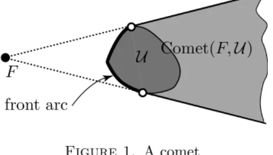
For an edge-free compact convex set U with more than one elements and a point F∈R2\ U, we define thecometComet(F,U)withfocus F andnucleus U so that
Figure 1. A comet
Comet(F,U)is the grey-filled area in Figure1. (3.5) More precisely, if we consider F as a source of light, then Comet(F,U) is the topological closure of the set of points that are shadowed by the nucleus U. Note that U, which is dark-grey in the figure, is a subset of Comet(F,U)and we have that dist({F},Comet(F,U))>0. As opposed to U, Comet(F,U)is never compact.
Since U is compact, convex, and not a singleton, there are exactly two supporting lines of U throughF, and they are supporting lines of Comet(F,U)as well. Since U is edge-free, these two lines aretangent lines of U and also of Comet(F,U). Each of these tangent lines has a unique tangent point on∂U. The arc of ∂U between these points that is closer toF is thefront arc of the comet; see the thick curve in Figure1. Note that the boundary of Comet(F,U)is the union of the front arc and two half-lines, so comets are never edge-free.
3.3. Externally perspective compact convex sets. For topologically closed convex setsV1,V2⊆R2, we will say that
V1isloosely included inV2, in notation, V1
loose
⊂ V2, (3.6)
if every point ofV1 is an internal point of V2. The interior of a compact convex set U will be denoted by Int(U); note that Int(U) =U \∂U. Clearly, ifV1⊂R2is compact,V2⊆R2 is closed, andP ∈Int(V1), then
( V1
loose
⊂ V2 implies that there is a δ > 0 such that χP,1+ε(V1)loose⊂ V2for all positiveε≤δ,
(3.7) h20i
becauseR2\Int(V2)is closed and its distance fromV1 is positive.
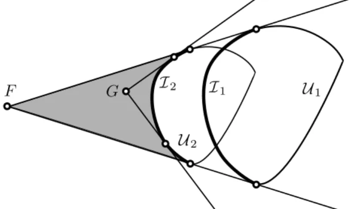
Next, for compact convex sets U1,U2 ⊂R2, each of them with more than one element, we say that U1 and U2 are externally perspective if U2 =χP,λ(U1)for some (in fact, unique)0< λ∈R\ {1} andP ∈R2\ConvR2(U1∪ U2); see (1.1).
Equivalently, U1 and U2areexternally perspective if U2=χP,λ(U1)withP /∈ U1
and0< λ6= 1. Hence, by interchanging the subscripts if necessary, we will often assume that0< λ <1if U2=χP,λ(U1)is externally perspective to U1.
Figure 2. Illustration for Lemma3.3 The following lemma is obvious by Figure2.
Lemma 3.3. Let U1and U2=χF,λ(U1)be externally perspective compact convex subsets of the plane such that0< λ <1. IfGis an internal point of the grey-filled area surrounded by the common tangent lines of U1and U2throughF and the front arcI2 of Comet(F,U2), thenComet(F,U1)is loosely included inComet(G,U2).
In the rest of the paper, to ease the notation,
4A0,A1,A2 will stand for ConvR2({A0, A1, A2}). (3.8) h17,20i
Next, as a “loose counterpart” of the 2-Carousel Rule defined in Adaricheva [1], we formulate the following lemma.
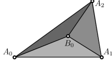
Lemma 3.4. Let A0, A1, and A2 be non-collinear points in the plane. If B0
andB1 are distinct internal points of 4A0,A1,A2, then there existj ∈ {0,1,2} and
k∈ {0,1} such that
{B1−k}loose⊂ ConvR2 {Bk} ∪({A0, A1, A2} \ {Aj}) .
Figure 3. Illustration for the proof of Lemma3.4
Proof. If B1 is in the interior of one of the three little triangles that are colored with different shades of grey in Figure3, then we can letk:= 0. Otherwise,B1is an internal point of one of the line segments[A0, B0], [A1, B0], and[A2, B0], and we can letk := 1. In both cases, it is clear that we can choose an appropriate
j∈ {0,1,2}.
Lemma 3.5. Condition 1.1(c), even without assuming 3.2(d), implies(1.2), that is, the conclusion of Lemma 3.2.
Proof. Since U0 and U1 play symmetric roles, we can assume that U0 ={B0} is a singleton. We can assume also thatB0∈Int(4A0,A1,A2), because otherwise the statement is trivial. If there exists a pointB1 ∈ U1 and a subscript j ∈ {0,1,2}
such that
B0∈ConvR2 {B1} ∪({A0, A1, A2} \ {Aj})
, (3.9) h13i
then (1.2) holds with k = 1 and this j. So, we assume that (3.9) fails for all B1∈ U1and allj∈ {0,1,2}. Then, by Lemma3.4ifB1below is in Int(4A0,A1,A2) or trivially ifB1∈∂4A0,A1,A2,
for each B1 ∈ U1, there is a smallest j =j(B1)∈ {0,1,2} such that B1∈ConvR2 {B0} ∪({A0, A1, A2} \ {Aj(B1)})
. (3.10) h13i
Ifj=j(B1)does not depend onB1∈ U1, then (3.10) gives the satisfaction of (1.2) withk= 0and thisj. For the sake of contradiction, suppose that j(B1)depends onB1 ∈ U1. By (3.10), this means that there are pointsB01 and B100 in U1 that belong to distinct little triangles (colored by different shades of grey) in Figure3.
By convexity,[B10, B100]⊆ U1. Hence, U1has a pointB1 that belongs to one of the line segments[A0, B0], [A1, B0], and[A2, B0]. ThisB1 shows the validity of (3.9) for somej, which contradicts our assumption that (3.9) fails for allj. Thus,j(B1) does not depend onB1∈ U1, completing the proof.
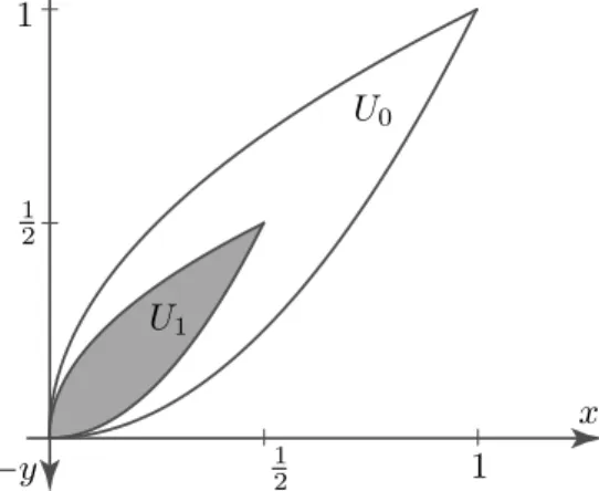
3.4. Internally tangent edge-free compact convex sets. We say that U0and U1subject to1.1(a) or1.1(b) areinternally tangent if they have a common pointed supporting line. For example, as it is shown in Figure4, if
Figure 4. Two internally tangent edge-free compact convex sets U0:={hx, yi: 0≤x≤1, x2≤y≤1−(x−1)2} and
U1:=χh0,0i,1/2(U0), (3.11) h14i
then U0 and U1 are internally tangent edge-free compact convex sets. Let O = h0,0i. Denoting the abscissa axis with the usual orientationh1,0i ∈ Cunit and the ordinate axis with the unusual reverse orientationh0,−1i ∈ Cunit by x and −y, respectively, bothhO, xiandhO,−yiare common pointed supporting lines of U0
and U1. This shows that condition 1.1(a) together with3.2(d) do not imply the uniqueness of the common supporting lines through a point of ∂U0∩∂U1 if U0
and U1 are internally tangent. In case of (3.11) and similar cases, these pointed supporting lines have the same support point and U0 and U1 are tangent to each other in some sense. The aim of this subsection is to prove the following lemma.
Lemma 3.6. If U0 and U1 are non-singleton, internally tangent, edge-free com- pact convex subsets of R2, then the following two assertions hold.
(i) If U1 = χP,λ(U0) for some 0 < λ ∈ R and P ∈ R2, as in 1.1(a), then either U1=U0 andλ= 1, or λ6= 1 and∂U0∩∂U1={P}. Furthermore, ifλ >1 then U1⊇ U0 while0< λ <1 implies that U1⊆ U0.
(ii) If U1 is obtained from U0by a translation as in 1.1(b), then U1=U0 and the translation in question is the identity map.
Note that this lemma fails without assuming that U0and U1 are edge-free. To exemplify this, let U0 be the rectangle{hx, yi:−2≤x≤2and0≤y≤2}. Then U1:=χh4,2i,1/2(U0)and U1:={hx+ 1, yi:hx, yi ∈ U0}would witness the failure of3.6(i) and that of3.6(ii), respectively.
Proof. LethP∗, `∗ibe a common pointed supporting line of U0 and U1.
First, assume that U1 = χP,λ(U0) as in (i). We can assume that U0 6= U1
since otherwise the lemma is trivial. So we know that0 < λ6= 1. SincehP∗, `∗i is a pointed supporting line of U0, so is hP0, `0i:= hχP,λ(P∗),χP,λ(`∗)iof U1 = χP,λ(U0). We have that dir(`0) =dir(`∗); note that this is one of the reasons that λ >0 is always assumed in this paper. It is well known from the folklore that for eachα∈ Cunit and every compact convex set U,
U has exactly one directed supporting line of directionα; (3.12) h22i
see Bonnesen and Fenchel [7], Yaglom and Boltyanskiˇı [60, page 8], or Czédli and Stachó [28]. Hence,`0and`∗are the same supporting lines of U1. Since U1is edge- free,`∗=`0has only one support point, whenceP∗=P0. SoP∗=P0=χP,λ(P∗).
Sinceλ 6= 1, the homothetyχP,λ has only one fixed point, whereby P∗ =P, as required. Next, let Q be an arbitrary element of ∂U0∩∂U1. For the sake of contradiction, suppose that Q6=P. Sinceλ6= 1, thecollinear points P, Q, and Q0 := χP,λ(Q) are pairwise distinct. Since the χP,λ-image of a boundary point is a boundary point, these three collinear points belong to∂U1. This contradicts Lemma3.1and settles the first sentence of (i).
Since χP,1/λ is the inverse ofχP,λ, it suffices to prove the second sentence of (i) only for λ > 1, because then the case 0 < λ < 1 will follow by replacing hU0,U1, λi by hU1,U0,1/λi. So, let X be an arbitrary point of U0. Using that X ∈ConvR2({P,χP,λ(X)}), P =P∗ =P0 ∈ U1, and χP,λ(X)∈χP,λ(U0) =U1, the convexity of U1 implies thatX ∈ U1, as required. This completes the proof of part (i).
The argument for (ii) is similar. Let ϕdenote the translation such that U1 = ϕ(U0). Let hP0, `0i := hϕ(P∗), ϕ(`∗)i. As in the previous paragraph, we obtain thathP0, `0iand hP∗, `∗iare both supporting lines of U1. Since dir(`0) =dir(`∗), we have that`0 =`∗. Thus, using that U1 is edge-free, we obtain that P0 =P∗. SoP0=ϕ(P∗)is a fixed point of the translation ϕ. Hence,ϕis the identity map, and we conclude thatU1=ϕ(U0) =U0, as required.
3.5. Technical lemmas. We compose maps from right to left, so note the rule (ϕ◦ψ)(x) =ϕ ψ(x)
. The first technical lemma we need is the following.
Lemma 3.7. Let ϕ:R2→R2 be a homothety χP,λ or a translation, letP0∈R2 be a point, and letP1=ϕ(P0). Then for every ξ∈R\ {0},
ϕ◦χP
0,ξ=χP
1,ξ◦ϕ or, equivalently, χP
1,ξ=ϕ◦χP
0,ξ◦ϕ−1. Proof. Since ϕ◦χP
0,ξ◦ϕ−1 is clearly a homothety of ratio ξ that fixes P1, this homothety isχP
1,ξ, as required.
The next technical lemma will also be needed. It follows by straightforward com- putation with the help of computer algebra; an appropriate worksheet for Maple
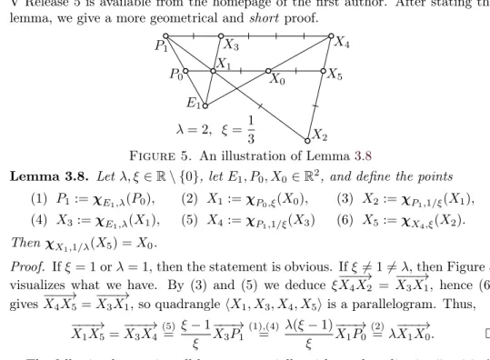
V Release 5 is available from the homepage of the first author. After stating the lemma, we give a more geometrical andshort proof.
Figure 5. An illustration of Lemma 3.8
Lemma 3.8. Letλ, ξ∈R\ {0}, letE1, P0, X0∈R2, and define the points (1) P1:=χE
1,λ(P0), (2) X1:=χP
0,ξ(X0), (3) X2:=χP
1,1/ξ(X1), (4) X3:=χE1,λ(X1), (5) X4:=χP1,1/ξ(X3) (6) X5:=χX4,ξ(X2).
ThenχX1,1/λ(X5) =X0.
Proof. Ifξ= 1orλ= 1, then the statement is obvious. Ifξ6= 16=λ, then Figure5 visualizes what we have. By (3) and (5) we deduce ξ−−−→
X4X2 = −−−→
X3X1, hence (6) gives−−−→
X4X5=−−−→
X3X1, so quadrangle hX1, X3, X4, X5iis a parallelogram. Thus,
−−−→X1X5=−−−→
X3X4(5)= ξ−1 ξ
−−−→X3P1(1),(4)= λ(ξ−1) ξ
−−−→X1P0(2)= λ−−−→
X1X0. The following lemma is well known, especially without the adjective “positive”.
However, there are other variants and the corresponding terminology is not unique in the literature; for example, Schneider [57, page xii] includes translations in the concept of positive homotheties. The terminological ambiguity in the literature justifies that we formulate this lemma and give its trivial proof.
Lemma 3.9. LetGbe the collection of all positive homotheties and all translations of the plane. ThenGis a group with respect to composition.
Proof. It suffices to show that if ϕ1 and ϕ2 belongs to G, then so does ϕ :=
ϕ1◦ϕ2. Sinceϕ1andϕ2are similarity transformations that preserve the directions of directed lines, the same holds forϕ. This implies thatϕ∈G.
3.6. The lion’s share of the proof. First, we prove the following lemma.
Lemma 3.10. Assume that U0 is an edge-free compact convex subset of R2, ϕ:R2 →R2 is a positive homothety or a translation, U1=ϕ(U0),P0∈Int(U0), P1 =ϕ(P0), ξ ∈ (0,1) = [0,1]\ {0,1}, U0(ξ) = χP0,ξ(U0), U1(ξ) = χP1,ξ(U1), and U0(ξ) and U1(ξ) are internally tangent. Then at least one of the following two assertions hold:
(i) U0⊆ U1 and U0(ξ)⊆ U1(ξ), or (ii) U1⊆ U0 and U1(ξ)⊆ U0(ξ).
Proof. We can assume thatϕis not the identity map, since otherwise the statement trivially holds. Computing by Lemma3.7, we obtain that
U1(ξ) =χP1,ξ ϕ(U0)
= (χP1,ξ◦ϕ◦χP0,1/ξ) U0(ξ)
Lem.3.7
= (ϕ◦χP
0,ξ◦χP
0,1/ξ) U0(ξ)
=ϕ U0(ξ)
, (3.13) h17i
which shows that Lemma 3.6 is applicable to the triplet hU0(ξ),U1(ξ), ϕi. Let hE1, `i be a common pointed supporting line of U0(ξ) and U1(ξ). Since ϕ is not the identity map, Lemma 3.6 gives that ϕ = χE
1,λ for some λ > 0. The systems hU0,U1, λ, ϕ = χE1,λi and hU1,U0,1/λ, ϕ−1 = χE1,1/λi play symmetric roles, whence we can assume thatλ≥1. We obtain by Lemma 3.6that
U0(ξ)⊆ U1(ξ). (3.14) h17i
In order to prove the inclusion U0 ⊆ U1, let X0 ∈ U0. Since ϕ = χE1,λ, we have thatP1=χE
1,λ(P0). Consider the pointsX1, . . . , X5defined in Lemma3.8.
By the definition of U0(ξ), we have that X1 ∈ U0(ξ), whereby (3.14) yields that X1∈ U1(ξ). Thus, sinceχP1,1/ξis the inverse ofχP1,ξ, the definition of U1(ξ)leads toX2∈ U1. SinceX1∈ U0(ξ), we obtain by equation (4) of Lemma3.8,χE1,λ=ϕ, and (3.13) that X3 ∈ U1(ξ). This gives that X4 ∈ U1. Since X2, X4 ∈ U1 and 0< ξ <1, the convexity of U1 implies thatX5∈ U1. Using thatX1∈ U1(ξ)⊆ U1
and that 0 <1/λ ≤1, the convexity of U1 gives that χX1,1/λ(X5) ∈ U1. Thus, X0∈ U1 by Lemma3.8, proving that U0⊆ U1, as required.
Now, armed with the auxiliary statements proved so far, we are in the position to prove the (Main) Lemma3.2.
Proof of Lemma3.2. Lemma 3.5 allows us to assume that none of U0 and U1
is a singleton. For the sake of contradiction, suppose that the lemma fails. Let U0,U1, A0, A1, andA2witness this failure. We can assume thatA0,A1, andA2is the counterclockwise list of the vertices of triangle4A0,A1,A2; see (3.8). If 1.1(a) holds, thenϕ:R2→R2 will denote the transformationχP,λmentioned in 1.1(a).
Similarly, if 1.1(b) holds, thenϕ:R2 → R2 stands for a translation according to 1.1(b). In both cases, U1 = ϕ(U0). Fix an internal point P0 of U0, and let P1:=ϕ(P0). Fori∈ {0,1}and every real numberξ∈[0,1], let
Ui(ξ) :=χPi,ξ(Ui). (3.15) h17,18,19,20i
Note thatχP
i,ξis a positive homothety only forξ >0but (1.1) is meaningful also forλ= 0. In particular, Ui(0) :=χPi,0(Ui) makes sense and it is understood as {Pi}. Forξ= 0, we trivially have that U1(ξ) =ϕ U0(ξ)
. So letξ >0. Lemma3.7 and (3.15) yield that
U1(ξ) =χP1,ξ(U1)
= (ϕ◦χP0,ξ) ϕ−1(U1)
=ϕ χP0,ξ(U0)
=ϕ(U0(ξ)). (3.16) h19i
Thus,
U1(ξ) =ϕ U0(ξ)
, for allξ∈[0,1]andi∈ {0,1}. (3.17) Since Ui(ξ)⊆ Ui(1) =Ui⊆ 4A0,A1,A2, we have also that Ui(ξ)⊆ 4A0,A1,A2.
LetH be the set of allη∈[0,1]such that (1.2) holds for U0(η)and U1(η)with somejandk. Since0∈Hby Lemma3.5, or even by Lemma3.4,H6=∅. Hence,H has a supremum, which we denote byξ. It follows from Lemma3.4and continuity thatξ >0. A standard compactness argument shows thatξ∈H, that is,ξis the maximal element ofH. Since a more involved, similar, but still standard argument will be given after (4.5), we do not give the details of this compactness argument here; note that the omitted details, modulo insignificant changes, are given in the extended version, arXiv:1610.02540, of Czédli [15]. Taking our indirect assumption andξ= max(H)into account, we have that
0< ξ := max(H)<1. (3.18) h21i
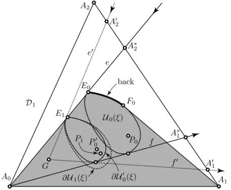
Sinceξ∈H, we can assume that the indices are chosen so that, as Figure6shows, U1(ξ)is included in the grey-filled “curved-backed trapezoid”
Trp(ξ) :=ConvR2({A0, A1} ∪ U0(ξ)). (3.19) In Figure6, the “back” of this trapezoid is the thick curve connectingE0and F0. If U1(ξ) was included in the interior of Trp(ξ), then there would be a (small) positiveεsuch that U1(ξ+ε)⊆Trp(ξ)⊆Trp(ξ+ε)andξ+εwould belong toH, contradicting the fact thatξ is the largest element ofH. Hence, U1(ξ)⊆Trp(ξ), but the intersection∂U1(ξ)∩∂Trp(ξ)has at least one point. So we can pick a point E1 ∈∂U1(ξ)∩∂Trp(ξ). Since U1(ξ) loose⊂ U1(1) =U1 ⊆ 4A0,A1,A2, we have that E1 ∈/ ∂4A0,A1,A2. Since the “left leg”, that is, the straight line segment [A0, E0], and the “right leg” [A1, F0] of Trp(ξ) play symmetric roles, it suffices to consider only the following two cases: eitherE1 belongs to the “back” of Trp(ξ), including its endpointsE0andF0, orE1 belongs to the “left leg” [A0, E0], excludingE0.
First, assume thatE1belongs to the “back” of Trp(ξ). Then, clearly,E1belongs to ∂U0(ξ). Since Trp(ξ) is a compact convex set, it has a directed supporting line ` through E1. Since U0(ξ) ⊆Trp(ξ) and U1(ξ) ⊆Trp(ξ), both U0(ξ) and U1(ξ) are on the left of `. Using that E1 is in U0(ξ)∩ U1(ξ), it follows that hE1, `i is a common pointed supporting line of U0(ξ) and U1(ξ). Hence, U0(ξ) and U1(ξ) are internally tangent. Furthermore, it follows from Lemma 3.9 and (3.15) that U1(ξ)is obtained from U0(ξ)by a translation or a positive homothety.
Therefore, Lemma 3.10yields that U0 ⊆ U1 or U1 ⊆ U2. This trivially implies (1.2), contradicting the initial assumption of the proof. Thus, the first case where E1belongs to the back of Trp(ξ)has been excluded.
Second, assume that E1 belongs to the “left leg” [A0, E0] as illustrated in Fig- ure6. Since U1(ξ)loose⊂ U1⊆ 4A0,A1,A2implies thatE1∈/ ∂4A0,A1,A2, we have that E16=A0. We can assume thatE1 6=E0 since the opposite case has already been
Figure 6. Illustration for the proof of Lemma3.2
settled. Hence, lettingν :=dist(A0, E1)/dist(A0, E0), we have that0< ν <1. Let
U00:=χA0,ν(U0), P00:=χA0,ν(P0), (3.20) h19,20i
ϕ0 :=ϕ◦χA0,1/ν, and U00(ξ) :=χP0
0,ξ(U00). (3.21) h19,20i
The position of U00(ξ)in Figure6is justified by χA0,ν(U0(ξ)) (3.15)= (χA0,ν◦χP0,ξ)(U0)
Lem.3.7
= (χP0
0,ξ◦χA0,ν)(U0) (3.20)= χP0
0,ξ(U00) (3.21)= U00(ξ).
(3.22) h20i
SinceχA0,1/ν is the inverse ofχA0,ν, (3.20) and (3.21) yield that
P1=ϕ0(P00) and U1=ϕ0(U00). (3.23) h19,20i
Computing by Lemma3.7as in (3.16), we obtain that U1(ξ) (3.15)= χP1,ξ(U1) (3.23)= (χP1,ξ◦ϕ0)(U00)
Lem.3.7
= (ϕ0◦χP0
0,ξ)(U00) (3.21)= ϕ0 χP0
0,ξ(U00)
=ϕ0(U00(ξ)).
(3.24) h20i
According to Figure 6, the directed line through the “left leg” of Trp(ξ) will be denoted by e; clearly, E0, E1, A0 ∈ e. Since χA0,ν(E0) = E1, χA0,ν(e) = e, and