INTERSECT?
G ´ABOR CZ ´EDLI, L ´ASZL ´O OZSV ´ART, AND BAL ´AZS UDVARI
Abstract. LetH~ andK~ be finite composition series of lengthhin a groupG.
The intersections of their members form a lattice CSL(H , ~~ K) under set inclu- sion. Our main result determines the numberN(h) of (isomorphism classes) of these lattices recursively. We also show that this number is asymptotically h!/2. If the members ofH~ andK~ are considered constants, then there are exactlyh! such lattices.
Based on recent results of Cz´edli and Schmidt, first we reduce the problem to lattice theory, concluding that the duals of the lattices CSL(H , ~~ K) are exactly the so-called slim semimodular lattices, which can be described by permutations. Hence the results onh! andh!/2 follow by simple combinatorial considerations. The combinatorial argument proving the main result is based on Cz´edli’s earlier description of indecomposable slim semimodular lattices by matrices.
1. Introduction
The well-known concept of a composition series in a group goes back to ´Evariste Galois (1831), see Rotman [25, Thm. 5.9]. The Jordan-H¨older theorem, stating that any two composition series of a finite group have the same length, was also proved in the nineteenth century; see Jordan [21] and H¨older [20]. A stronger statement is obtained from the Schreier Refinement Theorem, see [25, Theorem 5.11]: if a group has a finite composition series, then any two of its composition series have the same length. Let
(1.1)
H~ : G=H0. H1.· · ·. Hh={1}, K~ : G=K0. K1.· · ·. Kh={1}
be composition series of a groupG. Here Hi−1. Hi denotes that Hi is a normal subgroup ofHi−1; the sequenceH~ is acomposition seriesifHiis a maximal normal proper subgroup ofHi−1, fori= 1, . . . , h. Denote the set
Hi∩Kj :i, j∈ {0, . . . , h}
by CSLh(H, ~~ K). The notation comes from “Composition Series Lattice”. Under containment, CSLh(H, ~~ K) is an ordered set. Sometimes we write CSL(H, ~~ K) for CSLh(H, ~~ K). Since CSLh(H, ~~ K) has a largest element and is closed with respect to
Date: May 14, 2011; last revision August 24, 2012.
1991Mathematics Subject Classification. Primary: 05A99; Secondary: 06C10, 05A05, 05E15, 20A99.
Key words and phrases. Composition series, group, Jordan-H¨older theorem, counting lattices, counting matrices, semimodularity, slim lattice, planar lattice, semimodular lattice.
This research was supported by the NFSR of Hungary (OTKA), grant numbers K77432 and K83219, and by T ´AMOP-4.2.1/B-09/1/KONV-2010-0005.
1
intersection, CSLh(H, ~~ K) is a finite lattice. The join ofX, Y ∈CSLh(H, ~~ K) is the intersection of{Z :X ⊆Z, Y ⊆Z andZ ∈CSLh(H, ~~ K)}. Let N(h) denote the number of isomorphism classes of all lattices CSLh(H, ~~ K) formed from composition series with lengthh. In other words,N(h) counts the number of lattices of the form CSLh(H, ~~ K); isomorphic lattices are counted only once.
If we view all the Hi and Kj as constants, then CSLh(H, ~~ K) becomes a mul- tipointed lattice, which we denote by CS¨Lh(H, ~~ K). If H~0 andK~0 are composition series of length hin a group G0, then the multipointed lattices CS¨Lh(H, ~~ K) and CS¨Lh(H~0, ~K0) are isomorphic if there is a lattice isomorphismϕ: CSLh(H, ~~ K)→ CSLh(H~0, ~K0) such thatϕ(Hi) =Hi0andϕ(Ki) =Ki0, fori= 0, . . . , h. The number of (isomorphism classes of) multipointed lattices CS¨Lh(H, ~~ K) of length h will be denoted by ¨N(h).
Our main goal is to determine N(h) and ¨N(h). Proposition 3.1 gives a sim- ple explicit formula for ¨N(h), and Proposition 7.1 gives a satisfactory asymptotic formula for N(h). Theorem 5.3, our main result, yields only a recursive way to compute N(h). Due to the fact that we count specific lattices, even this recursion is far more efficient than the best known way to compute all finite lattices of a given sizes; see Heitzig and Reinhold [19] fors≤18, and the references therein.
We will also consider the abstract class of lattices CSLh(H, ~~ K). This abstract class has recently been characterized by Cz´edli and Schmidt [11]. To make our approach self-contained and to give a sharper result, we give a direct proof of this characterization; see Proposition 2.3. Also, we prove a join-embedding result, Proposition 2.6, for the multipointed versions of these lattices.
Outline. Sections 2, 3, and 4 are lattice-theoretic, while Sections 5, 6, and 7 are combinatorial. Section 2 deals with the abstract class of lattices CSLh(H, ~~ K).
Section 3 proves Proposition 3.1, which asserts that ¨N(h) = h! (hfactorial). By recalling and supplementing the main result of Cz´edli [5], Section 4 translates the problem of determining N(h) to a purely combinatorial problem on certain 0,1- matrices. Sections 5 formulates the most difficult result in this paper, Theorem 5.3, which is a recursive formula for the exact value ofN(h). This section lists some concrete values ofN(h), computed by Maple and Mathematica. The main result is proved in Section 6. Finally, Section 7 proves thatN(h) is asymptotic toh!/2.
2. Composition series and slim semimodular lattices
2.1. Basic concepts and notation. The study of semimodular lattices is an im- portant branch of lattice theory; see Stern [28], Gr¨atzer [14] and [15], Nation [23], and Cz´edli and Schmidt [7] for surveys. Recall that a latticeL is (upper) semi- modular if a ≺ b implies a∨c b∨c, for all a, b, c∈ L. Similarly,L is lower semimodular or dually semimodular if it satisfies the dual property: abimplies a∧cb∧c, fora, b, c∈L. Note that CSL(H, ~~ K) will turn out to be lower semi- modular but generally is not semimodular. However, it suffices to count their dual lattices, which are semimodular. Therefore, since all the lattice-theoretic results that we reference were formulated for semimodular lattices, it is reasonable to work with semimodular lattices rather than lower semimodular ones.
Except for the lattice SubG of all subgroups of G (see below), all lattices in this paper are assumed to be of finite length, and mostly they are finite. Following
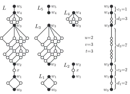
Gr¨atzer and Knapp [16], a finite lattice L is slim if there are no three pairwise incomparable join-irreducible elements inL. A diagram of an ordered set isplanar if its edges can be incident only at their endpoints. By Cz´edli and Schmidt [8, Lemma 2.2], every slim lattice isplanar, that is, it has a planar diagram. Hence slim semimodular lattices are easy to work with. In particular, a visual understanding is provided by Cz´edli and Schmidt [9], which clearly implies thatLin Figure 1 is a slim semimodular lattice.
Slim semimodular lattices have recently proved to be useful in strengthening a classical group theoretical result, namely, the Jordan-H¨older theorem. G. Gr¨atzer and Nation [18] proved that given two composition series of a group, as in (1.1), there is a matching between their quotients such that the corresponding quotients are isomorphic for a very specific reason: they are related by the composite of a down-perspectivity with an up-perspectivity. In Cz´edli and Schmidt [8], this matching is shown to be unique. Moreover, Cz´edli and Schmidt [11] have just proved that this matching determines the lattice CSL(H, ~~ K). The main role in [8]
and [11] is played by slim semimodular lattices. These lattices are also useful in lattice theory, see Cz´edli [6] and Cz´edli and Schmidt [10] for the latest results.
The relation “subnormal subgroup” is the transitive closure of “normal sub- group”. LetGbe a group with a finite composition series of lengthh. Its subnormal subgroups form a sublattice SnSubG= (SnSubG;⊆) of the lattice SubGof all sub- groups, by a classical result of Wielandt [29]; see also Schmidt [26, Theorem 1.1.5]
and the remark after its proof, or see Stern [28, p. 302]. It is not hard to see that SnSubGis dually semimodular, that is, lower semimodular; see [26, Theorem 2.1.8], or the proof of [28, Theorem 8.3.3], or the proof of Nation [23, Theorem 9.8].
Hence, forH~ andK~ defined in(1.1), CSLh(H, ~~ K) is also lower semimodular by the dual of Cz´edli and Schmidt [8, Lemma 2.4]. Note that the dual of [8, Lemma 2.4]
also asserts that CSLh(H, ~~ K) is acover-preservingmeet-subsemilattice of SnSubG, that is, ifX, Y ∈CSLh(H, ~~ K) andX≺Y in CSLh(H, ~~ K), thenX≺Y in SnSubG.
In general, CSLh(H, ~~ K) is distinct from SnSubG. This follows easily from (the abelian case of) the description of all finite groups with planar subgroup lattices, given by Schmidt [27], and the fact that CSLh(H, ~~ K) is always a planar lattice by Cz´edli and Schmidt [8, the dual of Lemma 2.2]. Furthermore, as witnessed by the 8-element elementary 2-group (Z2; +)3, CSLh(H, ~~ K) is not even a sublattice of SnSubGin general.
The set of non-zero join-irreducible elements and that of non-unit meet-irreducible elements of a finite latticeLwill be denoted by JiLand MiL, respectively. Let
H~ ∪K~ ={Hi: 0≤i≤h} ∪ {Ki: 0≤i≤h}.
Since Mi CSLh(H, ~~ K)
is obviously a subset ofH~ ∪K, the set Mi CSL~ h(H, ~~ K) contains no three-element antichain. Hence
(2.1) CSL(H, ~~ K) is a dually slim, dually semimodular lattice.
As usual,N denotes{1,2,3, . . .}, and N0 stands forN∪ {0}. The isomorphism class of a latticeL, that is, the class{L0:L0 ∼=L}, is denoted byI(L). IfK(y) is a class of lattices depending on a parameter (or a list of parameters)y, thenK(y)∼= stands for the corresponding class{I(L) :L∈ K(y)}of isomorphism classes. Since Kwill be treated as a property, to separate the notation above from that for thedual
class {Lδ :L∈ K(y)}, the dual class is denoted byKδ(y). We can combine these two notations without extra parentheses; namely,Kδ(y)∼=={I(Lδ) :L∈ K(y)}.
For a group G of finite composition series length, let CSL(G) be the class of lattices CSL(H, ~~ K) such thatH~ andK~ are composition series ofG. Similarly, for h∈N0, the class of lattices CSLh(H, ~~ K), whereH~ andK~ are composition series of lengthh, is denoted by CSL(h). The class of slim semimodular lattices of lengthh is denoted by SSL(h). Note that SSLδ(h) is the class of lower semimodular dually slim lattices of lengthh.
Also, there are self-explanatory “multipointed” variants of the notations intro- duced above. IfLis a slim semimodular lattice with designated maximal chains (2.2) C={0 =c0≺c1≺ · · · ≺ch= 1},
D={0 =d0≺d1≺ · · · ≺dh= 1}
such that JiL⊆C∪D, then themultipointed lattice(L;∨,∧, C, D) will be denoted by ¨L. The class of these multipointed lattices of length his denoted by SS¨L(h).
Note that when we dualize ¨L, then ci and dj in ¨Lcorrespond toch−i anddh−j in L¨δ, respectively. Generally, if ¨M is a multipointed lattice, then its lattice reduct is denoted byM. If the members of the composition series described in (1.1) are considered constants, then CSLh(H , ~~ K) turns into a multipointed lattice denoted by CS¨Lh(H, ~~ K). The class of these multipointed lattices is denoted by CS¨L(G) and CS¨L(h) for a given groupGand for a given lengthh∈N0, respectively.
The classes SSL(h)∼=, SS¨L(h)∼=, SSLδ(h)∼=, SS¨Lδ(h)∼=, CS¨L(G)∼=, and CS¨L(h)∼= are actually finite sets. With our new notation,N(h) and ¨N(h) are defined by (2.3) N(h) =|CSL(h)∼=| and N¨(h) =|CS¨L(h)∼=|.
2.2. Another look at slim semimodular lattices. Semimodular lattices have important links to combinatorics and geometry. We recall one of these links, which is somewhat related to our work. A finite lattice is (locally)upper distributiveif all of its atomistic intervals are boolean. The following theorem is due to Adaricheva, Gorbunov, and Tumanov [1, Theorems 1.7 and 1.9], Dilworth [12], and Mon- jardet [22]; see also Armstrong [2, Theorem 2.7], Avann [3], and the references given in [22].
Theorem 2.1. For any finite lattice L, the following conditions are equivalent.
(i) L is locally upper distributive.
(ii) L is semimodular and it satisfies the meet-semidistributivity law, that is, x∧y=x∧z⇒x∧y=x∧(y∨z), for all x, y, z∈L.
(iii) Every element ofLhas a unique irredundant decomposition as a meet of meet- irreducible elements.
(iv) Every maximal chain of Lconsists of 1 +|MiL|elements.
(v) L is(isomorphic to)the lattice of feasible sets of an antimatroid.
Cz´edli and Schmidt [9, Lemma 2] observed that every element in a slim lattice has at most two covers. This implies the following statement.
Corollary 2.2. The slim semimodular lattices are exactly the locally upper dis- tributive lattices whose elements have at most two upper covers.
2.3. Preliminary lemmas. A cyclic group is nontrivial and simple if and only if it is of prime order. The first part of the following proposition is due to Cz´edli and Schmidt [11]; the second part strengthens a statement of [11].
Proposition 2.3.
(i) CSL(h)∼== SSLδ(h)∼= and CS¨L(h)∼== SS¨Lδ(h)∼=, for allh∈N0.
(ii) IfGis the direct product ofhnontrivial simple cyclic groups, thenCSL(G)∼== SSLδ(h)∼= and CS¨L(G)∼= = SS¨Lδ(h)∼=.
(iii) N(h) =|SSL(h)∼=|and N(h) =¨ |SS¨L(h)∼=|, for allh∈N0.
Before proving Proposition 2.3, which reduces the problem of computing the functions in (2.3) to a lattice-theoretic question, we need some preparation.
Definition 2.4. Let ¨Lbe as in (2.2). We define two maps,π=π( ¨L) andσ=σ( ¨L), as follows. Fori, j∈ {1, . . . , h}, let
I(i) =
j ∈ {1, . . . , h}:ci−1∨dj =ci∨dj , π(i) = the smallest element ofI(i),
J(j) =
i∈ {1, . . . , h}:ci∨dj−1=ci∨dj , σ(j) = the smallest element ofJ(j).
The set of permutations acting on {1, . . . , h}, that is, the set of bijective maps {1, . . . , h} → {1, . . . , h}, will be denoted bySh.
Lemma 2.5. π=π( ¨L)and σ=σ( ¨L) belong toSh, provided that the assumption and the notation of Definition 2.4 are in effect. Furthermore,σ=π−1 in this case.
Note thatπis the same as the permutation defined in Cz´edli and Schmidt [11, Def. 2.5]. However, Definition 2.4 serves our goal in a simpler way.
Proof of Lemma 2.5. Clearly, 0∈/ I(i)∪J(j) andh∈I(i)∩J(j). Ifj belongs to I(i) andj < h, then
ci−1∨dj+1=ci−1∨dj∨dj+1=ci∨dj∨dj+1=ci∨dj+1
shows that j+ 1 ∈ I(i). Since the same argument works for J(j), we conclude that, for i, j ∈ {1, . . . , h}, both I(i) andJ(j) are (order) filters of {1, . . . , h}. For i∈ {1, . . . , h}, letj=π(i). Sincej−1∈/I(i) and j∈I(i), we obtain
(2.4) ci−1∨dj−1< ci∨dj−1≤ci∨dj=ci−1∨dj.
Semimodularity implies ci−1∨dj−1ci−1∨dj. This and (2.4) yieldci∨dj−1 = ci∨dj. Hencei∈J(j), and we obtainσ(j)≤i. If we hadσ(j)< i, theni−1∈J(j) would implyci−1∨dj−1=ci−1∨dj, contradicting (2.4). Hencei=σ(j) =σ(π(i)), that is,σ◦πis the identity map on{1, . . . , h}. By symmetry, so isπ◦σ.
For a set A, thepowerset lattice PowAofA consists of all subsets ofA. Some- times, especially when we need a notation for the covering relation, we writex≤y instead of x ⊆ y, for x, y ∈ PowA. By De Morgan’s laws, PowA is a self-dual lattice. It is well-known, see Nation [23, the dual of Thm. 2.2], that for each lattice M, the join-semilattice (M;∨) has an embedding into PowM;∪
. In other words, M has a join-embedding into the powerset lattice PowM. Sinceh <|L|in general, the following proposition gives a more economical embedding for slim semimodular lattices.
Proposition 2.6. LetL¨ be as in (2.2), and let A={a1, . . . , ah}be an h-element set. If π =π( ¨L) and σ= σ( ¨L) are as in Lemma 2.5, then the map ϕ: (L;∨)→
PowA;∪
, defined by
(2.5) x7→ {ai:ci≤x} ∪ {ai:dπ(i)≤x}={ai:ci≤x} ∪ {aσ(j):dj ≤x}, is a cover-preserving join-embedding.
Proof. The equality in (2.5) follows fromσ=π−1. We claim that (2.6) ϕ(cu∨dv)⊆ϕ(cu)∪ϕ(dv), for u, v∈ {1, . . . , h}.
Assume ai∈ϕ(cu∨dv). This means thatci≤cu∨dv ordπ(i)≤cu∨dv.
Assume first that ci ≤ cu∨dv. We may also assume u < i, since otherwise ci ≤ cu would implyai ∈ϕ(cu). So cu ≤ci−1 < ci ≤cu∨dv. Taking the joins of these elements with dv, we obtainci−1∨dv =ci∨dv. Hence v ∈ I(i) implies π(i)≤v. Thus,dπ(i)≤dv yieldsai∈ϕ(dv)⊆ϕ(cu)∪ϕ(dv).
Second, assume dπ(i) ≤ cu∨dv. Using the notation j = π(i), we have dj ≤ cu∨dv. If dj ≤dv, thenai =aσ(j)∈ϕ(dv). Hence we may assume v < j. Using dv≤dj−1< dj≤cu∨dvand taking the joins of these elements withcu, we obtain cu∨dj−1 = cu∨dj. So u ∈J(j), whence σ(j) ≤ u. Therefore, ci = cσ(j) ≤ cu
yieldsai∈ϕ(cu)⊆ϕ(cu)∪ϕ(dv). This proves (2.6).
Next, letx, y∈L. Sinceϕis clearly order-preserving, it follows thatϕ(x∨y)⊇ ϕ(x)∪ϕ(y). So it suffices to show that ϕ(x∨y)⊆ϕ(x)∪ϕ(y). This is evident if xand yare comparable, since ϕis order-preserving. Hence we may assume thatx andy are incomparable, which we denote byxky. Since JiL⊆C∪D, we obtain thatxis of the form cr∨dv andyis of the formcu∨ds. It follows fromxky that either r < uand s < v, or r > u ands > v; we may assume the former since the latter is analogous. Using (2.6) and the fact thatϕis order-preserving, we obtain ϕ(x∨y) = ϕ(cr ∨dv∨cu∨ds) = ϕ(cu∨dv) ⊆ ϕ(cu)∪ϕ(dv) ⊆ ϕ(y)∪ϕ(x) = ϕ(x)∪ϕ(y). This proves thatϕis a join-homomorphism.
Finally, we have to show thatϕis injective. Suppose to the contrary that there are x, z ∈ L such that ϕ(x) = ϕ(z) and z 6≤x. We have x < x∨z, and we can take an element y such that x ≺ y ≤ x∨z. From ϕ(x) ⊆ ϕ(y) ⊆ ϕ(x∨z) = ϕ(x)∪ϕ(z) =ϕ(x)∪ϕ(x) =ϕ(x), we conclude ϕ(x) =ϕ(y). Let sand t be the largest elements of{0, . . . , h}such that cs≤xanddt≤y. Since JiL⊆C∪D by (2.2), x=cs∨dt. Since each element ofL is of the form cu∨dv, it follows from x≺ythat t < handy=cs∨dt+1, or s < handy=cs+1∨dt.
First, assume y =cs∨dt+1=x∨dt+1. Let u= max{s, σ(t+ 1)}, and observe thatu∈J(t+ 1) since σ(t+ 1)∈J(t+ 1) andJ(t+ 1) is an order-filter. We have aσ(t+1) ∈ ϕ(x) = ϕ(y) since dt+1 ≤ y. So dt+1 ≤ x or cσ(t+1) ≤ x. The former violates x 6= y. So does the latter, since u ∈ J(t+ 1) yields x = cσ(t+1)∨x = cσ(t+1)∨cs∨dt=cu∨dt=cu∨dt+1=cσ(t+1)∨cs∨dt+1=cσ(t+1)∨y=y.
Second, assumey=cs+1∨dt=cs+1∨x. Letv= max{t, π(s+ 1)}, and observe that v ∈I(s+ 1). We haveas+1 ∈ϕ(x) =ϕ(y), since cs+1 ≤y. Hence cs+1 ≤x or dπ(s+1) ≤x. The former violatesx6=y. So does the latter, since v ∈I(s+ 1) impliesx=x∨dπ(s+1)=cs∨dt∨dπ(s+1)=cs∨dv=cs+1∨dv=cs+1∨dt∨dπ(s+1)= y∨dπ(s+1)=y.
Both assumptions lead to a contradiction, whenceϕis injective. It is also cover- preserving since lengthL= length PowA
.
Corollary 2.7. If L is a slim semimodular lattice of length h and A is a set with |A|=h, then there exists a cover-preserving join-embedding ϕ:L →PowA.
Furthermore, we can choose A= MiL and ϕ: L→PowA,x7→ {a∈A:a6≥x}.
This corollary and its nice short proof below were suggested by a referee. Note that we shall use Proposition 2.6 rather than Corollary 2.7 in the proof of Propo- sition 2.3, because ϕshould clearly depend onπ( ¨L).
Proof of Corollary 2.7. Obviously,ϕ(0) = ∅, ϕ(1) = MiL =A, and ϕ(x∨y) = ϕ(x)∪ϕ(y), for allx, y∈L. Since lengthL =|MiL|= length PowA
by Corol-
lary 2.2,ϕis cover-preserving and injective.
Proof of Proposition 2.3. Obviously, it suffices to consider only the multipointed version. Clearly, CS¨L(h)∼= ⊆SS¨Lδ(h)∼= follows from (2.1). Hence it suffices to prove the converse inclusion in part (ii); then both parts (i) and (ii) will follow. Let G1, . . . , Gh be nontrivial simple subgroups of an Abelian group G such that Gis the (inner) direct product of these subgroups; we have to show that SS¨Lδ(h)∼= ⊆ CS¨L(G)∼=. Let I( ¨Lδ)∈ SS¨Lδ(h)∼=, that is, ¨L ∈SS¨L(h) with the notation given in (2.2). Take anh-element set A={a1, . . . , an}. The lattice SubGof all subgroups of G is well-known to be modular, see, for example, Stern [28, Section 1.6] or Burris and Sankappanavar [4, Ex. I.3.5]. By the definition of a direct product, the subgroups G1, . . . , Gh form an independent set in SubG. The definition of an independent set is not important for us; what we need is that these subgroups generate a sublattice isomorphic to the powerset lattice PowAby Gr¨atzer [14, Cor.
IV.1.10 and Thm. IV.1.11] or [15, Cor. 359 and Thm. 360]. Consequently, we may assume that PowA is a sublattice of SubG. By De Morgan’s laws, the map ψ: PowA → PowA, defined by X 7→ A\X, is a dual lattice isomorphism, that is, a bijection such thatψ(X∪Y) =ψ(X)∩ψ(Y) andψ(X∩Y) =ψ(X)∪ψ(Y), for allX, Y ∈PowA. Take the mapϕdefined in Proposition 2.6. Let η: Lδ →L denote the identity map, which is a dual isomorphism. Letγbe the composite map ψ◦ϕ◦η:Lδ → PowA;∩
. It is a meet-embedding since γ(x∧Lδ y) =ψ ϕ(η(x∧Lδ y))
=ψ ϕ(η(x)∨L η(y))
=ψ ϕ(x∨L y)
=ψ ϕ(x)∪ϕ(y)) =ψ ϕ(x)
∩ψ ϕ(y)
=γ(x)∩γ(y).
Note thatG=G1. . . Gh. G1. . . Gh−1.· · ·. G1.{1}is a composition series, since the Gi are simple groups. Hence SubG and L have the same length, and thus the Jordan-H¨older theorem shows that γ is a cover-preserving embedding. The images of the constantscianddjare the appropriate constants inγ(Lδ). Therefore, L¨δ ∼=γ( ¨Lδ)∈CS¨L(h). Hence I( ¨Lδ)∈CS¨L(h)∼=, proving parts (i) and (ii).
Finally, part (iii) follows from (2.3), part (i), and the obvious equalities
|SSLδ(h)∼=|=|SSL(h)∼=|, |SS¨Lδ(h)∼=|=|SS¨L(h)∼=|.
3. Describing the multipointed case by permutations
IfI( ¨L)∈SSL(h)∼=is as in (2.2), thenπ( ¨L)∈Shis given in Definition 2.4; see also Lemma 2.5. The permutationπ( ¨L) depends only on I( ¨L), since π( ¨K) =π( ¨L), for all ¨K∈I( ¨L). Next, letπ∈Sn, and denote π−1 byσ. LetA={a1, . . . , ah}be an h-element set. Foru, v∈ {0, . . . , h}, letbcu ={ai :i≤u}anddbv ={aσ(i):i≤v}.
We define ¨L(π) such thatL(π) is b
cu∪dbv:u, v∈ {0, . . . , h} , a join-subsemilattice
of the powerset lattice PowA, and the constants are the bcu and thedbv. Although the following statement could be extracted from Cz´edli and Schmidt [11], it is easier to derive it from the previous section.
Proposition 3.1. The maps
γ1: SS¨L(h)∼=→Sh, I( ¨L)7→π( ¨L) and γ2:Sh→SS¨L(h)∼=, π7→I( ¨L(π)) are reciprocal bijections. ThusN¨(h) =h!.
Proof. Assume π ∈ Sh. Assume also that x, y∈ L(π) such that¨ x ≺y. We can write these elements in the form x= bcu∪dbv and y = bcs∪dbt such that each of u, v, s, t ∈ {0, . . . , h} are maximal with respect to these equations. Now u ≤ s, v ≤ t, and (u, v) < (s, t). If u < s, then x < bcu+1∪dbv by the maximality of u, so x < bcu+1∪dbv ≤ y and x ≺ y imply y = bcu+1 ∪dbv. Similarly, if v < t, thenx <bcu∪dbv+1 by the maximality ofv, sox <bcu∪dbv+1≤y andx≺y imply y=bcu∪dbv+1. Hence, in both cases,y\xis a singleton, soycoversxin the powerset lattice PowA. ThusL(π) is a cover-preserving join-subsemilattice of PowA.
Clearly, PowAis semimodular, since it is distributive. Semimodularity depends only on the join operation and the covering relation. Therefore L(π), which is a cover-preserving join-subsemilattice of PowA, is semimodular. Its length ish, the length of PowA. Furthermore, letCb=
b
ci : 0≤i≤h andDb ={dbi: 0≤i≤h};
they are maximal chains, and we have Ji L(π)
⊆ Cb∪D. This proves ¨b L(π) ∈ SS¨L(h)∼=.
Applying Definition 2.4 to ( ¨L(π);∪),bci,dbj
rather than to (L;∨), ci, dj
, we obtainI(i),b bπ,Jb(j) andbσ. Fori, j∈ {1, . . . , h}, we have
j∈Ib(i) ⇐⇒ bci−1∪dbj=bci∪dbj ⇐⇒ ai∈dbj ⇐⇒ i∈ {σ(1), . . . , σ(j)}
⇐⇒ π(i)∈ {1, . . . , j} ⇐⇒ π(i)≤j ⇐⇒ j ∈I(i).
Hence Ib(i) equals I(i), and their minimal elements, π L(π)¨
(i) and π(i), are also equal. This provesπ L(π)¨
=π, implying thatγ1◦γ2is the identity mapSh→Sh. Next, assume ¨L∈SS¨L(h). Let π=π( ¨L). Letϕ be the join-embedding defined in Proposition 2.6, and letσ=π−1. We claim that
(3.1) ϕ(cu) ={ai: 1≤i≤u}=bcu and ϕ(dv) ={aσ(j): 1≤j≤v}=dbv. Sinceai∈ϕ(cu) for i≤uis evident by the definition ofϕ, assumeai∈ϕ(cu). We have to show thati≤u. This is clear ifci≤cu, hence we assume dπ(i)≤cu. Now cu∨dπ(i)−1=cu =cu∨dπ(i) yieldsu∈J(π(i)). Hence i=σ π(i)
≤u, proving the first equation in (3.1). To prove the other equation, note that aσ(j) ∈ ϕ(dv) forj ≤v is obvious again. Assume ai∈ϕ(dv). Ifj=π(i), theni=σ(j), and we have to showj ≤v. This is trivial ifdj =dπ(i)≤dv. If we assume ci ≤dv, then ci−1∨dv=dv=ci∨dv yieldsv∈I(i), implyingj =π(i)≤v. This proves (3.1).
Finally,ϕ(L) ⊆L π( ¨¨ L)
is trivial. Since ¨L π( ¨L)
is join-generated by the set {bcu: 0≤u≤h} ∪ {dbv : 0≤v≤h}, which consists of some ϕ-images by (3.1), we concludeϕ(L)⊇L π(L)¨
. Soϕ(L) = ¨L π( ¨L)
. We know from Proposition 2.6 that ϕ:L→ϕ(L) = ¨L π( ¨L)
is a join-isomorphism, whence it is a lattice isomorphism.
By (3.1), it is an isomorphism ¨L→L π( ¨¨ L)
. Thusγ2◦γ1: SS¨L(h)∼=→SS¨L(h)∼= is
the identity map.
Figure 1. A slim semimodular latticeLof length 15 and its decomposition
4. Description by matrices
If an elementxof a latticeLis comparable with ally ∈L, thenxis anarrowsor auniversal element ofL. This terminology is from Gr¨atzer and Quackenbush [17];
however, as opposed to [17], we also define 0 and 1 as narrows of L. In Figure 1, the narrows ofL, L1, . . . , L5 are the black-filled elements andx. We say thatL is indecomposable if|L| ≥3 and 0 and 1 are the only narrows ofL. So an indecom- posable lattice is of length at least 2, and it is not a chain. For finite latticesL1and L2, we obtain theglued sum of L1 and L2 by putting L2 atop L1 and identifying 1L1 with 0L2. Figure 1 indicates that each slim semimodular lattice (likeL in the figure) can uniquely be decomposed into a glued sum of maximal chain intervals (hereL2andL5) and indecomposable slim semimodular lattice summands (hereL1, L3 and L4). Chains are quite simple objects, and the indecomposable summands will be characterized by certain matrices. Let C and D be two finite chains with C={c0≺c1≺ · · · ≺cm}andD={d0≺d1≺ · · · ≺dn}, and letG=C×D be their direct product. That is, for (ci, dj),(cs, dt)∈C×D, (ci, dj)≤(cs, dt) means thati≤s andj ≤t. Assume
(4.1) F⊆ {1, . . . , m} × {1, . . . , n}
such that, for all (i1, j1),(i2, j2) ∈ F, i1 = i2 if and only if j1 = j2. Let α be a join-congruence of G, that is, a congruence of the join-semilattice (G;∨).
The α-classes are ∨-closed convex subsets. Therefore (x, y) ∈ α if and only if (x, x∨y),(y, x∨y)∈α, and we easily obtain a well-known fact: αis determined by the covering pairs it collapses. Hence, to define a join-congruence, it suffices to tell which covering pairs are collapsed. Following Cz´edli [5, (13), (14) and Cor. 22], we define a join-congruenceβ=β(F) ofGby
(4.2) (ci−1, dj),(ci, dj)
∈β ⇐⇒ there is av≤j such that (i, v)∈F, and (ci, dj−1),(ci, dj)
∈β ⇐⇒ there is au≤isuch that (u, j)∈F.
It is not very hard to show, and it is proved in [5, Propositions 17 and 20], that G/βis a slim semimodular lattice. What we have to prove here is the following.
Lemma 4.1. G/βis of lengthm+n− |F|.
Proof. Theβ-class of an elementxwill be denoted byx/β. Consider the chains b
C=
(c0, d0)/β≤(c1, d0)/β≤ · · · ≤(cm, d0)/β and b
D=
(cm, d0)/β≤(cm, d1)/β≤ · · · ≤(cm, dn)/β (4.3)
inG/β. By Cz´edli [5, Lemma 1],xyinGimpliesx/βy/βinG/β. Therefore, each inequality in (4.3) is a “covers or equals” relation, and Cb∪Db is a maximal chain inG/β. Consequently, the length ofG/βism+nminus the number of those
“≤” in (4.3) that are equations. Since (i, j)∈F implies 0∈ {i, j}, (4.2) yields that/ all inequalities inCb are strict. It also yields that (cm, dj−1)/β= (cm, dj)/βif and only if (i, j)∈F for somei. Hence there are exactly|F|equations in (4.3).
0,1-matrices are matrices whose entries lie in{0,1}. The transpose of a matrix B will be denoted by BT. To describe F in (4.1), we can consider the m-by-n 0,1-matrixA= (aij)m×ndefined by
aij =
(1, if (i, j)∈F; 0, if (i, j)∈/F.
Thus, certain 0,1-matrices determine slim semimodular lattices: Adetermines F, and F determines G/β. It is proved in Cz´edli [5] (and it follows also from Cz´edli and Schmidt [11]) that each slim semimodular latticeLis determined by some 0,1- matrix A. Although A for a given L is not unique, {A, AT} becomes unique for indecomposable slim semimodular lattices if we stipulate additional properties, see Definition 4.2 below. By azero matrix we mean a matrix all of whose entries are zeros; zero rows andzero columns are understood analogously. Given a matrixA, itsk-by-kupper left corner submatrix will be denoted by CornkA. Sometimes we have to allow the case k= 0; then Corn0Ais the empty matrix.
Definition 4.2. Letm, n∈Nsuch thatm≤n. Anm-by-n0,1-matrixAis aslim matrix if it has the following five properties:
(1•) Every row contains at most one unit, and the same holds for every column.
(2•) A contains less thanmunits.
(3•) Fork= 1, . . . , m−1, CornkAcontains less thank units.
(4•) For everyi∈ {1, . . . , m}, if the last entry,ain, of thei-th row equals 1, then there is ani0< isuch that the i0-th row is a zero row.
(5•) For every j ∈ {1, . . . , n}, if the last entry, amj, of the j-th column equals 1, then there is aj0< jsuch that the j0-th column is a zero column.
By Cz´edli [5], (1•), . . . , (5•) are independent conditions; that is, none of them is implied by the rest. If (1•) and (2•) are assumed, then (3•) means that all the principal upper left minors equal zero. The set of slim matrices is denoted by SM.
ForA∈SM, the transpose AT ofA belongs to SM if and only ifA is a square matrix. We define an equivalence relation ∼T on SM as follows. For A, B ∈SM, let A ∼T B mean that {A, AT} = {B, BT}. That is, A ∼T B if and only if B ∈ {A, AT}. In what follows, let SM∼ be a full set of representatives of the
∼T-classes. That is, SM∼ is a subset of SM such that|{A, AT} ∩SM∼|= 1 holds,
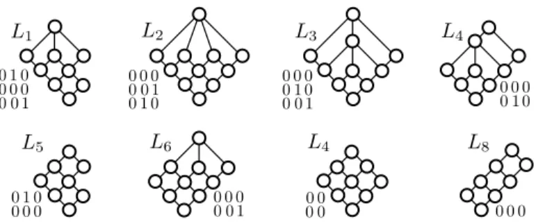
Figure 2. Indecomposable slim semimodular lattices of length 4
for all A ∈ SM. Clearly, all non-square slim matrices and all symmetric slim matrices belong to SM∼, since they belong to one-element ∼T-classes.
Notation. For 0 ≤ k < m ≤ n, let SM(m, n, k) denote the set of slim m-by-n matrices containing exactlykunits. Let SM∼(m, n, k) = SM(m, n, k)∩SM∼. Note that SM∼(m, n, k) = SM(m, n, k) if m < n.
Next, we recall the main result of Cz´edli [5], and supplement it with the statement of Lemma 4.1.
Proposition 4.3 (see [5] for (i) and Lemma 4.1 for (ii)).
(i) There is a bijective correspondence between SM∼ and the set S∞
h=2SSL(h)∼= of isomorphism classes of indecomposable slim semimodular lattices.
(ii) The restriction of the above-mentioned correspondence yields a bijective cor- respondence between SM∼(m, n, k)and SSL(m+n−k)∼=.
Based on Proposition 4.3, it will be sufficient to count the slim matrices.
5. Formulating the main result
Notation. The set of symmetric slim m-by-m matrices that contain exactly k units is denoted by SSM(m, k). If a capital letter, possibly with parameters and superscripts, is used to denote a finite set of matrices, then the size of this set will be denoted by the corresponding lowercase letter. For example, sm∼(m, n, k) =
|SM∼(m, n, k)|and ssm(m, k) =|SSM(m, k)|. We always assume
(5.1) 0≤k < m≤n.
Clearly,
sm∼(m, n, k) =
( sm(m, n, k) + ssm(m, k)
/2, if m=n
sm(m, n, k), if m < n .
(5.2)
Let SM0(m, n, k) and SSM0(m, k) denote the set of those members of SM(m, n, k) and SSM(m, k), respectively, whose first row is zero. Similarly, let SM1(m, n, k) stand for SM(m, n, k)\SM0(m, n, k), and let SSM1(m, k) = SSM(m, k)\SSM0(m, k).
Keeping the general assumption (5.1) in mind, we clearly have
(5.3) sm0(m, n,0) = 1, sm1(m, n,0) = 0, and ssm1(m,0) = ssm1(m,1) = 0.
The main step towards the number of slim semimodular lattices is summarized in the following statement, where (2t−1)!! denotes 1·3·5· · ·(2t−1) = (2t)!/(2t·t!).
As usual in case of empty products, (−1)!! = 1 by definition.
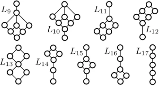
Figure 3. Decomposable slim semimodular lattices of length 4
Lemma 5.1. sm∼(m, n, k)is determined by induction based on (5.1),(5.2),(5.3), and the following six formulas:
sm0(m, n, k) =
m−1 k
· n!
(n−k)!−
m−2 k−1
· n!
(n−k+ 1)!, (5.4)
sm1(m, n, k) =
k−1X
j=0
j!·sm(m−j−1, n−j−1, k−j−1)·(n−j−2), (5.5)
sm(m, n, k) = sm0(m, n, k) + sm1(m, n, k), (5.6)
ssm0(m, k) =
m−1 k
·
bk/2c
X
j=0
k k−2j
·(2j−1)!!, (5.7)
ssm1(m, k) =
k−2X
i=0
(m−3−i)·ssm(m−2−i, k−2−i)× (5.8)
×
bi/2c
X
r=0
i i−2r
·(2r−1)!!, and ssm(m, k) = ssm0(m, k) + ssm1(m, k),
(5.9)
where, in addition to(5.1), we assumek≥1in (5.4)and (5.5), andk≥2in (5.8).
For 2≤h∈N, let ISSL(h) denote the class of indecomposable slim semimodular lattices of lengthh. The corresponding set of isomorphism classes is ISSL(h)∼= = {I(L) :L∈ISSL(h)}, and its size is denoted byNissl(h) =|ISSL(h)∼=|.
Proposition 5.2. The number of indecomposable slim semimodular lattices of lengthhis
(5.10) Nissl(h) =
h−2X
k=0 h−1X
n=h+k
2
sm∼(h+k−n, n, k).
Now, we are ready to formulate our main result.
Theorem 5.3. N(0) = 1 and, forh∈N, N(h) =N(h−1) +
Xh
j=2
Nissl(j)·N(h−j).
Based on Lemma 5.1 and Proposition 5.2, Theorem 5.3 offers an effective way to computeN(h). For comparison, note that there are several papers on counting other particular lattices; for example, see Ern´e, Heitzig and Reinhold [13] and Pawar and Waphare [24]. There are also papers on enumerating all finite lattices of a given sizes, see Heitzig and Reinhold [19] fors≤18, and see the references listed in [19].
The calculation fors= 18 took several days on a parallel supercomputer in 2001.
If we store the previously computed values, then the calculation ofN(h) by com- puter algebra is sufficiently fast. Appropriate programs (Maple 5 and Mathematica 6) are available from the authors’ web sites, where
h, Nissl(h)
:h ≤100 and h, N(h)
: h ≤ 100 are also available. Using a personal computer with Intel Duo CPU 3.00 GHz, 1.98 GHz, and 3.25 GB RAM, it took only four seconds and two minutes, respectively, to obtain the following two values:
N(50) = 15206749438920313735718988921891666957488791414690\
892747031888674≈0.1520674944·1065, and N(100) = 4666300514485158296402274322204901463839367594\
229481848806020032670884439457210266367922\
3692209862830282250013360549818627829410391\
422578476758494039360841845≈0.4666300514·10158. The following table was computed in less than 0.1 seconds:
h 0 1 2 3 4 5 6 7 8 9 10 11 12
Nissl(h) 0 0 1 2 8 39 242 1 759 14 674 137 127 1 416 430 16 006 403 196 400 810 N(h) 1 1 2 5 17 73 397 2 623 20 414 181 607 1 809 104 19 886 032 238 723 606
6. Combinatorial lemmas and proofs
By a permutation matrix we mean a k-by-k square 0,1-matrix satisfying (1•) and containingkunits. The following lemma belongs to folklore.
Lemma 6.1. The number of symmetrick-by-k permutation matrices is
(6.1)
bk/2c
X
j=0
k k−2j
·(2j−1)!!. This number is also the size of the set {σ∈Sk :σ=σ−1}.
Proof. Symmetric permutation matrices correspond to those permutations π on the set {1, . . . , k}that are products of pairwise disjoint transpositions. These are exactly those π ∈Sk that satisfy π=π−1. Express a self-inverse permutation π as π= (u1v1)· · ·(ujvj) where j ∈N0 and{us, vs} ∩ {ut, vt}=∅for s6=t. The order of these transpositions is irrelevant. For a givenj, the first factor in (6.1) says how many ways the fixed points ofπcan be chosen. Letu1 denote one of the 2j non-fixed points. We can choose v1 in 2j−1 ways. Denoting by u2 one of the remaining 2j−2 points, we can choosev2in 2j−3 ways. Continuing the process,
we obtain (2j−1)!!, the second factor in (6.1).
Fori∈ {1, . . . , m}, letei denote them-dimensional column vector with 1 in the i-th entry and zeros elsewhere.
Lemma 6.2. (5.4)holds.
A=
0 0 0 0
0 1 0 0
0 0 0 1
0 0 1 0
A0=
0 0 1 0 0
0 0 0 0 0
0 1 0 0 0
0 0 0 0 1
0 0 0 1 0
, A=k =
0 0 0 1 0 0
0 0 0 0 0 0
0 0 1 0 0 0
1 0 0 0 0 0
0 0 0 0 0 1
0 0 0 0 1 0
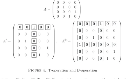
Figure 4. T-operation and B-operation Proof. Since m−1k
= m−2k
+ m−2k−1
and (n−k)!n! −(n−k+1)!n! = (n−k)!n! ·n−k+1n−k , (5.4) is equivalent to
(6.2) sm0(m, n, k) =
m−2 k
· n!
(n−k)!+
m−2 k−1
· n!
(n−k)!· n−k n−k+ 1. Let A ∈ SM0(m, n, k). It consists of k column vectors from {e2, . . . , em} and n−k zero columns. If em is excluded, then no matter how we choose k vectors from{e2, . . . , em−1}, we can do this m−2k
ways, and no matter how we order these k distinct vectors and n−k copies of the zero vector, (n−k)!n! ways, we obviously obtain a matrix in SM0(m, n, k). These possibilities give the first summand in (6.2).
We are left with the more complex case when em occurs inA. In this case, we select onlyk−1 vectors from{e2, . . . , em−1}, and the product of the first two factors of the second summand of (6.2) tells us how many ways we can select and arrange our vectors. However, not all of these arrangements yield a matrix satisfying (5•).
The satisfaction of (5•) depends only on the ordering of em and the n−k zero vectors. For a moment, fix the set of the positions of these n−k+ 1 vectors.
On this set of positions, only one of the possible n−k+ 1 arrangements violates (5•); namely, where em comes first. Hence the ratio of good arrangements to all arrangements is just the third factor in the second summand of (6.2), as desired.
Lemma 6.3. (5.7)holds.
Proof. LetA∈SSM0(m, k). Its first row and, by symmetry, its first column con- tains no unit. Hence (1•) in itself guarantees thatAis a slim matrix. The question is how many ways we can ensure (1•) together with symmetry. The first factor of (5.7) says how many ways we can choose (the indices of) the nonzero columns. By symmetry, the same set of indices is obtained if we consider the nonzero rows. Re- stricting the matrix to these (symmetrically positioned)krows andkcolumns, we obtain a symmetric k-by-kpermutation matrixB. The number of theseB equals
the sum in (5.7) by Lemma 6.1.
Next, we define two matrix operations; see Figure 4. Given an m-by-nmatrix A and i∈ {2, . . . , n}, we define the T-operation betweeni−1and i, abbreviated
to theT-operation ati, as follows. First, we insert a new column with zero entries between the (i−1)-th and the i-th column. In the next step, we insert a new row right before the first row such thei-th entry of the new row is 1 and the rest of its entries are 0. For example, if A is the matrix given in Figure 4, then the T-operation at 3 yieldsA0in Figure 4. (The new elements are the boxed boldface ones.)
By adual T-operationwe mean the composite of a transposition, a T-operation, and a transposition again. Given an m-by-n matrix A and j ∈ {2, . . . , m}, we define the B-operation between j−1 and j, or in short the B-operation at j, as follows. First, we apply a T-operation atj. Then, in the next step, we apply a dual T-operation atj+ 1. For example, ifAis the previous matrix, then the B-operation at 3 yields A=k in Figure 4. Note that A is a symmetric matrix if and only if A=k also is a symmetric matrix . Note also that the set of the new elements looks like a bird (flying to the northwest); this explains the terminology. Let us always assume automatically that
(6.3) 2≤i≤nfor any T-operation, and 2≤j≤mfor any B-operation.
Definition 6.4. A 0,1-matrix A is quasi-slim if it satisfies (1•), (2•), (4•) and (5•). For anm-by-n quasi-slim matrixA, let defA, the defect of A, stand for the largest j ∈N0 such that CornjA containsj units. Observe that defA= 0 if and only ifAis slim.
Lemma 6.5. Let A be an m-by-n matrix. Assume that i ∈ {2, . . . , n} and j ∈ {2, . . . , m}. Let A0 and A=k denote the matrices we obtain from A by performing a T-operation at i and a B-operation at j, respectively. The following assertions hold.
(i) A0determinesA and i. Similarly,A=k determinesAand j.
(ii) A is quasi-slim if and only if A0 is quasi-slim if and only if A=k is quasi-slim.
(iii) If Ais quasi-slim, then A0is slim if and only if 2 + defA≤i≤n, and A=k is slim if and only if 2 + defA≤j≤m.
(iv) If Ais slim, then both A0 and A=k are slim.
Proof. (i) and (ii) are evident. We prove (iii) only for B-operations; the argument for T-operations is almost the same and easier.
Assume first that 2 + defA ≤j ≤m. Let s∈ {1, . . . , m}, let D=k = CornsA=k, and denoteDthe system of those entries ofD=k that belong toA. Ifs≤j, thenD=k has less thansunits since its first row is zero. Hence we may assume s > j. Now D= Corns−2Ahas less thans−2 units sinces−2> j−2≥defA. ThereforeD=k has less thansunits, andA=k is slim.
Next, to show the converse, assumej <2 + defA. Lets= 2 + defA. Since the previously defined D = Corns−2A= CorndefAA hass−2 units, D=k = CornsA=k hassunits. HenceA=kis not slim, proving (iii).
Finally, (iii) together with (6.3) imply (iv).
The next two proofs show the importance of the T- and B-operations.
Lemma 6.6. (5.5)holds.
Proof. Assume A0 ∈ SM1(m, n, k). By Lemma 6.5, there are a unique (m−1)- by-(n−1) quasi-slim matrix A and a unique i ∈ {2, . . . , n−1} such that A0 is obtained fromAby performing a T-operation ati. It suffices to count theseA. Let