Mixed duopolies with advance production

C O R VI N U S E C O N O M IC S W O R K IN G P A PE R S

CEWP 08 /201 8

Mixed duopolies with advance production

by Tamás László Balogh,

Attila Tasnádi

Mixed duopolies with advance production

Tam´as L´aszl´o Balogh

A Matematika ¨Osszek¨ot Egyes¨ulet and Attila Tasn´adi^∗

Department of Mathematics, Corvinus University of Budapest November 30, 2018

Abstract

Production to order and production in advance have been compared in many frame- works. In this paper we investigate a production in advance version of the capacity- constrained Bertrand-Edgeworth mixed duopoly game and determine the solution of the respective timing game. We show that a pure-strategy (subgame-perfect) Nash- equilibrium exists for all possible orderings of moves. It is pointed out that unlike the production-to-order case, the equilibrium of the timing game lies at simultane- ous moves. An analysis of the public firm’s impact on social surplus is also carried out. All the results are compared with those of the production-to order version of the respective game and with those of the mixed duopoly timing games.

Keywords:Bertrand-Edgeworth, mixed duopoly, timing games.

JEL Classification Number: D43, L13.

1 Introduction

We can distinguish between production-in-advance (PIA) and production-to-order (PTO) concerning how the firms organize their production in order to satisfy the consumers’

demand.¹ In the former case production takes place before sales are realized, while in the latter one sales are determined before production takes place. Markets of perishable goods are usually mentioned as examples of advance production in a market. Phillips, Menkhaus, and Krogmeier (2001) emphasized that there are also goods which can be traded both in a PIA and in a PTO environment since PIA markets can be regarded as a kind of spot market whereas PTO markets as a kind of forward market. For example, coal and electricity are sold in both types of environments.

The comparison of the PIA and PTO environments has been carried out in experimen- tal and theoretical frameworks for standard oligopolies.² For instance, assuming strictly increasing marginal cost functions Mestelman, Welland, and Welland (1987) found that in

∗Corresponding author: Attila Tasn´adi, Department of Mathematics, Faculty of Economics, Corvinus University of Budapest, F¨ov´am t´er 8, Budapest H-1093, Hungary. E-mail attila.tasnadi@uni-corvinus.hu.

Tasn´adi gratefully acknowledges the financial support from the Pallas Ath´en´e Domus Sapientiae foun- dation through its PADS Leading Researcher Program.

1The PIA game is also frequently called the price-quantity game or briefly PQ-game.

2We call an oligopoly standard if all firms are profitmaximizers, which basically means that they are privately owned.

an experimental posted offer market the firms’ profits are lower in case of PIA. For more recent experimental analyses of the PIA environment we refer to Davis (2013) and Orland and Selten (2016). In a theoretical paper Shubik (1955) investigated the pure-strategy equilibrium of the PIA game and conjectured that the profits will be lower in case of PIA than in case of PTO. Levitan and Shubik (1978) and Gertner (1986) determined the mixed-strategy equilibrium for the constant unit cost case without capacity constraints.³ Assuming constant unit costs and identical capacity constraints, Tasn´adi (2004) found that profits are identical in the two environments and that prices are higher under PIA than under PTO. Zhu, Wu, and Sun (2014) showed for the case of strictly convex cost functions that PIA equilibrium profits are higher than PTO equilibrium profits. In addi- tion, considering different orders of moves and asymmetric cost functions Zhu, Wu, and Sun (2014) demonstrated that the leader-follower PIA game leads to higher profit than the simultaneous-move PIA game.⁴

Concerning our theoretical setting, the closest paper is Tasn´adi (2004) since we will investigate the constant unit cost case with capacity constraints. The main difference is that we will replace one profit-maximizing firm with a social surplus maximizing firm, that is we will consider a so-called mixed duopoly. We have already considered the PTO mixed duopoly in Balogh and Tasn´adi (2012) for which we found (i) the payoff equivalence of the games with exogenously given order of moves, (ii) an increase in social surplus compared with the standard version of the game, and (iii) that an equilibrium in pure strategies always exists in contrast to the standard version of the game.⁵ In this paper we demonstrate for the PIA mixed duopoly the existence of an equilibrium in pure strategies, (weakly) lower social surplus than in case of the PTO mixed duopoly and the emergence of simultaneous moves as a solution of a timing game.

It is also worthwhile to relate our paper briefly to the literature on mixed oligopolies.

In a seminal paper Pal (1998) investigates for mixed oligopolies the endogenous emergence of certain orders of moves. Assuming linear demand and constant marginal costs, he shows for a quantity-setting oligopoly with one public firm that, in contrast to our result, the simultaneous-move case does not emerge. Matsumura (2003) relaxes the assumptions of linear demand and identical marginal costs employed by Pal (1998). The case of increasing marginal costs in Pal’s (1998) framework has been investigated by Tomaru and Kiyono (2010). In line with our result on the timing of moves B´arcena-Ruiz (2007) obtained the en- dogenous emergence of simultaneous moves for a heterogeneous goods price-setting mixed duopoly timing game. In case of emission taxes Lee and Xu (2018) find that the sequential- move (simultaneous-move) game emerges in the equilibrium of the mixed duopoly timing game under significant (insignificant) environmental externality. There is also an evolv- ing literature on managerial mixed duopolies, for instance, Nakamura (2018) shows that in this case a sequential order of moves emerges in which the private firm with a price contract moves first, while the public firm with a quantity contract moves second.

3Gertner (1986) also derived some important properties of the mixed-strategy equilibrium of the PIA game for strictly convex cost functions. For more on the PIA case see also Bos and Vermeulen (2015), van den Berg and Bos (2017), and Montez and Schutz (2018).

4From the mentioned papers only Zhu, Wu, and Sun (2014) considered sequential orders of moves. For more on standard duopoly leader-follower games we refer to Boyer and Moreaux (1987), Deneckere and Kovenock (1992) and Tasn´adi (2003) in the Bertrand-Edgeworth framework. Furthermore, Din and Sun (2016) extended Zhu, Wu, and Sun (2014) to mixed duopolies.

5We refer the reader also to Bak´o and Tasn´adi (2017) which proves the validity of the Kreps and Scheinkman (1983) result for mixed duopolies by employing the Kreps and Scheinkman tie-breaking rule at the price-setting stage.

The remainder of the paper is organized as follows. In Section 2 we present our frame- work, Sections 3-5 contain the analysis of the three games with exogenously given order of moves, Section 6 solves the timing game, and we conclude in Section 7.

2 The framework

The demand is given by function Don which we impose the following restrictions:

Assumption 1. The demand function D intersects the horizontal axis at quantity a and the vertical axis at price b.D is strictly decreasing, concave and twice continuously differentiable on (0, b); moreover, D is right-continuous at 0, left-continuous at b and D(p) = 0 for allp≥b.

Clearly, any price-setting firm will not set its price above b. Let us denote by P the inverse demand function. Thus, P(q) = D⁻¹(q) for 0< q ≤a, P(0) =b, and P(q) = 0 forq > a.

On the producers side we have a public firm and a private firm, that is, we consider a so- called mixed duopoly. We label the public firm as 1 and the private firm as 2. Henceforth, we will also label the two firms as iand j, wherei, j∈ {1,2}and i6=j. Our assumptions imposed on the firms’ cost functions are as follows:

Assumption 2. The two firms have identical c ∈ (0, b) unit costs up to the positive capacity constraintsk1, k2 respectively.

We shall denote byp^cthe market clearing price and byp^M the price set by a monopolist without capacity constraints, i.e. p^c=P(k1+k2) andp^M = arg max_p∈[0,b](p−c)D(p). In what follows p₁, p₂∈[0, b] andq₁, q₂ ∈[0, a] stand for the prices and quantities set by the firms.

For any firm i and for any quantity qj set by its opponent j we shall denote by p^m_i (q_j) the profit maximizing price on firm i’s residual demand curve D^r_i(p, q_j) = (D(p)−q_j)⁺ with respect to its capacity constraint, i.e. p^m_i (q_j) = arg max_p∈[0,b](p − c) min{D_i^r(p, qj), ki}. Clearly, p^m_i is well defined whenever c < P(qj) and Assumptions 1-2 are satisfied. If c≥P(q_j), then p^m_i (q_j) is not unique, as any price p_i ∈ [0, b] together with quantityq_i= 0 results inπ_i = 0 andπ_icannot be positive. For notational convenience we define p^m_i (qj) by bin case ofc≥P(qj).

For a given quantity q_j we shall denote the inverse residual demand curve of firm i by R_i(·, q_j). In addition, we shall denote by q_i^m(q_j) the profit maximizing quantity on firm i’s inverse residual demand curve subject to its capacity constraint, i.e. q^m_i (qj) = arg max_q∈[0,ki](R_i(q, q_j)−c)q. It can be checked that R_i(q_i, q_j) =P(q_i+q_j) andq^m_i (q_j) = D^r_i (p^m_i (q_j), q_j).⁶

Let us denote byp^d_i(qj) the smallest price for which (p^d_i(q_j)−c) minn

k_i, D

p^d_i(q_j)o

= (p^m_i (q_j)−c)q_i^m(q_j),

whenever this equation has a solution.⁷ Provided that the private firm has ‘sufficient’

capacity, that is max{p^c, c} < p^m₂ (k1), then if it is a profit-maximizer, it is indifferent to

6Note thatD^ri(p^mi (qj), qj)≤kisincep^mi (qj)≥P(ki+qj).

7The equation defining p^d_i(qj) has a solution for anyqj ∈[0, kj] if, for instance,p^m_i (qj)≥max{p^c, c}, which will be the case in our analysis when we refer top^d_i(qj).

whether serving residual demand at price levelp^m₂ (q₁) or selling min{k₂, D p^d₂(q₁)

}at the weakly lower price levelp^d₂(q1). Observe that ifRi(ki, qj) =p^m_i (qj), thenp^d_i(qj) =p^m_i (qj).⁸ We shall denote by ˜q_j the largest quantity for whichq_i^m(˜q_j) =k_iin case ofp^M ≤P(k_i) (i.e.

q^m_i (0) =k_i), and zero otherwise. From Deneckere and Kovenock (1992, Lemma 1) it follows thatp^d_i(·) andp^m_i (·) are strictly decreasing on [˜qj, kj]. Moreover,q_i^m(·) is strictly decreasing on [˜q_j, k_j] and constant on [0,q˜_j], and therefore ˜q_j = inf{q_j ∈[0, a]|q_i^m(q_j)< k_i}is always uniquely defined.

We assume efficient rationing on the market, and thus, the firms’ demands equal

∆i(D, p1, q1, p2, q2) =







D(p_i) if p_i< p_j, T_i(p, q₁, q₂), if p=p_i=p_j (D(p_i)−q_j)⁺ if p_i> p_j,

for all i∈ {1,2}, whereTi stands for a tie-breaking rule. We will consider two sequential- move games (one with the public firm as the first mover and one with the private firm as the first-mover) and a simultaneous-move game. We employ the same tie-breaking rule as Deneckere and Kovenock (1992).

Assumption 3. If the two firms set the same price, then we assume for the sequential- move games that the demand is allocated first to the second mover⁹ and for the simultaneous-move game that the demand is allocated in proportion of the firms’ ca- pacities.

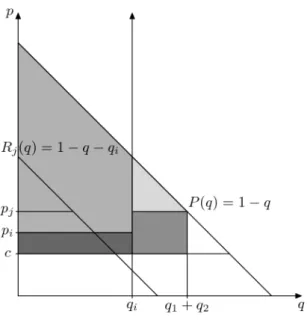
Now we specify the firms’ objective functions. The public firm aims at maximizing total surplus, that is,

π₁(p₁, q₁, p₂, q₂) =

Z min{(D(pj)−q_i)⁺,qj}

0

R_j(q, q_i)dq+

Z min{a,q_i} 0

P(q)dq−c(q₁+q₂)

=

( Rmin{D(p_j),q1+q2}

0 P(q)dq−c(q₁+q₂) if D(p_j)> q_i, Rmin{D(pi),qi}

0 P(q)dq−c(q1+q2) ifD(pj)≤qi, (1) where 0≤p_i≤p_j ≤b. We illustrate social surplus in Figure 1.

The private firm is a profitmaximizer, and therefore,

π₂(p₁, q₁, p₂, q₂) =p₂min{q₂,∆₂(D, p₁, q₁, p₂, q₂)} −cq₂. (2) We divide our analysis into three cases.

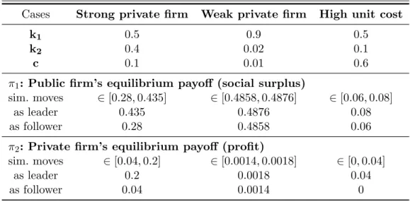
1. Thestrong private firm case, where we assume thatq₂^m(k₁)< k₂ andP(k₁)> c. This means that the private firm’s capacity is large enough to have strategic influence on the outcome and the public firm cannot capture the entire market.

2. The weak private firm case, where we assume that q^m₂ (k₁) = k₂ and P(k₁) > c. In this case the private firm’s capacity is not large enough to have strategic influence on the outcome, but it has a unique profit-maximizing price on the residual demand curve.

8This can be the case ifp^M < P(k1).

9This ensures for the case when the public firm moves first the existence of a subgame perfect Nash equilibrium in order to avoid the consideration of ε-equilibria implying a more difficult analysis without substantial gain.

Figure 1: Social surplus

3. The high unit cost case, where we assume that c≥P(k1). In this case if the public firm produces at its capacity level, then there is no incentive for the private firm to enter the market, because the cost level is too high.

Clearly, the three cases are well defined and disjunct from each other.

We now determine all the equilibrium strategies of both firms for the three possible orderings of moves in each of the three main cases. Within every case we begin with the simultaneous moves subcase, thereafter we focus on the public-firm-moves-first subcase, finally we analyze the private-firm-moves-first subcase. The results are always illustrated with numerical examples. For better visibility, the most interesting equilibria are depicted.

3 The strong private firm case

The following two inequalities remain true for the simultaneous moves and public leader- ship cases.

Lemma 1. Under Assumptions 1-3, q₂^m(k₁)< k₂ and P(k₁)> c we must have in case of simultaneous moves and public leadership that

p^∗₂ ≥p^d₂(q₁^∗) (3)

in any equilibrium (p^∗₁, q^∗₁, p^∗₂, q^∗₂) in which q^∗₁ >0.

Proof. We obtain the result directly from the definition ofp^d₂(q1). For anyq1 ∈[0, k1], the private firm is better off by settingp₂ =p^m₂ (q₁) andq₂ =q₂^m(q₁) than by setting any price p₂ < p^d₂(q₁) and any quantityq₂ ∈[0, k₂].

Lemma 2. Under Assumptions 1-3, q₂^m(k₁) < k₂ and P(k₁) > c we have in case of simultaneous moves and public leadership that

p^∗₂≤p^m₂ (0) = max{P(k₂), p^M} (4) in any equilibrium (p^∗₁, q^∗₁, p^∗₂, q^∗₂).

Proof. Suppose that p^∗₂ > max{P(k₂), p^M}. If p^∗₂ ≤ p^∗₁, then the private firm would be better off by setting price max{P(k2), p^M} and quantity D max{P(k2), p^M}

. If p^∗₂ > p^∗₁, then the private firm serves residual demand, and therefore it could bene- fit from switching to action (p^m₂ (q^∗₁), q₂^m(q₁^∗)), max{P(k₂), p^M}, D max{P(k₂), p^M}

, or (p^∗₁−ε,min{k₂, D(p^∗₁−ε)}), whereεis a sufficiently small positive value. For both cases we have obtained a contradiction.

3.1 Simultaneous moves

For the case of simultaneous moves we have a pure-strategy Nash equilibrium family,¹⁰ which contains profiles where the private firm maximizes its profit on the residual demand choosingp^∗₂ =p^m₂ (q^∗₁) andq₂^∗=q₂^m(q₁^∗), while the public firm can choose any price level not greater than p^d₂(q^∗₁) and produce any non-negative amount up to its capacity. It is worth emphasizing that in case of p^m₂ (q^∗₁) =p^d₂(q^∗₁) the private firm can sell its entire capacity.

Proposition 1 (Simultaneous moves). Let Assumptions 1-3, q₂^m(k1)< k2 and P(k1)> c be satisfied. A strategy profile

(p^∗₁, q^∗₁, p^∗₂, q^∗₂) = (p^∗₁, q^∗₁, p^m₂ (q₁^∗), q^m₂ (q^∗₁)) (5) is for a quantity q₁^∗∈(0, k1] and for any price p^∗₁ ∈

0, p^d₂(q₁^∗)

or for any q₁^∗= 0 and any p^∗₁ ∈[0, b]a Nash-equilibrium in pure strategies if and only if

π1

p^d₂(q^∗₁), q₁^∗, p^m₂ (q^∗₁), q^m₂ (q^∗₁)

≥π1(P(k1), k1, p^m₂ (q₁^∗), q^m₂ (q^∗₁)),¹¹ (6) where there exists a nonempty closed subset Hof [0, k₁]satisfying condition (6).¹² Finally, no other equilibrium in pure strategies exists.

Proof. Assume that (p^∗₁, q^∗₁, p^∗₂, q₂^∗) is an arbitrary equilibrium profile. We divide our anal- ysis into three subcases. In the first case (Case A) we have p^∗₁ = p^∗₂, in the second one (Case B) p^∗₁ > p^∗₂ holds true, while in the remaining case we have p^∗₁ < p^∗₂ (Case C).

Case A:We claim thatp^∗₁ =p^∗₂impliesq^∗₁+q₂^∗=D(p^∗₂). Suppose thatq₁^∗+q₂^∗< D(p^∗₂).

Then¹³because ofp^∗₂ >max{p^c, c}by a unilateral increase in output the public firm could increase social surplus or the private firm could increase its profit; a contradiction. Suppose that q^∗₁+q₂^∗> D(p^∗₂). Then the public firm could increase social surplus by decreasing its output or if q₁^∗ = 0, the private firm could increase its profit by producing only D(p^∗₂); a contradiction.

We know that we must havep^∗₁ =p^∗₂≥p^d₂(q^∗₁) by Lemma 1. Assume thatq^∗₁ >0. Then we must have q^∗₂ = min{k₂, D(p^∗₂)}, since otherwise the private firm could benefit from reducing its price slightly and increasing its output sufficiently (in particular, by setting p₂ = p^∗₂−ε and q₂^∗ = min{k₂, D(p₂)}). Observe thatp^m₂ (0) = p^d₂(0), p^m₂ (q₁) = p^d₂(q₁) for all q₁ ∈[0,q˜₁] and p^m₂ (q₁)> p^d₂(q₁) for all q₁ ∈(˜q₁, k₁].¹⁴ Moreover, it can be verified by the definitions of p^m₂ (q^∗₁) and p^d₂(q^∗₁) that q^∗₁ +k2 ≥ D(p^d₂(q₁^∗)) ≥ D(p^∗₂), where the first inequality is strict if q^∗₁ >q˜₁. Thus,q^∗₁ >q˜₁ is in contradiction with q₂^∗ = min{k₂, D(p^∗₂)}

10Provided that certain conditions hold true.

11Clearly,P(k1)< p^m₂ (q^∗₁), i.e.k1> D(p^m₂ (q₁^∗)) =q^m₂ (q₁^∗) is a necessary condition for (6).

12In particular, there exists a subset [q, k1] ofH.

13Observe that by Lemma 1, the monotonicity of p^d2(·), q^m2 (k1) < k2 and P(k1) > c, we have p^∗2 ≥ p^d₂(q1)≥p^d₂(k1)>max{p^c, c}.

14We recall that ˜qihas been defined afterp^d_i(qj).

since we already know that q^∗₁ +q₂^∗ =D(p^∗₂) in Case A. Hence, an equilibrium in which both firms set the same price and the public firm’s output is positive exists if and only if p^m₂ (q₁^∗) =p^d₂(q₁^∗) (i.e.,q^∗₁ ∈(0,q˜₁)) and (6) is satisfied. This type of equilibrium appears in (5) with q₂^∗=q₂^m(q₁^∗) =k₂.

Moreover, it can be verified that (p^∗₁, q^∗₁, p^∗₂, q^∗₂) = (p^m₂ (0),0, p^m₂ (0), q₂^m(0)) is an equilib- rium profile in pure strategies if and only if

π₁(p^m₂ (0),0, p^m₂ (0), q₂^m(0))≥π₁(P(k₁), k₁, p^m₂ (0), q^m₂ (0)), (7) where we emphasize thatp^m₂ (0) = max{P(k2), p^M}and q^m₂ (0) =D(max{P(k2), p^M}).

Case B: Suppose that p^∗₁ > p^∗₂ ≥ p^d₂(q₁^∗) and D(p^∗₂) > q₂^∗. Then the public firm could increase social surplus by setting price p₁ = p^∗₂ and q₁ = min{k₁, D(p^∗₂)−q^∗₂}; a contradiction.

Assume thatp^∗₁ > p^∗₂ ≥p^d₂(q₁^∗) and D(p^∗₂) =q^∗₂. Then in an equilibrium we must have q^∗₁ = 0, p^∗₂ = p^m₂ (0) and q^∗₂ = q₂^m(0). Furthermore, it can be checked that these profiles specify equilibrium profiles if and only if equation (6) is satisfied.

Clearly,p^∗₁ > p^∗₂ ≥p^d₂(q₁^∗) and D(p^∗₂) < q^∗₂ cannot be the case in an equilibrium since the private firm could increase its profit by producing q₂ =D(p^∗₂) at pricep^∗₂. Finally, by Lemma 1p^∗₂< p^d₂(q^∗₁) cannot be the case either.

Case C: In this case p^∗₂ = p^m₂ (q₁^∗) and q^∗₂ = q₂^m(q₁^∗) must hold, since otherwise the private firm’s payoff would be strictly lower. In particular, if the private firm sets a price not greater than p^∗₁, we are not anymore in Case C; if q₂^∗ > min{D^r₂(p^∗₂, q₁^∗), k2}, then the private firm either produces a superfluous amount or is capacity constrained;

if q^∗₂ < min{D₂^r(p^∗₂, q^∗₁), k₂}, then the private firm could still sell more than q^∗₂; and if q^∗₂ = min{D^r₂(p^∗₂, q₁^∗), k2}, then the private firm will choose a price-quantity pair maxi- mizing profits with respect to its residual demand curve D^r₂(·, q^∗₁) subject to its capacity constraint. In addition, in order to prevent the private firm from undercutting the public firm’s price we must havep^∗₁ ≤p^d₂(q₁^∗).

Clearly, for the given valuesp^∗₁,p^∗₂ andq^∗₂ from our equilibrium profile the public firm has to choose a quantity q₁⁰ ∈[0, k₁], which maximizes functionf(q₁) =π₁(p^∗₁, q₁, p^∗₂, q₂^∗) on [0, k1]. We show that q₁⁰ =q₁^∗ must be the case. Obviously, it does not make sense for the public firm to produce less than q^∗₁ since this would result in unsatisfied consumers.

Observe that for allq₁∈[q^∗₁,min{D(p^∗₂), k₁}]

f(q1) =

Z D(^p∗2)^−q1

0

(R2(q, q1)−c)dq+ Z q1

0

(P(q)−c)dq−c(q1−q₁^∗) =

=

Z D(^p∗2)

0

P(q)dq−D(p^∗₂)c−c(q₁−q₁^∗). (8) Since only −c(q₁ − q^∗₁) is a function of q₁ we see that f is strictly decreasing on [q₁^∗,min{D(p^∗₂), k₁}].

Subase (i):In case of k1 ≤D(p^∗₂) we have already established that q₁^∗ maximizes f on [0, k₁]. Moreover, (p^∗₁, q^∗₁) maximizes π₁(p₁, q₁, p^∗₂, q^∗₂) on [0, p^∗₂)×[0, k₁] since equation (8) is not a function of p^∗₁. Hence, for any p₁ ≤ p^d₂(q₁^∗) such that p₁ < p^∗₂ we have that (p1, q^∗₁, p^m₂ (q₁^∗), q₂^m(q₁^∗)) specifies a Nash equilibrium for any q1 ∈ [0, k1] satisfying k1 ≤ D(p^m₂ (q₁^∗)). However, note that in case ofq₁^∗ ∈[0,q˜1] andp1 =p^d₂(q₁^∗) we are leaving Case C and obtain a Case A Nash equilibrium.

Observe that p^m₂ (k1) > max{p^c, c} implies that k1 < D(p^m₂ (k1)), and therefore we always have Subcase (i) equilibrium profiles. Since D(p^m₂ (·)) is a continuous and strictly

increasing function, interval [qe₁, k₁]∩(0, k₁] determines the set of quantities yielding an equilibrium for Subcase (i).

Subase (ii): Turning to the more complicated case of k₁ > D(p^∗₂), we also have to investigate functionf above the interval [D(p^∗₂), k₁] in which region the private firm does not sell anything at all at price p^∗₂ and

f(q1) =

Z min{^q1,D(^p∗1)}

0

(P(q)−c)dq−cq^∗₂−c(q1−D(p^∗₁))⁺. (9) Observe that we must have P(k₁)< p^∗₂. If the public firm is already producing quantity q1=D(p^∗₂), the private firm does not sell anything at all and contributes to a social loss of cq₂^∗. Therefore, f(q) is increasing on [D(p^∗₂),min{D(p^∗₁), k1}].

Assume that k₁ ≤ D(p^∗₁). Then for any p₁ ≤ p^d₂(q₁^∗) we get that (p₁, q^∗₁, p^m₂ (q₁^∗), q₂^m(q₁^∗)) is a Nash equilibrium if and only if

π1

p^d₂(q^∗₁), q₁^∗, p^m₂ (q₁^∗), q^m₂ (q^∗₁)

≥ π1

p^d₂(q₁^∗), k1, p^m₂ (q^∗₁), q₂^m(q₁^∗)

=

= π1(P(k1), k1, p^m₂ (q₁^∗), q₂^m(q₁^∗)), (10) where the last equality follows from the inequalitiesp^∗₁ ≤P(k1)≤p^∗₂valid for this case and the fact that social surplus is maximized in function of (p₁, q₁) subject to the constraint that the private firm does not sell anything at all if the public firm sets an arbitrary price not greater than P(k1) and producesk1.

Assume thatk₁ > D(p^∗₁). Therefore,f(q) would be decreasing on [D(p^∗₁), k₁]. However, it can be checked that the public firm could increase social surplus by switching to strategy (P(k1), k1) from strategy (p^∗₁, D(p^∗₁)). In addition, any strategy (p1, k1) with p1 ≤P(k1) maximizes social surplus subject to the constraint that the private firm does not sell anything at all. Therefore, p^d₂(q₁^∗), q^∗₁, p^m₂ (q₁^∗), q^m₂ (q₁^∗)

is a Nash equilibrium if and only if condition (6) is satisfied. Comparing equation (10) with equation (6), we can observe that we have derived the same necessary and sufficient condition for a strategy profile being a Nash equilibrium, which is valid for Subcase (ii).

So far we have established that there exists a function g, which uniquely determines the highest equilibrium price as a function of quantity q produced by the public firm.

Clearly, g(q) = p^d₂(q), where the domain of g is not entirely specified. At least we know from Subcase (i) that the domain of gcontains [qe1, k1]. Observe also that the equilibrium profiles of Subcase (i) satisfy condition (6). Let u(q1) = π1 p^d₂(q1), q1, p^m₂ (q1), q₂^m(q1) and v(q₁) = π₁(P(k₁), k₁, p^m₂ (q₁), q₂^m(q₁)). Hence, q₁ determines a Nash equilibrium profile if and only if u(q1) ≥ v(q1). It can be verified that u and v are continuous, and therefore, set H ={q∈[0, k1]|u(q)≥v(q)}is a closed set containing [q, ke 1].

For the illustration of the Nash equilibrium profile mentioned in the statement let D(p) = 1−p,k₁= 0.5,k₂ = 0.4, andc= 0.1. Now the following values can be calculated directly from the exogenously given data: p^c= 0.1,p^m₂ (k1) = 0.3,q^m₂ (k1) = 0.2, p^d₂(k1) = 0.2. Since p^m₂ (k₁)> p^d₂(k₁) we have

(p^∗₁, q₁^∗, p^∗₂, q₂^∗) =

p^∗₁, q₁^∗,1−q₁^∗−c

2 ,1−q₁+c 2

in equilibrium, where q₁^∗ ∈[0,0.5] andp^∗₁ ∈[0,0.2].

In particular, if q^∗₁ = k1 = 0.5 and p^∗₁ = p^d₂(k1) = 0.2, then p^∗₂ = 0.3 and q₂^∗ = 0.2 (see Figure 2). Calculating the social surplus (the sum of dark gray and light gray areas

in Figure 2) and the private firm’s profit (the light gray area indicated by π₂), we obtain π1 = 0.435 andπ2 = 0.04. It is easy to check that for this profile the necessary condition (6) is satisfied.

Figure 2: The strong private firm case - both firms have positive output

Clearly, p^∗₁ and q^∗₁ can vary within the given ranges. Decreasing p^∗₁ results in lower producer surplus for the public firm, but in an equally large increase in consumer surplus.

Thus, payoffs remain the same. Altering q₁^∗ shifts the residual demand curve, and results in varying payoffs. The possible payoff intervals can also be calculated for the example:

π₁∈[0.28,0.435] and π₂ ∈[0.04,0.2].

3.2 Public firm moves first

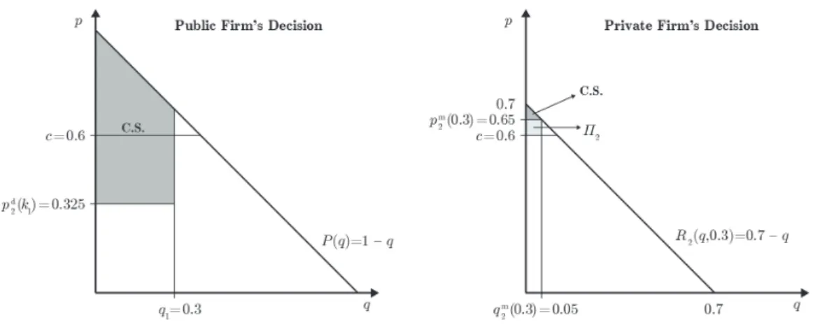
We continue with the case of public leadership. Here, we have a unique family of pure- strategy subgame-perfect Nash equilibria, where the public firm produces its capacity limit at a price not greater than p^d₂(k₁). The private firm serves residual demand and acts as a monopolist on the residual demand curve, as presented in the following proposition.

Proposition 2(Public firm moves first). Let Assumptions 1-3,q₂^m(k₁)< k₂andP(k₁)> c be satisfied. Then the set of SPNE prices and quantities are given by

(p^∗₁, q^∗₁, p^∗₂, q^∗₂) = (p₁, k₁, p^m₂ (k₁), q^m₂ (k₁)) (11) for any p1 ≤p^d₂(k1).

Proof. First, we determine the best reply BR2 = (p^∗₂(·,·), q₂^∗(·,·)) of the private firm.

Observe that the private firm’s best response correspondence can be obtained from the proof of Proposition 1. BR₂(p₁, q₁) =











{(p^m₂ (q₁), q^m₂ (q₁))} ifp₁< p^d₂(q₁);

{(p^m₂ (q₁), q^m₂ (q₁)),(p₁,min{k₂, D(p₁)})} ifp₁=p^d₂(q₁);

{(p₁,min{k₂, D(p1)})} ifp^d₂(q1)< p1 ≤p^m₂ (0);

{(p^m₂ (0), q₂^m(0))} ifp^m₂ (0)< p₁.

Though there are two possible best replies for the private firm to the public firm’s first- period action p^d₂(q1), q1

, in an SPNE the private firm must respond with (p^m₂ (q1), q₂^m(q1)) because otherwise, there will not be an optimal first-period action for the public firm.

Hence, the public firm maximizes social surplus in the first period by choosing pricep^∗₁= p^d₂(k1) and quantityk1. Then the private firm follows with pricep^∗₂=p^m₂ (k1) and quantity q^∗₂ =q₂^m(k₁).

Continuing with the example of linear demand D(p) = 1 − p, we focus on the simultaneous-move outcome, which matches the SPNE emerging in case of public leader- ship. Let the capacities and the unit cost be k₁= 0.5,k₂ = 0.4 andc= 0.1, respectively.

Then the actions associated with the only subgame-perfect Nash equilibrium profile are

(p^∗₁, q₁^∗, p^∗₂, q^∗₂) = (p^∗₁,0.5,0.3,0.2).

wherep^∗₁ ∈[0,0.3]. The social surplus and the private firm’s profit are equal toπ₁ = 0.435 and π2 = 0.04.

3.3 Private firm moves first

Now we consider the case of private leadership. In this case, there exists one type of subgame-perfect Nash equilibria in which the private firm produces on the original demand curve at the highest price level not above its its monopoly price for which it is still of the public firm’s interest to remain on the residual demand curve and produce less than it would produce on the original demand curve. Formally, the private firm sets price

pe2= max{p₂ ∈[c, p^m₂ (0)] | π1(p1, D^r₁(p2,min{D(p₂), k2}), p₂,min{D(p₂), k2})≥ π₁(P(k₁), k₁, p₂,min{D(p₂), k₂})}

in the first stage. The equilibrium profiles with their necessary conditions are given formally in the following proposition and the existence of the price pe₂ is shown in its proof.

Proposition 3 (Private firm moves first). Let Assumptions 1-3, q₂^m(k₁) < k₂ and P(k1) > c be satisfied. The equilibrium actions of the firms associated with an SPNE are the following ones

(p^∗₁, q^∗₁, p^∗₂, q^∗₂) = (p1, D^r₁(ep2,min{D(pe2), k2}),pe2,min{D(pe2), k2}) (12) where p^∗₁ ∈[0,pe₂]can be an arbitrary price; furthermore, p^∗₁ ∈ (pe₂, b]are also equilibrium prices in case of q₁^∗= 0.

Proof. We determine the SPNE of the private leadership game by backwards induction without explicitly referring to the proof of Proposition 1. For any given first-stage action (p₂, q₂) of the private firm the public firm never produces less than min{D₁^r(p₂, q₂), k₁}in the second stage. Moreover, if the public firm does not capture the entire market (i.e. the private firm’s sales are positive), it never produces more than min{D^r₁(p2, q2), k1}. If

π1(p2,min{D₁^r(p2, q2), k1}, p₂, q2)≥π1(P(k1), k1, p2, q2) (13) is satisfied at a price p₂ ∈ [0, b] and a quantity q₂ ∈ (0, k₂], then the private firm, by choosing its first-stage action (p2, q2), becomes a monopolist on the market (in case of q2 ≥ D(p2)) or sells its entire production (in case of q2 < D(p2)) since the public firm

cannot increase social surplus by setting a lower price thanp₂ and it definitely does not set a price abovep2. To be more precise if (13) is satisfied with equality the public firm could also respond with price P(k₁) and quantity k₁; however, as it can be verified later in an SPNE the public firm does not choose the latter response. Clearly, if (13) is violated, the public firm responds with priceP(k1) and quantityk1. Therefore, we getBR1(p2, q2) =











{(p₁, D^r₁(p2, q2)|p1 ≤p2)} ifπ1(p1, D₁^r(p2, q2), p2, q2)> π1(P(k1), k1, p2, q2);

{(p₁, k₁)|p₁ ≤P(k₁)} ifπ₁(p₁, D₁^r(p₂, q₂), p₂, q₂)< π₁(P(k₁), k₁, p₂, q₂);

{(p₁, D^r₁(p2, q2)|p1 ≤p2)} ∪

{(p₁, k1)|p1 ≤P(k1)} ifπ1(p1, D₁^r(p2, q2), p2, q2) =π1(P(k1), k1, p2, q2);

Clearly, the private firm does not set a price below c jointly with a positive quan- tity. Furthermore, the private firm can make positive profits because of q₂^m(k1)< k2 and P(k₁) > c, and therefore it sets a price above c. For any given p₂ > c the private firm will never produce less than min{D₂^r(p₂, k₁), k₂} and the left hand side of (13) is con- stant in q2 on [min{D^r₂(p2, k1), k2},min{D(p₂), k2}], while the profits of the private firm are strictly increasing in q2 on the latter interval. Therefore, the private firm produces q₂ = min{D(p₂), k₂} if it produces at all. Henceforth, we substitute q₂ = min{D(p₂), k₂} in equation (13). Then the private firm would like to set price p^m₂ (0) if (13) is satisfied at this price level, otherwise it sets the highest price still satisfying (13). Note that (13) is definitely satisfied at price p^m₂ (0) if P(k₁) ≥ p^m₂ (0), and otherwise the LHS of (13) is larger than its RHS at price P(k1), the LHS is strictly decreasing and continuous, while the RHS is strictly increasing and continuous on [P(k1), p^m₂ (0)], and therefore if (13) is not satisfied atp^m₂ (0), there exists a unique pricepe∈[P(k₁), p^m₂ (0)) such that (13) is satisfied with equality at price p. In the former case the private firm sets pricee p^m₂ (0), while in the latter case price epin the SPNE.

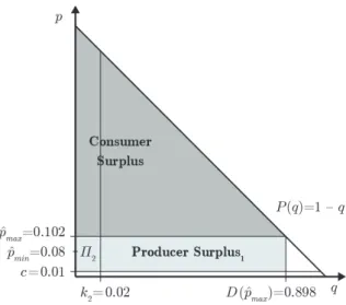
To illustrate Proposition 3 take again the linear demand curve D(p) = 1−p. First, let k1 = 0.5, k2 = 0.4 and c = 0.1 for which pe2 = p^m₂ (0) will be the case. The following values can be calculated directly from the exogenously given data: p^c = 0.1, p^M = 0.55, q^M = 0.45, P(k2) = 0.6. In what follows, in the first stage the private firm will set p^∗₂ =P(k2) = 0.6 and q₂^∗ =k2 = 0.4. It can be checked that for these values the public firm has no incentive to enter the market at stage two. Thus, the actions associated with the SPNE in this case are for allp1 ∈[0,1]:

(p^∗₁, q₁^∗, p^∗₂, q^∗₂) = (p₁,0,0.6,0.4) The respective payoffs are as follows:π₁= 0.28 and π₂ = 0.2.

Second, let k₁ = 0.5, k₂ = 0.4 and c = 0.1 for which pe₂ < p^m₂ (0) will be the case.

Then it can be checked that the public firm will enter the market. Being aware of this, the private firm sets the highest price level (pe₂) at which it can still sell its entire capacity so that the public firm has no incentive to undercut the price level set by the private firm. In this case pe2 = 0.487. The public firm will then satisfy residual demand at pe2 price level, i.e. q^∗₁ = 0.213. The public firm can set its price to any level within [0,0.487]. To sum up, the actions associated with the SPNE in this case are as follows:

(p^∗₁, q^∗₁, p^∗₂, q₂^∗) = (p₁,0.213,0.487,0.4), where p1∈0,0.487. The payoffs areπ1= 0.36 and π2 = 0.116.