Endogenous Timing of Moves in Bertrand-Edgeworth Triopolies

Endogenous Timing of Moves in Bertrand-Edgeworth Triopolies

Attila Tasn´adi^∗

MTA-BCE “Lend¨ulet” Strategic Interactions Research Group, Department of Mathematics, Corvinus University of Budapest^†

December 27, 2012

Abstract

We determine the endogenous order of moves in which the firms set their prices in the framework of a capacity-constrained Bertrand-Edgeworth triopoly. A three- period timing game that determines the period in which the firms announce their prices precedes the price-setting stage. We show for the non-trivial case (in which the Bertrand-Edgeworth triopoly has only an equilibrium in non-degenerated mixed- strategies) that the firm with the largest capacity sets its price first, while the two other firms set their prices later. Our result extends a finding by Deneckere and Kovenock (1992) from duopolies to triopolies. This extension was made possible by Hirata’s (2009) recent advancements on the mixed-strategy equilibria of Bertrand-Edgeworth games.

Keywords:Bertrand-Edgeworth, price leadership, oligopoly, timing games.

JEL Classification Number: D43, L13.

1 Introduction

A challenging question for oligopoly theory and its applications is the determination of the right order of moves because this influences the market structure and its equilibrium be- havior. In this paper we address the timing problem for price-setting games, in particular, within the framework of a homogenous good capacity-constrained Bertrand-Edgeworth triopoly. The key feature of these price-setting games is that the firms may serve less than the demand they are facing. The main difficulty with these models is that one has to con- sider mixed-strategy equilibria since for the interesting cases there is a lack of equilibrium in pure strategies.¹

Deneckere and Kovenock (1992) determined the endogenous order of decisions in a homogeneous good Bertrand-Edgeworth duopoly game with capacity constraints. Their

∗Financial support from the Hungarian Scientific Research Fund (OTKA K-101224) is gratefully ac- knowledged.

†F˝ov´am t´er 8, 1093 Budapest, Hungary (e-mail: attila.tasnadi@uni-corvinus.hu)

1For more on Bertrand-Edgeworth games the reader is referred to Vives (1999).

result was partially generalized from duopolies to oligopolies by Gangopadhyay (1993) who compared the simultaneous-move case with the purely sequential move case, which still did not determine the endogenous order of moves for the oligopolistic case. The main difficulty in solving the timing problem lies in the difficulty of handling the mixed- strategy equilibrium in Bertrand-Edgeworth games. Beckmann (1965), Levitan and Shubik (1972) Vives (1986) and Cheviakov and Hartwick (2005) determined the mixed-strategy equilbrium solutions under quite restrictive assumptions such as linear demand or identical firms. Under more general conditions the mixed-strategy equilibrium has been given in non- closed form by Kreps and Scheinkman (1983), Davidson and Deneckere (1986), Osborne and Pitchik (1986) and Allen and Hellwig (1993) in the duopolistic setting.

The investigation of the triopolistic timing game has been made possible by recent characterizations of the mixed-strategy equilibrium of capacity-constrained Bertrand- Edgeworth triopolies by Hirata (2009) and independently by De Francesco and Salvadori (2010). Based on their characterizations we find that the large-capacity firm will emerge as the endogenous price leader, which extends a result on the duopolistic case obtained by Deneckere and Kovenock (1992). Timing of decisions within the price-setting framework usually results in known forms of price leadership, and therefore, we will also relate our results to the dominant firm model of price leadership.

In general, there is a growing literature on endogenous timing of decisions in oligopolies both in the price-setting and the quantity-setting framework. The first contributions in this direction were made by Gal-Or (1985), Dowrick (1986) and Boyer and Moreaux (1987) in works that compared the outcomes of exogenous timing duopoly games in order to find out whether the leader or the follower has a more advantageous position. The recent literature aims to solve the conflict concerning roles, and determines an endogenous order of moves under certain circumstances. Just to mention some important works from the large number of contributions we refer to Hamilton and Slutsky (1990), Deneckere and Kovenock (1992), van Damme and Hurkens (1999, 2004), Matsumura (1999, 2002), Dastidar and Furth (2005), Yano and Komatsubara (2006, 2012) and von Stengel (2010).

It is worthwile mentioning that another strand of the literature aims to generalize results from the Bertrand-Edgeworth duopoly game with deterministic demand to the case of demand uncertainty. For noteable results in this direction we refer to Hviid (1991), Reynolds and Wilson (2000), de Frutos and Fabra (2011) and Lepore (2012).

The remainder of the paper is organized as follows. Section 2 presents our framework and an important Lemma. Section 3 considers price-setting games with exogenously given orderings of moves. Section 4 determines the solution of our three-period timing game.

Finally, Section 5 contains some concluding remarks.

2 Framework and preliminary result

Suppose that there are three firms on the market, where we shall denote the set of firms by N ={1,2,3}. We assume that the firms have zero unit costs²up to some positive capacity constraints. We shall denote bykithe capacity constraint of firmiand byK =P3

i=1kithe aggregate capacity of the firms. Let the capacity constraints be ordered decreasingly and in order to reduce the number of cases we also assume that the two firms with the smaller

2Since we are considering the production-to-order version of the Bertrand-Edgeworth game (that is, production takes place after the firms’ prices are revealed), the real assumption here is that the firms have identical unit costs.

capacities have identical capacities, i.e. k₁ > k₂ = k₃. We summarize the assumptions imposed on the triopolists’ cost functions below:

Assumption 1. There are three firms on the market with zero unit costs and capacity constraints k1 > k2=k3 >0.

We refer to firm 1 as the large firm and to firms 2 and 3 as the small firms. The demand is given by functionD on which we impose the following restrictions:

Assumption 2. The demand function D intersects the horizontal axis at quantity a and the vertical axis at price b.D is strictly decreasing, concave and twice continuously differentiable on (0, b); moreover, D is right-continuous at 0, left-continuous at b and D(p) = 0 for allp≥b.

Clearly, any price-setting firm will not set its price above b. Let us denote by P the inverse demand function. Thus, P(q) = D⁻¹(q) for 0< q ≤a, P(0) =b, and P(q) = 0 forq > a. In addition, we shall denote byp^c the market clearing price, i.e. p^c=P(K).

Furthermore, we ensure that every firm will be active on the market by the next assumption:

Assumption 3. We assume thatK−k₃ < a.

Letpi ∈[0, b] be the price decision of firmi∈N andti∈ {1,2,3}be the time period in which firmiannonces its price. In the first stage firms choose a time period for announcing their prices and in the second stage firms set their prices (already knowing in which period their opponents set their prices). The market opens after all firms have set their prices.

This type of timing game is referred to as a timing game with observable delay (Hamilton and Slutsky, 1990). Of course, three periods are necessary and sufficient to allow for all possible orderings of moves in case of a triopoly.³

We have to specify a demand-allocating mechanism as a function of price and timing decisions made by the firms. In case of price ties we will assume that the demand is allocated first to firms announcing their prices in an earlier time period. This distinction ensures that we do not have to consider followers slightly undercutting the earlier movers’

prices. Otherwise, the subgames will not always have an equilibrium and we would need to investigate ε-equilibrum solutions. Hence, assuming efficient rationing of consumers, the demand faced by a price-setting firm i∈N is given by

∆i(t,p) =



D(pi)− X

j∈N,pj<pi

kj− X

j∈N,pj=pi,tj<ti

kj





+

ki

P

j∈N,p_j=pi,tj=tikj

.

Thus, firm i∈N makesπi(t,p) =pimin{k_i,∆i(t,p)} profit.

We shall denote by p^m_i the unique revenue maximizing price on the residual demand curveD_i^r(p) = (D(p)−K+k_i)⁺and byq_i^mthe corresponding unique revenue maximizing output on the inverse residual demand curve P_i^r, i.e. p^m_i = arg maxp∈[0,b]pD^r_i (p) and q^m_i = arg max_q∈[0,a]qP_i^r(q) for any i∈ N. Of course, q^m_i = D^r_i (p^m_i ). Clearly, p^c and p^m_i are well defined whenever Assumptions 1-3 are satisfied. Furthermore, it can be checked thatp^m₁ > p^m₂ =p^m₃ because of Assumptions 1-3. Letπi =π^r_i (p^m_i ), whereπ^r_i(p) =pD^r_i (p).

Note that Assumption 3 also ensures thatp^m_i >0 and πi>0.

3The special triopolistic case of only two possible periods has been considered in Tasn´adi (2010). How- ever, at least three periods are needed to allow for the emergence of all possible orderings.

If k_i ≤ q_i^m, then we will say that firm i∈ N has scarce capacity, while otherwise we will say that firm i ∈ N has sufficient capacity. Note that a firm with scarce capacity will be eager to produce at its capacity limit. It can be verified that condition k_i ≤ q_i^m is equivalent to p^c ≥ p^m_i . Let us denote by p^d_i ∈ [0, p^m_i ] the smallest price for which p^d_i min{k_i, D p^d_i

}=p^m_i D^r_i (p^m_i ) whenever this equation has a solution, which is the case, for instance, if firmihas sufficient capacity (implyingp^c< p^d_i < p^m_i ). At pricep^d_i firmiis indifferent to whether serving residual demand at price levelp^m_i or selling min{k_i, D p^d_i

} at the lower price level p^d_i. We will need the following Lemma established for the two firm case by Deneckere and Kovenock (1992) and stated by Hirata (2009) for the triopolistic case.

Lemma 1. Suppose that firm iand j have both sufficient capacity and that Assumptions 1, 2 and 3 are satisfied. If i < j, then p^d_i ≥p^d_j. In addition, if ki > kj, then p^d_i > p^d_j.

3 Exogenously given order of moves

In this section we investigate a variation of the capacity-constrained Bertrand-Edgeworth game with three firms in which the firms can announce their price decisions in one of three subsequent periods. The two-stage game with just two firms has been investigated by Deneckere and Kovenock (1992). They found for the duopolistic case with identical unit costs that the large capacity firm moves first, while the small capacity firm second.⁴ Re- cent characterizations of the mixed-strategy equilibrium of capacity-constrained Bertrand- Edgeworth oligopolies by Hirata (2009) and by De Francesco and Salvadori (2010) make it possible to extend Deneckere’s and Kovenock’s (1992) result from duopolies to triopolies.

Taking Assumption 1 and that the firms can set their prices in three periods into consideration, we have to investigate six different games with exogenously given orderings of moves:

(i) The large firm is the single exogenously given first mover, (ii) the large firm is the single exogenously given last mover,

(iii) one of the small firms is the single exogenously given first mover and the other two firms move simultaneously,

(iv) one of the small firms is the single exogenously given final mover and the other two firms move simultaneously,

(v) a small firm is the exogenously given first mover, the large firm the exogenously given second mover and the other small firm the exogenously given third mover,

(vi) the three firms move in the same period.

Case (vi) leads to the simultaneous-move price-setting game analyzed by Hirata (2009) and De Francesco and Salvadori (2010). If the simultaneous-move game has an equilibrium in pure strategies, then we know that firms make either zero profits or produce all at their capacity limits in a pure-strategy equilibrium, in which case it can be checked that for any ordering of moves we will have the same outcome in cases (i)-(vi). Hence, the timing game is only of real interest if the simultaneous-move price-setting game does not have an equilibrium in pure strategies, i.e Assumption 4 is satisfied.

4They also investigated the case of different unit costs.

Assumption 4. p^m₁ > p^c.

We know from Hirata (2009) and De Francesco and Salvadori (2010) for case (vi) that firm 1’s expected profit equalsπ₁, while firm 2’s and 3’s expected profits equalp^d₁k₂ =p^d₁k₃ under our assumptions. We will treat cases (i)-(v) in separate propositions.

Proposition 1. Under efficient rationing and Assumptions 1-4 if the large firm is the ex- ogenously given first mover, then the unique subgame-perfect equilibrium prices and profits are given by

(p^∗₁, p^∗₂, p^∗₃) = (p^m₁ , p^m₁ , p^m₁ ) and (π₁^∗, π₂^∗, π^∗₃) = (π₁, p^m₁ k₂, p^m₁k₃).

Proof. Clearly, firm 1 sets pricep₁∈[p^d₁, b). Suppose thatp_i > p₁for at least one small firm i∈ {2,3}. If p_i > p_j, where j denotes the other small firm (i6=j and i, j∈ {2,3}), then firm i would not earn more profit than πi =p^d_iki, which is less than p^d₁ki ≤p1ki. Hence, firm i would benefit from switching to price p₁. Switching to price p₁ is also beneficial if p₂ = p₃ > p₁ and the small firms do not sell anything at all. If the small firms face positive residual demand at price p2 = p3 > p1 and the small firms are moving in the same period, then both small firms would benefit from unilaterally undercutting the other small firm’s price. If the small firms face positive residual demand at price p₂ =p₃ > p₁ and the small firms move in different periods, then the first moving small firm would serve residual demand, and therefore it would be better of by setting pricep₁.

From the previous paragraph we know that the small firms do not set prices abovep₁, and therefore the large firm faces residual demand at pricep1. Hence, by maximizing profits with respect to its residual demand curce it sets pricep^m₁ . Therefore, in any possible pure- strategy equilibrium the small firms match the large firm’s price,⁵ i.ep₂ =p₃=p₁, and it can be checked that this price profile corresponds to an equilibrium in pure strategies.

Proposition 1 delivers a partial game-theoretic microfoundation of Forchheimer’s model of dominant firm price leadership in case of a special exogenously given ordering of moves.

We will see later that the ordering assumed in Proposition 1 can be endogenized.

Turning to case (ii) in which the large firm is the sole last mover, we will see that if the large firm is indifferent between matching a small firm’s price or serving residual demand, then in a subgame-perfect equilibrium it has to serve residual demand, and thus sets a higher price than the small firms. As it will be evident from the proof of Proposition 2, the definition of the subgame-perfect Nash equilibrium implies that this can be the only possible response of the large firm although the small firms cannot enforce in stage two that the large firm will not match their price. Anyway to overcome this kind of uncertainty the small firms could enforce an outcome close to the one stated in Proposition 2 by setting a slightly lower price than either p^d₁ orp^u₁, wherep^u₁ ∈(p^d₁, p^m₁ ] is defined byp^u₁min

k1,(D(p^u₁)−k2)⁺ =π1.⁶ This latter defensive behavior would result in an ε-equilibrium on the market.

Proposition 2. Under efficient rationing and Assumptions 1-4 if the large firm is the exogenously given sole last mover, we have to distinguish between the two main cases specified below.

5More precisely, this holds true unlessp1 > P(k2+k3). However, firm 1 will definitely not set a price aboveP(k2+k3) since then the small-capacity firms will not set a price higher thanp1, and thus, firm 1 will not sell anything at all.

6Pricep^u1 can be interpreted as the price at which the large-capacity firm is indifferent between serving residual demand or being undercut by only one small-capacity firm.

1. Ifk₁ ≤D(p^d₁)−k₂, then the subgame-perfect equilibrium prices and profits are given by

(p^∗₁, p^∗₂, p^∗₃) = (p^m₁ , p^d₁, p^d₁) and (π^∗₁, π₂^∗, π₃^∗) = (π₁, p^d₁k₂, p^d₁k₃) for any ordering of moves of the small firms.

2. Ifk1 > D p^d₁

−k2 and

(a) the small firms are moving simultaneously, then we have two possible subgame- perfect equilibria with associated equilibrium prices and profits given by

(p^∗₁, p^∗₂, p^∗₃) = (p^m₁ , p^d₁, p^u₁) and (π₁^∗, π₂^∗, π^∗₃) = (π₁, p^d₁k₂, p^u₁k₃), and (p^∗₁, p^∗₂, p^∗₃) = (p^m₁ , p^u₁, p^d₁) and (π₁^∗, π₂^∗, π^∗₃) = (π1, p^u₁k2, p^d₁k3);

(b) firm 2 is the sole first mover, then the subgame-perfect equilibrium prices and profits are given by

(p^∗₁, p^∗₂, p^∗₃) = (p^m₁ , p^u₁, p^d₁) and (π^∗₁, π^∗₂, π₃^∗) = (π₁, p^u₁k₂, p^d₁k₃);

(c) firm 3 is the sole first mover, then the subgame-perfect equilibrium prices and profits are given by

(p^∗₁, p^∗₂, p^∗₃) = (p^m₁ , p^d₁, p^u₁) and (π^∗₁, π^∗₂, π₃^∗) = (π1, p^d₁k2, p^u₁k3).

Proof. Since firm 1 never sets a price belowp^d₁, the lowest price firms 2 and 3 might set in an equilibrium is p^d₁. Observe that in a pure-strategy subgame-perfect equilibrium at least one of the two small firms must set price p^d₁, since otherwise firm 1 will not set a higher price than the larger one of the two small firms’ prices, and therefore either the small firm setting the highest price would benefit from switching to pricep^d₁ or one of the small firms could benefit from a unilateral price decrease.

Suppose in case of k1 < D(p^d₁)−ki that small firm i sets price p^d₁, while the other small firm j sets a price pj above p^d₁. Then firm 1 would be better off by setting a price beweenp^d₁ andp_j, since at prices slightly higher thanp^d₁ (but lower thanp_j) it can sell its entire capacity and make more profits than π1. Thus, firm j makes π^r_j(pj) profits, which is less than p^d₁k_j; a contradiction. Hence, in case of k₁ < D(p^d₁)−k_i the two small firms set pricep^d₁ if their are moving simultaneously or sequentially before the large firm, which sets pricep^m₁ .

In contrast to the previous case in case of k₁ ≥ D(p^d₁) −k_i firm j could set its first-stage price to p^u₁ because maximizing profits with respect to the demand function D(p) −ki within interval

p^d₁, p^u₁

would not result in higher profits than π1 for the large firm. However, it has to be verified that there exists a value p^u₁ ∈

p^d₁, p^m₁ sat- isfying p^u₁min

k₁,(D(p^u₁)−k₂)⁺ = π₁. Let f(p) = pmin

k₁,(D(p)−k₂)⁺ . Since k₁ ≥ D(p^d₁)−k_i it can be verified that f(p^d₁) ≤ π₁ = p^d₁min

k₁, D p^d₁ , f⁰(p) > 0 on p^d₁, p^m₁

andf(p^m₁ )> π₁=p^m₁ min

k₁,(D(p^m₁ )−k₂−k₃)⁺ . Hence, there exists a unique p^u₁ ∈

p^d₁, p^m₁

satisfyingf(p^u₁) =π1. Obsevere thatp^u₁ =p^d₁ if and only if k1 =D(p^d₁)−ki, and therefore in this special case the two small firms will set both price p^d₁. We conclude that in case ofk₁ > D(p^d₁)−k_i we obtain two asymmetric subgame-perfect equilibria if the two small firms move simultaneously and one subgame-perfect equilibrium if the two small firms move sequentially. It can be checked that the resulting strategy profiles determine the pure-strategy subgame-perfect Nash equilibria stated in the proposition.

The result of Proposition 2 is analogous to case (c) of Theorem 3 in Deneckere and Kovenock (1992) in the sense that the small firms set low prices so that they will not be undercut by the large firm.

We continue our analysis with investigating the case in which a small firm’s move is followed by a simultaneous move of the large firm and the other small firm.

Proposition 3. Under efficient rationing and Assumptions 1-4 if one of the small firms, say firm 3, is the exogenously given first mover and the other two firms move simultane- ously, then the subgame-perfect equilibrium prices and expected profits are given in case of k₁≤D(p^d₁)−k₂ by

(p^∗₁, p^∗₂, p^∗₃) = (X₁^∗, X₂^∗, p^d₁) and (Eπ₁^∗, Eπ₂^∗, π^∗₃) = (π₁, p^d₁k₂, p^d₁k₃), and in case of k₁ > D(p^d₁)−k₂ by

(p^∗₁, p^∗₂, p^∗₃) = (X₁^∗, X₂^∗, p^d₁) and (Eπ^∗₁, Eπ₂^∗, π₃^∗) = (π1, p^u₁k2, p^d₁k3),

where the independent random variables X₁^∗, X₂^∗ describing the prices set by firms1and 2 are distributed according to the mixed-strategy profile (ϕ^∗₁, ϕ^∗₂), which constitutes a mixed- strategy equilibrium of a Bertrand-Edgeworth duopoly game with demand function(D(p)− k₃)⁺.⁷

Proof. By the exogenously given ordering of moves firm 3 sets price p₃ ∈ [0, b] in stage 1, and thereafter, firms 1 and 2 play a simultaneous-move Bertrand-Edgeworth duopoly game with respect to the demand function

D(p) =e

(D(p)−k3)⁺ ifp > p3 and D(p) ifp≤p₃,

which is discontinuous at p₃ if p₃ ∈ [0, b). The subgame has an equilibrium (ϕ₁, ϕ₂) in mixed strategies by Osborne and Pitchik (1986).⁸ Let p_i = sup supp(ϕi) and p_i = inf supp(ϕ_i) for each i∈ {1,2}.

Since any price p₁ < p^d₁ is dominated by price p^m₁ for firm 1 we must have p

1 ≥ p^d₁. Hence, firm 3 will not set its pricep₃ below p^d₁ in a subgame-perfect equilibrium in stage 1, because otherwise it would be better off by setting a price betweenp3 and p^d₁.

Assume that p3 ≥ p^m₁ . Suppose that p₁ > p3 or p₂ > p3 for which case we consider two subcases. First, if p_i > p_j, where i, j∈ {1,2} and i6=j, then firmi’s expected profit equalsπ_i^r(p_i), which is less thanπ^r_i (p^m_i ), and thereforep_i > p_j cannot be the case. Second, suppose thatp₁=p₂. Observe that both equilibrium strategiesϕ1 andϕ2 cannot have an atom at price p₁ =p₂, since otherwise both firms could benefit from unilaterally shifting the probability mass from pricep₁ =p₂to a price slightly belowp₁ =p₂. Thus, we see that the strategy of at most one firm, say firm i∈ {1,2}, can have an atom at pricep₁ =p₂, and therefore its expected profit equals π_i^r(p_i) < π^r_i(p^m_i ). Hence, p₁ = p₂ > p₃ cannot be the case if (ϕ1, ϕ2) is an equilibrium of the subgame. So far we obtained that in case of p3 ≥ p^m₁ we must have p₁ ≤ p3 and p₂ ≤ p3. However, then firm 3 serves its residual

7Henceforth in this section, we emphasize that we have determined the firms’ nondeterministic expected profits by writingEπi, whereas we simply writeπi if profits are deterministic.

8Osborne and Pitchik (1986) mention the case of discontinuous, but left-continuous demand functions in Section 5. For recent advancements on the mixed-strategy equilibrium of the Bertrand-Edgeworth duopoly game we refer to Bagh (2010).

demandD^r₃(p₃), which is strictly dominated by a pricep^d₁−εfor a sufficiently smallε >0.

Therefore, firm 3 never sets a price greater than or equal to p^m₁ .

We have already shown that in the first stage firm 3 selects a price from interval [p^d₁, p^m₁ ).

Assume that firm 3 sets pricep₃=p^d₁. In determining the equilibrium of the subgame, we consider the modified Bertrand-Edgeworth duopoly game with capacity constraints k1 >

k₂ and demand function (D−k₃)⁺, which by Deneckere and Kovenock (1992, Theorem 1) has a unique equilibrium in non-degenerate mixed strategies for which [p

1, p₁] = [p

2, p₂] = [p^d₁, p^m₁ ] ifk₁ ≤D(p^d₁)−k₂, and [p

1, p₁] = [p

2, p₂] = [p^u₁, p^m₁] if k₁ > D(p^d₁)−k₂. Moreover, the expected profits of firms 1 and 2 equalπ1andp₂k2, respectively. In addition, only price p^m₁ is played with positive probability by firm 1. Since (D−k₃)⁺ =De for prices greater thanp^d₁, pricep^d₁ will be played with probability zero and the second movers cannot achieve higher profits by unilaterally switching to price p^d₁, the mixed-strategy equilibrium of the modified game will also be a mixed-strategy equilibrium of our subgame.⁹ Moreover, it has to be the unique equilibrium of the subgame by the way how the mixed-strategy equilibrium has to be calculated.¹⁰

Finally, we turn to the case ofp₃∈ p^d₁, p^m₁

. Suppose that firm 3 can achieve a higher profit by setting pricep3 ∈ p^d₁, p^m₁

than by setting pricep^d₁, where the latter price results in p^d₁k3 profits. We divide our analysis into two subcases: (a) p₁ > p3 and (b) p₁ ≤ p3. In Subcase (a) we must have p₂ ≤p₁, since otherwiseπ₂(ϕ₁, p₂, p₃) =π₂^r(p₂)≤π₂^r(p^m₂ ) = p^d₂k2 < p^d₁k2, which cannot be the case in an equilibrium. Therefore, it follows thatp₁ =p^m₁ , which in turn implies that we cannot have p₂ > p^d₁, since otherwise firm 1 would benefit from switching to p1 ∈(p^d₁,min{p

2, p3}) from ϕ1. Hence, we must have p₂ =p^d₁, and thus p₁ = p^d₁. Employing our assumption that firm 3 is better off by setting a price above p^d₁ than by setting price p^d₁, we obtain that π3(ϕ1, ϕ2, p3) > p^d₁k3 =p^d₁k2 =π2(ϕ1, ϕ2, p3).¹¹ However, π2(ϕ1, p3, p3)≥π3(ϕ1, ϕ2, p3)> π2(ϕ1, ϕ2, p3), where the first inequality follows from the tie-breaking rule, is in contradiction with (ϕ₁, ϕ₂) constituting an equilibrium of the subgame. This means that in Subcase (a) firm 3 sets price p^d₁. Turning to Subcase (b), it can be verified that p₁ ≤p3 impliesp₂ ≤p3, an therefore setting price p3 is worse than setting pricep^d₁for firm 3. Concerning both subcases, we conclude that the first stage equilibrium action of firm 3 is p^∗₃=p^d₁.

From Proposition 3 we see that the small firm moving first has to set a lower price and that the other small firm could be better off.

Now we shall turn to the case in which the simultaneous moves of the large firm and a small firm is followed by the move of the other small firm.

Proposition 4. Under efficient rationing and Assumptions 1-4 if one of the small firms, say firm 3, is the exogenously given last mover and the other two firms move simul- taneously, then the subgame-perfect equilibrium prices and profits are given in case of k₁≤D(p^d₁)−k₂ by

(p^∗₁, p^∗₂, p^∗₃) = (X₁^∗, X₂^∗, Emax{X₁^∗, X₂^∗}) and (Eπ₁^∗, Eπ^∗₂, Eπ₃^∗) = (π1, p^d₁k2, Emax{X₁^∗, X₂^∗}k₃),

9Since D(pe ^d1) > (D−k3)⁺(p^d1) and k1 > (D−k3)⁺(p^d1) in case of k1 > D(p^d1)−k2, it should be emphasized that firm 1 still makes onlyπ1 profit when setting pricep^d₁.

10See Kreps and Scheinkman (1983), Osborne and Pitchik (1986) and Deneckere and Kovenock (1992).

11For the last equality we need thatϕ1 does not have an atom at pricep^d1, which can be shown easily by contradiction.

and in case of k₁ > D(p^d₁)−k₂ by

(p^∗₁, p^∗₂, p^∗₃) = (X₁^∗, X₂^∗, Emax{X₁^∗, X₂^∗}) and (Eπ₁^∗, Eπ^∗₂, Eπ₃^∗) = (π1, p^u₁k2, Emax{X₁^∗, X₂^∗}k₃),

where the independent random variablesX₁^∗, X₂^∗ describing the prices set by firms1 and2, respectively, are distributed according to the mixed-strategy profile (ϕ^∗₁, ϕ^∗₂), which consti- tutes a mixed-strategy equilibrium price profile of a Bertrand-Edgeworth duopoly game with demand function (D(p)−k₃)⁺. In addition, we know that p^d₁k₃ < Emax{X₁^∗, X₂^∗}k₃ <

p^m₁ k3 or p^u₁k3 < Emax{X₁^∗, X₂^∗}k₃ < p^m₁ k3 depending on the case.

Proof. Firm 3 serves its residual demand D^r₃ in stage 2 if p₃ > max{p₁, p₂}. Since firm 1 never sets a price below p^d₁ and p^m₃ D^r₃(p^m₃ ) = p^d₃k3 < p^d₁k3 firm 3 never sets a price higher than max{p₁, p₂}. Hence, firms 1 and 2 face demand curve (D(p)−k₃)⁺ in stage 1. Finally, by taking the results on Bertrand-Edgeworth duopolies (e.g. Deneckere and Kovenock, 1992) into consideration, we obtain the statements of the proposition.

Observe that the small firm being the follower is better off than the other small firm moving simultaneously with the large firm under the Assumptions of Proposition 4.

Finally, we turn to the case in which the large firm moves between the two small firms.

Proposition 5. Under efficient rationing and Assumptions 1-4 if a small firm, say firm 3, is the exogenously given first mover, the large firm the exogenously given second mover and the other small firm the exogenously given third mover, then we have to distinguish between the following two cases.

1. Ifk₁ ≤D(p^d₁)−k₂, then the subgame-perfect equilibrium prices and profits are given by

(p^∗₁, p^∗₂, p^∗₃) = (p^m₁ , p^m₁ , p^d₁) and (π₁^∗, π₂^∗, π^∗₃) = (π₁, p^m₁ k₂, p^d₁k₃).

2. Ifk₁ > D p^d₁

−k₂, then the subgame-perfect equilibrium prices and profits are given by

(p^∗₁, p^∗₂, p^∗₃) = (p^m₁ , p^m₁ , p^u₁) and (π^∗₁, π^∗₂, π₃^∗) = (π₁, p^m₁ k₂, p^u₁k₃).

Proof. Clearly, in period 2 firm 1 will never set a price belowp^d₁ and then the same holds true for firm 2 because of the employed tie-breaking rule. Therefore, firm 3 will neither set a price p₃ below p^d₁, since otherwise it would be better off by setting a price between p₃ and p^d₁. For a similar reason in a subgame-perfect equilibrium firm 3 does not serve its residual demand (which would happen if it sets one of the highest prices) since it would be better off by setting price p^d₁−ε, whereεis a sufficiently small positive value.

Observe that in a subgame-perfect equilibrium p₂, the price set by firm 2, cannot be higher than firm 1’s price because this would imply that either firm 2 or firm 3 must serve residual remand. However, serving residual demand can be avoided by setting pricep^d₁ in case of firm 2 and by setting price p^d₁ −ε in case of firm 3, which would result in more profits for the respective small firm. Hence, firm 1 has to serve residual demand and firm 3 sets the highest possible price in period 1, which still does not result in serving its residual demand. Observe that therefore the same two cases as in Propositions 2-4 emerge. Thus, firm 3 either sets price p^d₁ orp^u₁, firm 1 set price p^m₁ and firm 2 follows with price p^m₁ .

4 Endogenous order of moves

In this section we determine the ordering in which the firms announce their price decisions.

First, the firms decide whether they make their price announcements in period 1,2 or 3.

Second, observing when the other firms have set their prices, the firms play the selected price-setting game corresponding to cases (i)-(vi). That is, a ‘game with observable delay’

is played in the terminology of Hamilton and Slutsky (1990).

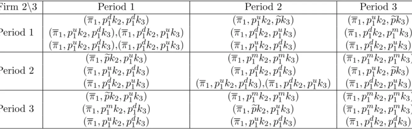
Based on Tables 1 and 2, containing the equilibrium payoffs described in Propositions 1-5, we can determine the equilibrium timing decisions of the firms. The two different tables correspond to the case distinctions made in Propositions 2-5. In both tables the row player is firm 2, the column player is firm 3 and the three rows of each cell of the table correspond to the respective timing decision of firm 1. In addition, Table 2 contains two entries in some rows of some cells because Proposition 2 allows for two possible equilibria in case ofk1> D(p^d₁)−k₂. In both tablespestands for the expected price of the small-capacity firm when playing a mixed-strategy equilibrium according to Proposition 3.

Firm 2\3 Period 1 Period 2 Period 3

(π1, p^d₁k2, p^d₁k3) (π1, p^d₁k2,pke 3) (π1, p^d₁k2,pke 3) Period 1 (π₁, p^d₁k₂, p^d₁k₃) (π₁, p^d₁k₂, p^d₁k₃) (π₁, p^d₁k₂, p^m₁ k₃)

(π₁, p^d₁k₂, p^d₁k₃) (π₁, p^d₁k₂, p^d₁k₃) (π₁, p^d₁k₂, p^d₁k₃) (π₁,pke ₂, p^d₁k₃) (π₁, p^m₁ k₂, p^m₁ k₃) (π₁, p^m₁ k₂, p^m₁ k₃) Period 2 (π1, p^d₁k2, p^d₁k3) (π1, p^d₁k2, p^d₁k3) (π1, p^d₁k2,pke 3)

(π₁, p^d₁k₂, p^d₁k₃) (π₁, p^d₁k₂, p^d₁k₃) (π₁, p^d₁k₂, p^d₁k₃) (π1,pke 2, p^d₁k3) (π1, p^m₁ k2, p^m₁ k3) (π1, p^m₁ k2, p^m₁ k3) Period 3 (π₁, p^m₁ k₂, p^d₁k₃) (π₁,pke ₂, p^d₁k₃) (π₁, p^m₁ k₂, p^m₁ k₃) (π1, p^d₁k2, p^d₁k3) (π1, p^d₁k2, p^d₁k3) (π1, p^d₁k2, p^d₁k3)

Table 1: Timing in case of k1 ≤D(p^d₁)−k2.

Firm 2\3 Period 1 Period 2 Period 3

(π₁, p^d₁k₂, p^d₁k₃) (π₁, p^u₁k₂,pke ₃) (π₁, p^u₁k₂,pke ₃) Period 1 (π1, p^u₁k2, p^d₁k3),(π1, p^d₁k2, p^u₁k3) (π1, p^d₁k2, p^u₁k3) (π1, p^d₁k2, p^m₁ k3)

(π₁, p^u₁k₂, p^d₁k₃),(π₁, p^d₁k₂, p^u₁k₃) (π₁, p^u₁k₂, p^d₁k₃) (π₁, p^d₁k₂, p^u₁k₃) (π₁,pke ₂, p^u₁k₃) (π₁, p^m₁ k₂, p^m₁ k₃) (π₁, p^m₁ k₂, p^m₁ k₃) Period 2 (π₁, p^u₁k₂, p^d₁k₃) (π₁, p^d₁k₂, p^d₁k₃) (π₁, p^u₁k₂,pke ₃)

(π1, p^d₁k2, p^u₁k3) (π1, p^u₁k2, p^d₁k3),(π1, p^d₁k2, p^u₁k3) (π1, p^d₁k2, p^u₁k3) (π1,pke 2, p^u₁k3) (π1, p^m₁ k2, p^m₁ k3) (π1, p^m₁ k2, p^m₁ k3) Period 3 (π1, p^m₁ k2, p^d₁k3) (π1,pke 2, p^u₁k3) (π1, p^m₁ k2, p^m₁ k3) (π₁, p^u₁k₂, p^d₁k₃) (π₁, p^u₁k₂, p^d₁k₃) (π₁, p^d₁k₂, p^d₁k₃)

Table 2: Timing in case of k1 > D(p^d₁)−k2.

Checking both tables, we can see that firm 1 achieves the same expected profit in each case. Studying both tables carefully, we obtain the following subgame-perfect equilibria of the three-period timing game.

Theorem 1. Under efficient rationing and Assumptions 1-4 the timing game, in which the three firms can select between three periods to set their prices and thereafter (already knowing in which period the three firms will set their prices) the firms set their prices, has the following two types of subgame-perfect equilibria:

1. The large firm moves before the small firms and all of these solutions are payoff equivalent.

2. (a) Ifk₁ ≤D(p^d₁)−k₂, then the large firm moves (not neccesarilly alone) in the last period.

(b) If k1 > D(p^d₁)−k2, then the large firm moves with at least another small firm in the last period.

Based on the tables it can be checked that the two types of solutions given in Theorem 1 fully determine the set of subgame-perfect equilibrium solutions of the three-period timing game. Observe that the Pareto-efficient outcome would be a type 1 solution.

An extension of the model in the spirit of Deneckere and Kovenock (1992) in which waiting is costly and the firms could choose between many time periods would result in having the large firm as the first mover and the small firms as the second movers.

Since then the large firm maximizes profit with respect to its residual demand curve and the small firms follow with the same price, we obtain a game-theoretic microfoundation of the dominant firm model of price leadership based on capacity-constrained Bertrand- Edgeworth triopolies.

5 Concluding remarks

In this paper we extended a result by Deneckere and Kovenock (1992) from duopolies to triopolies. Our findings strengthen their game-theoretic microfoundation of the dominant firm model of price leadership.

The extension of our results to the general oligopolistic case seems to be still out of reach. In case ofnperiods andnfirms this would require the solution of many games with different exogenously given orderings of moves from which many of these have multiple decision periods with at least two firms moving simultaneously. Solving, for example, the game with an exogenously given ordering of moves in which two firms move in the first period and two in the second period in case of four firms, seems to be a challenging problem. However, we plan to work on this question in future research and we believe that partial results can be achieved.

References

Allen, B., and M. Hellwig (1993): “Bertrand-Edgeworth Duopoly with Proportional Demand,”International Economic Review, 34, 39–60.

Bagh, A. (2010): “Variational Convergence: Approximation and Existence of Equilibria in Discontinuous Games,”Journal of Economic Theory, 145, 1244–1268.

Beckmann, M. (1965): “Bertrand-Edgeworth Duopoly Revisited,” in Operations Research-Verfahren, Vol. III, ed. by R. Henn, pp. 55–68. Hain, Meisenheim.

Boyer, M., andM. Moreaux(1987): “Being a Leader or a Follower: Reflections on the Distribution of Roles in Duopoly,”International Journal of Industrial Organization, 5, 175–192.

Cheviakov, A., and J. Hartwick (2005): “Beckmann’s Bertrand–Edgeworth duopoly example revisited,”International Game Theory Review, 7, 1–12.

Dastidar, K., andD. Furth(2005): “Endogenous price leadership in a duopoly: Equal products, unequal technology,”International Journal of Economic Theory, 1, 189–210.

Davidson, C., and R. Deneckere(1986): “Long-run Competition in Capacity, Short- run Competition in Price and the Cournot Model,” Rand Journal of Economics, 17, 404–415.

De Francesco, M., and N. Salvadori (2010): “Bertrand-Edgeworth Games under Oligopoly with a Complete Characterization for the Triopoly,”Munich Personal RePEc Archive, MPRA Paper No. 24087.

de Frutos, M.-n.,andN. Fabra(2011): “Endogenous capacities and price competition:

The role of demand uncertainty,”International Journal of Industrial Organization, 29, 399–411.

Deneckere, R., and D. Kovenock (1992): “Price Leadership,” Review of Economic Studies, 59, 143–162.

Dowrick, S. (1986): “von Stackelberg and Cournot Duopoly: Choosing Roles,” Rand Journal of Economics, 17, 251–260.

Gal-Or, E. (1985): “First Mover and Second Mover Advantages,” International Eco- nomic Review, 26, 649–653.

Gangopadhyay, S. (1993): “Simultaneous vs Sequential Move Price Games: A Compar- ison of Equilibrium Payoffs,”Indian Statistical Institute Discussion Paper No. 93-01.

Hamilton, J., andS. Slutsky(1990): “Endogenous Timing in Duopoly Games: Stack- elberg or Cournot Equilibria,”Games and Economic Behavior, 2, 29–46.

Hirata, D. (2009): “Asymmetric Bertrand-Edgeworth Oligopoly and Mergers,” B.E.

Journal of Theoretical Economics, 9, ”Article 22”.

Hviid, M. (1991): “Capacity constrained duopolies, uncertain demand and nonexistence of pure strategy equilibria,”European Journal of Political Economy, 7, 183–190.

Kreps, D. M., andJ. A. Scheinkman(1983): “Quantity Precommitment and Bertrand Competition Yield Cournot Outcomes,”Bell Journal of Economics, 14, 326–337.

Lepore, J.(2012): “Cournot outcomes under Bertrand-Edgeworth competition with de- mand uncertainty,”Journal of Mathematical Economics, 48, 177–186.

Levitan, R., andM. Shubik(1972): “Price Duopoly and Capacity Constraints,” Inter- national Economic Review, 13, 111–122.

Matsumura, T. (1999): “Quantity-setting Oligopoly with Endogenous Sequencing,”In- ternational Journal of Industrial Organization, 17, 289–296.

(2002): “Market Instability in a Stackelberg Duopoly,” Journal of Economics (Zeitschrift f¨ur National¨okonomie), 75, 199–210.

Osborne, M. J.,andC. Pitchik(1986): “Price Competition in a Capacity-Constrained Duopoly,”Journal of Economic Theory, 38, 238–260.

Reynolds, S., and B. Wilson(2000): “Bertrand-Edgeworth competition, demand un- certainty, and asymmetric outcomes,”Journal of Economic Theory, 92, 122–141.

Tasn´adi, A. (2010): Timing of Decisions in Oligopoly Games. VDM Publishing House, Saarbr¨ucken, Germany.

van Damme, E.,andS. Hurkens(1999): “Endogenous Stackelberg Leadership,”Games and Economic Behavior, 28, 105–129.

(2004): “Endogenous Price Leadership,” Games and Economic Behavior, 47, 404–420.

Vives, X. (1986): “Rationing Rules and Bertrand-Edgeworth Equilibria in Large Mar- kets,”Economics Letters, 21, 113–116.

(1999):Oligopoly Pricing: Old Ideas and New Tools. MIT Press, Cambridge MA.

von Stengel, B. (2010): “Follower payoffs in symmetric duopoly games,” Games and Economic Behavior, 69, 512–516.

Yano, M., andT. Komatsubara(2006): “Endogenous price leadership and technolog- ical differences,”International Journal of Economic Theory, 2, 365–383.

(2012): “Price Competition Or Tacit Collusion,” KIER Discussion Paper No.

807.