Research Article
Receding Horizon Control of Type 1 Diabetes Mellitus by Using Nonlinear Programming
Hamza Khan ,
1,2József K. Tar ,
3Imre Rudas ,
3Levente Kovács ,
4and György Eigner
41Doctoral School of Applied Informatics and Applied Mathematics, ´Obuda University, B´ecsi Street 96/B, Budapest 1034, Hungary
2Mathematical Sciences Research Center, Karachi, Pakistan
3Antal Bejczy Center for Intelligent Robotics (ABC iRob), ´Obuda University, B´ecsi Street 96/B, Budapest 1034, Hungary
4Physiological Controls Research Center, ´Obuda University, B´ecsi Street 96/B, Budapest 1034, Hungary
Correspondence should be addressed to Gy¨orgy Eigner; eigner.gyorgy@nik.uni-obuda.hu Received 23 November 2017; Accepted 26 February 2018; Published 23 April 2018
Academic Editor: Thierry Floquet
Copyright © 2018 Hamza Khan et al. This is an open access article distributed under the Creative Commons Attribution License, which permits unrestricted use, distribution, and reproduction in any medium, provided the original work is properly cited.
Receding Horizon Controllers are one of the mostly used advanced control solutions in the industry. By utilizing their possibilities we are able to predict the possible future behavior of our system; moreover, we are able to intervene in its operation as well. In this paper we have investigated the possibilities of the design of a Receding Horizon Controller by using Nonlinear Programming. We have applied the developed solution in order to control Type 1 Diabetes Mellitus. The nonlinear optimization task was solved by the Generalized Reduced Gradient method. In order to investigate the performance of our solution two scenarios were examined.
In the first scenario, we applied “soft” disturbance—namely, smaller amount of external carbohydrate—in order to be sure that the proposed method operates well and the solution that appeared through optimization is acceptable. In the second scenario, we have used “unfavorable” disturbance signal—a highly oscillating external excitation with cyclic peaks. We have found that the performance of the realized controller was satisfactory and it was able to keep the blood glucose level in the desired healthy range—by considering the restrictions for the usable control action.
1. Introduction
The advanced control solutions have inevitable role in today’s medical practice regarding the control of physiological pro- cesses [1]. Many control solutions are under development that can be used for various kinds of control problems.
Advanced control methods have been successfully applied for physiological regulation problems, for example, control of anesthesia [2, 3], angiogenic inhibition of cancer [4, 5], immune response in presence of human immunodeficiency virus [6], and regulation of blood glucose (BG) level [7–10]
as well.
Diabetes Mellitus (DM) is the collective name of several chronic diseases connected to the metabolic system of the human body. In most of the cases, the DM condition appears due to the issues related to the insulin hormone [11].
The insulin is the key hormone which makes the glucose
molecules possible to enter from the blood into the glucose consuming cells through the insulin-dependent gates on the cell-wall [12].
There are many types of DM. The most dangerous is the Type 1 DM (T1DM) where the metabolic system is not able to function normally due to the lack of insulin. Type 2 DM (T2DM) is the most widespread kind of DM and it occurs mostly because of the lifestyle. In this case usually the blood glucose and insulin levels continuously increase over a long period of time. Due to the extreme glucose and insulin load the cells become resistant to the insulin over time. In order to compensate this condition the body produces more and more insulin that leads to the “burnout”
of the pancreatic𝛽-cells that produce the hormone. At this point the T2DM turns into T1DM. Other frequently occur- ring type is the Gestational DM (GDM) from which women may suffer during pregnancy. Usually, this condition is
Volume 2018, Article ID 4670159, 11 pages https://doi.org/10.1155/2018/4670159
temporary; however, sometimes it turns into T2DM and becomes permanent [13–15].
In case of DM the application of these kinds of advanced control techniques has high importance. Due to the nature of the phenomenon to be controlled the researchers on the field have to face many challenges such as high nonlinearities, model and parameter uncertainties, and even time-delay effects, as well. However, regardless the type of DM a few common control goals can be defined: keeping the glycemia (the BG level) in a the healthy range; totally avoiding the hypoglycemic periods; and avoiding the high BG variability as much as possible [16–18].
In this research we have investigated the T1DM. As we mentioned, T1DM is the most dangerous condition because the patients need external insulin intake in order to keep their metabolic status on appropriate level. In this case the patient’s pancreatic 𝛽-cells are terminated by the immune system of the patient during an autoimmune reaction.
As a consequence, these patients are not able to produce insulin—which leads to short term starving, coma, or even death [11]. Furthermore, the appropriate treatment—how the insulin is administered—is also important to avoid long term side effects, for example, the chronic failure of peripheric vasculature [13].
By using advanced control techniques not just acceptable control action but higher treatment quality can be obtained.
The selected control methods have to handle the already mentioned unfavorable effects—such as the nonlinearities and so on—as well. In case of T1DM many solutions are available; however, all of them have their own limitations, simplifications, and restrictions—thus, none of them are general [10]. In these days from control point of view the most beneficial approach is the Artificial Pancreas (AP) concept.
This idea aims to imitate the regular operation of the pancreas from the insulin production point of view, namely, adminis- tering insulin demands on the needs determined by the BG level [19]. Thus, we have to face contradictory requirements:
the generalization and personalization as well.
One of the mostly used algorithms is the modified proportional-integral-derivative (PID) solutions due to their simplicity and flexibility. Moreover, several clinical trials have been done by using this methodology and investigate its effectivity [20–22]. Linear Parameter Varying (LPV) model- based solutions have high importance, since the uncertainties can be handled with high efficiency by them [7, 9, 23]. The Tensor Product (TP) model-based techniques also represent interesting directions, since they can be combined by Linear Matrix Inequality (LMI) based control and LPV methodology as well [24, 25].
The most frequently used method is the Model Predictive Control (MPC) regarding the control of DM [19, 26–28].
MPC is a widely used approach in various research fields as well [29–32]. In general the goals of the MPC applications are tracking and stabilization [33]. In case of an MPC the actual value of the control signal𝑢(𝑘)is obtained by solving an open- loop control problem over a finite horizon. Of course, some feedback is present because the starting point of the next horizon is the last realized point of the previous one. The type of the optimal control problem depends on the type of
the control task. The classical MPC is realized in a framework of cost-function-based optimal control where the dynamics of the system to be controlled can be considered as a set of constraints. Furthermore, the cost function regularly contains terms which depend on the tracking error and the control signal itself. Optionally, a cost contribution that depends on the tracking error at the end of the horizon can be added as well.
In case of the Receding Horizon Control (RHC) via Nonlinear Programming (NP) based approximation the state variables and the control inputs of the system are consid- ered over a discrete time grid. At each point of the grid the Lagrangian multipliers determine the reduced gradient which is driven into zero numerically to find the optimal solution. This solution consists of the estimated values of the state variables and control signals over the finite horizon.
In that case if the dynamic model of the system is not precise, the optimal design can be used only for consecutive finite horizons since the actual state of the controlled system propagates according to its exact dynamics. In order to minimize the effects coming from the inaccuracies the actual measured state variable from the end of the previous horizon is applied as starting point for the next one in the next horizon-length design [34]. The RHC framework can be hardly combined with the Lyapunov function based control.
However, certain approaches can be found in the literature where the Lyapunov stability [35] and RHC were successfully combined for specific cases [36–39].
Alternative solutions also exist which can be used instead of Lyapunov’s stability theorem. The Robust Fixed Point Transformation (RFPT) based control [40, 41] uses Banach’s fixed point theorem [42] to transform the control problem into a fixed point problem which can be solved iteratively.
This method allows designing a robust iterative adaptive controller which can avoid the main limitations of RHC if these are combined.
In this study we present the first part of our research, namely, the design of an appropriate RHC controller on NP basis which can be completed by RFPT in our further work.
The paper is structured as follows. First, the applied diabetes model is introduced. After that, the RHC design based on the NP approach is presented. Then, the results are introduced with their discussion. Finally, we conclude our work and provide an outline regarding our further research.
2. Type 1 Diabetes Mellitus Model
During our research we have applied a modified Minimal Model [43] which originates from the model of Bergman [46]. This model has several beneficial properties, such as simplicity, good transformability, and flexibility and it is based on simpler biological considerations. The main goal of the model is to describe the glucose-insulin dynamics, namely, to define the connection between the blood glucose and insulin levels. However, in order to characterize the daily life of a T1DM patient this model has to be extended with additional submodels. These submodels are the absorption of the external glucose and insulin intakes. During the daily routine these substances are not directly injected to the blood
stream—however, this can occur in case of persistent hos- pitalization. Instead, the carbohydrate is consumed via food intake and the insulin is entered through the extracellular tissue matrix under the skin [13]. Thus, their appearance does not contain sharp peaks: it happens through longer dynamics.
The glucose and insulin absorption are described by (1)–(4), respectively. These submodels originate from the Cambridge model [44], but we applied them in appropriate dimensions to insert them into the core model. The core model is described by (5)–(7).
̇𝐷1(𝑡) = − 1
𝜏𝐷𝐷1(𝑡) +1000𝐴𝑔
𝑀𝑤𝐺𝑉𝐺𝐶 ⋅ 𝑑 (𝑡) , (1)
̇𝐷2(𝑡) = − 1
𝜏𝐷𝐷2(𝑡) + 1
𝜏𝐷𝐷1(𝑡) , (2)
̇𝑆1(𝑡) = −1
𝜏𝑆𝑆1(𝑡) + 1
𝑉𝐼𝑢 (𝑡) , (3)
̇𝑆2(𝑡) = −1
𝜏𝑆𝑆2(𝑡) + 1
𝜏𝑆𝑆1(𝑡) , (4)
̇𝐺 (𝑡) = − (𝑝1+ 𝑋 (𝑡)) 𝐺 (𝑡) + 𝑝1𝐺𝐵+ 1
𝜏𝐷𝐷2(𝑡) , (5)
̇𝑋 (𝑡) = −𝑝2𝑋 (𝑡) + 𝑝3(𝐼 (𝑡) − 𝐼𝐵) , (6)
̇𝐼(𝑡) = −𝑛 (𝐼 (𝑡) − 𝐼𝐵) + 1
𝜏𝑆𝑆2(𝑡) . (7)
The state variables in (1)–(7) have the meaning and purpose as follows.𝐷1(𝑡) mg/dL and 𝐷2(𝑡) mg/dL are the primary and secondary compartments belonging to glucose, where the time constant 𝜏𝐷 determines how long it takes for the meal to be absorbed after consumption in time.
𝑆1(𝑡)mU/L and𝑆2(𝑡)mU/L are the primary and secondary compartments belonging to insulin, where the time constant 𝜏𝑆 determines how long it takes the insulin to be absorbed after injection (to the extracellular space) in time. Variable 𝐺(𝑡)mg/dL is the blood glucose (BG) concentration—the so-called glycemia—and 𝐼(𝑡) mU/L is the blood insulin concentration and𝑋(𝑡)1/min is the insulin-excitable tissue glucose uptake activity—which describes the connection between the blood’s glucose and insulin levels, respectively.
From system engineering point of view the external glu- cose, namely, the food intake, can be handled as disturbance.
In this case 𝑑(𝑡)g/min is the disturbance input. It can be inserted to𝐷1(𝑡)via((1000𝐴𝑔)/(𝑀𝑤𝐺𝑉𝐺))𝐶complex which describes the bioavailability of the glucose from complex carbohydrates. The control signal𝑢(𝑡)mU/min—the injected insulin—is directly connected to𝑆1(𝑡). More detailed descrip- tion of the used model parameters can be found in Table 1 and in [43–45].
3. A Nonlinear Programming Approach with regard to the Receding Horizon Controller
3.1. Nonlinear Programming in General. The numerical ap- proximation of a given problem can be considered in the following way:
(I) Determination of a discrete time grid which is dense enough from the given application point of view as {𝑡0, 𝑡1 = 𝑡0+ Δ𝑡, . . . , 𝑡𝑛+1 = 𝑡𝑛 + Δ𝑡, . . . , 𝑡𝐹}, where 𝐹 ∈N. Here𝑡0belongs to the initial and𝑡𝐹belongs to the final time instant of the motion to be taken into account, respectively.
(II) Assume that the nonlinear equation of the system to be controller isx(𝑡) = 𝑓(x(𝑡),̇ u(𝑡)), wherex(𝑡) ∈ R𝑀is the state andu(𝑡) ∈ R𝐾 is the input vector, respectively. Furthermore, the x0 ≡ x(𝑡0) initial condition of the system is given.
(III) Consider thatx𝑁(𝑡𝑖)is the nominal trajectory to be tracked by the states of the system over time. Here x𝑁(𝑡𝑖) ≡x𝑁𝑖 in the given time grid determined by (I).
(IV) The nominal prescribed trajectory cannot be exactly realized during the execution of the control task.
However, several restrictions—in order to enforce the realization of this trajectory—can be prescribed by using a predefined𝐽(x(𝑡),u(𝑡))cost function in each point of the grid.
(V)𝐽(x(𝑡),u(𝑡)) ≥ 0is able to express several require- ments, although these are often contradictory. It can be constructed as the sum of nonnegative terms which can be the differentiable functions of the control sig- nal and the state variables—expediently. The drastic control signals can be avoided as well by prohibiting them via the cost function.
(VI) Terminal conditions can be embedded into the pre- scription depending only onx𝐹in the last step𝑡𝐹. (VII) During an optimal control approach,∑𝐹−1𝑖=0 𝐽(x𝑖,u𝑖) +
Φ(x𝐹)has to be minimized, whereΦ(x𝐹)is an extra weight that belongs to the last point of the trajectory.
(VIII) The cost function ∑𝐹−1𝑖=0 𝐽(x𝑖,u𝑖) + Φ(x𝐹) cannot be arbitrarily minimized due to the specificities of the system to be controlled. In the minimization the state propagation equation must be considered as a constraint. In order to process this constraint the Lagrangian multipliers can be used as follows.
(IX)x(𝑡)̇ can be expressed from the state propagation equation and as a numerical approximation(x𝑖+1 − x𝑖)/Δ𝑡 ≈𝑓(x𝑖,u𝑖). By using this estimation, the control task can be expressed in the following way:
{xmin1,...,x𝐹} {u0,...,u𝐹−1}
𝐹−1∑
𝑖=0
𝐽 (x𝑖,u𝑖) + Φ (x𝐹) subject to x𝑖+1−x𝑖
Δ𝑡 − 𝑓 (x𝑖,u𝑖) =0,
(8)
and {𝜆0, . . . , 𝜆𝐹−1}are the Lagrangian multipliers—
which are used in accordance with the optimization task to be solved by the reduced gradients method.
3.2. The Applied Cost Function. During the development of the appropriate cost function—which fits to the given
Table 1: The applied parameters of the models in this study [43–45].
Notation Value Unit Description
𝐺𝐵 110 mg/dL Basal glucose level
𝐼𝐵 1.5 mU/L Basal insulin level
𝑝1 0.028 1/min Transfer rate
𝑝2 0.025 1/min Transfer rate
𝑝3 0.00013 L/(mU min) Transfer rate
𝑛 0.23 1/min Time constant for insulin disappearance
BW 75 kg Body weight
𝑉𝐼 0.12 BW L Distribution volume of insulin
𝑉𝐺 0.16 BW L Distribution volume of glucose
𝑀𝑤𝐺 180.1558 g/mol Molecular weight of glucose
𝐴𝑔 0.8 - Glucose utilization
𝐶 18.018 mmol/L Conversion rate between mmol/L and mg/dL
𝜏𝐷 40 min Carbohydrate (CHO) to glucose absorption constant
𝜏𝑆 55 min Insulin absorption constant
problem—the specificities of model (1)–(7) should be taken into account.
The main limitation coming from the model is the amount of injectable insulin and the fact that we have only one control signal. The control signals at the grid points of the horizon are independent variables in the optimization problem. However, the application of a specific form of lim- itation on them—a “bias”—is reasonable. Thus, the control signal in this construction should be limited in accordance with the phenomenon to be controlled. Instead of the control signal itself, another variable should be selected as inde- pendent variable to avoid the initial value problems causing the rough numerical approximation at the beginning of the optimization. This is caused by the high nonlinearity in the model.
Another property of the model is that only the blood glucose level 𝐺(𝑡) can be measured. Thus, only this state variable can be embedded into the cost function to be developed. We do not have internal information about other state variables of the process to be controlled.
Accordingly we have applied a more specific form of the (8) cost function:
{𝐺min1,...,𝐺𝐹} {V0,...,V𝐹−1}
𝐹−1∑
𝑖=0
𝐽 (𝐺𝑖, 𝑢𝑖) + Φ (𝐺𝐹) subject to x𝑖+1−x𝑖
Δ𝑡 − 𝑓 (x𝑖,u𝑖) =0,
(9)
where𝑢𝑖= 𝑢bias+tanh(V𝑖).
We have developed a strongly nonlinear cost function in which all requirements can be embedded against the control action to be reached during control.
𝐽 (𝐺, 𝑢)def=
𝐺𝑁− 𝐺
𝐴1
𝛼1
+ 𝐵
𝑢 𝐴2
𝛼2, (10) Φ (𝐺𝐹)def=
𝐺𝑁final− 𝐺final 𝐴3
𝛼3
. (11)
The tracking error in (10) and (11), namely, the deviation of the realized blood glucose level𝐺(𝑡) from the nominal blood glucose level𝐺𝑁(𝑡), can be calculated as𝐺𝑁𝑖 − 𝐺𝑖at the grid points. The absolute value of this difference can be determined by parameters 𝐴1 and 𝐴3 that contribute the belonging level of “penalty” prevailing in the cost function.
In that case if𝛼1 > 1and𝛼3 > 1beside|𝐺𝑁− 𝐺| < 𝐴1and
|𝐺𝑁final− 𝐺final| < 𝐴3, the contribution to the cost function is low. However, if|𝐺𝑁− 𝐺| > 𝐴1and|𝐺final𝑁 − 𝐺final| > 𝐴3then due to the power terms the contributions to the cost of these terms are drastically increasing. The 𝛼1 and 𝛼3 weighting terms can be used for different purposes.𝛼1 = 𝛼3 = 1pro- vides proportional contribution; namely, the pure deviation will be better prohibited. However, if𝛼1, 𝛼3 < 1, then the smaller deviations will be prohibited relatively better than the bigger ones. The role of𝐴2 and 𝛼2 parameters are similar;
namely, the applied control input can be prohibited by applying them. The 𝐵 parameter allows modifying the enforcement of the effect of the control signal in the cost function.
3.3. Applied Nonlinear Programming Solver. In order to implement the reduced gradients based optimization as Non- linear Programming task various software products can be used. Due to its complex embedded nonlinear solvers and the easy-to-use property we have selected the Microsoft’s EXCEL (MS EXCEL). The MS EXCEL’s “Solver” module is produced by an external firm Frontline Systems, Inc. There are various solutions implemented into the Solver module, including the Generalized Reduced Gradient (GRG) method which can be used in the given case as well. The GRG is based on [47, 48]
and its usability has been proved in various fields of research.
For example, it was successfully applied for macroeconomic optimization problems [49], operational research problems related to economics [50], optimization problems regarding transportation [31], decision prediction models [51], optimal control problems in continuous time domain [52], and so on.
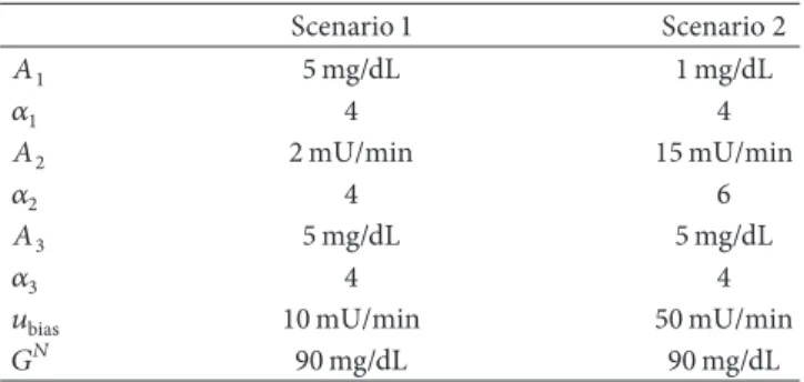
Table 2: The parameters of the applied cost function (10).
Scenario 1 Scenario 2
𝐴1 5mg/dL 1mg/dL
𝛼1 4 4
𝐴2 2mU/min 15mU/min
𝛼2 4 6
𝐴3 5mg/dL 5mg/dL
𝛼3 4 4
𝑢bias 10mU/min 50mU/min
𝐺𝑁 90mg/dL 90mg/dL
The optimization framework was built up by using the
“Visual Basic” packages of the software “MS EXCEL 2016”
under “Windows 10” operating system. The functional dependencies have been constructed in Visual Basic, and the grid points, parameters, and so forth have been defined on dedicated Worksheets—by using these data the Solver can be easily set up.
4. Results
In order to test the realized control framework we inves- tigated two scenarios. In the first scenario 25 g CHO was considered—5 g over 5 minutes in each240th time instant from the60th one.
In the second scenario we considered50g CHO intake 10g over 5 minutes in each 240th time instant from the 60th time instant. In both cases200time horizons have been considered within 10 grid points; thus the total simulated time domain was 2000 minutes. The resolution Δ𝑡 was 1 minute in accordance with the properties of the model.
The applied cost-function parameters (which represent the control parameters in this regard) can be found in Table 2.
It should be noted that we have used permanent reference trajectories in both cases denoted by 𝐺𝑁 = 90mg/dL in (9)–(11).
Therefore, in accordance with the aforementioned details, the goal of the control becomes to keep𝐺𝑁 = 90beside respecting the predefined𝑢bias. In this manner—via the cost function—the deviations from these predefined values have been “punished”; namely, the value of the cost function became higher.
During the examinations we have considered the follow- ing range of blood glucose as “healthy” in accordance with [11]: from 70 to 180 mg/dL.
4.1. Results of Scenario 1. In the following the results of Sce- nario 1 are presented. First, the disturbance signal is shown by Figure 1. The applied—calculated—control signal can be seen in Figure 2. It is clear that the controller is able to administer the insulin in accordance with (9)–(11) where𝑢𝑖 = 𝑢bias+ tanh(V𝑖)is prevailed in the control action.
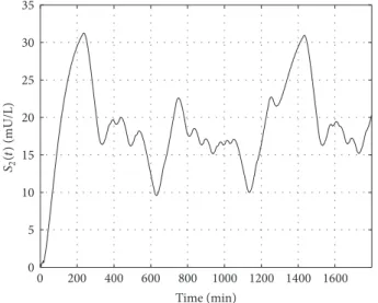
Figures 3 and 4 show the absorption of glucose and its appearance in the blood with the dynamics determined by the model. Figures 5 and 6 show the absorption of insulin from the interstitium and its appearance in blood.
0 0.5 1 1.5 2 2.5 3 3.5 4 4.5 5
0 200 400 600 800 1000 1200 1400 1600 Time (min)
d(t)(g/min)
Figure 1: Applied disturbance (CHO intake)—5g over5minutes at each240th time instant.
The main point can be seen on Figure 7. The controller is able to satisfy the determined conditions and the BG level (𝐺(𝑡)) is inside the predefined range—no hypo- and hyper- glycemia occurred. The BG level approaches the selected reference trajectory (𝐺𝑁) as it is expected.
On Figures 8 and 9 the variation of blood insulin level and the intermediate state variable can be seen.𝑋(𝑡)determines how the blood insulin level affects the blood glucose level, namely, the connection between them.
4.2. Results of Scenario 2. The applied disturbance input in accordance with the detailed protocol can be seen in Fig- ure 10. In this case, we have applied higher inputs in order to be sure that the developed control framework is able to deal with unfavorable external excitation.
Figure 11 reveals the calculated and administered control signal. As it can be seen, its dynamics are significantly different from that of the previous case due to the different settings in the applied cost function.
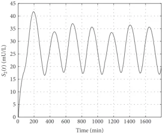
Figures 12 and 13 represent the absorption of the glucose and its appearance in the blood with the dynamics deter- mined by the model. Figures 14 and 15 show the absorption of insulin from the interstitium to the blood.
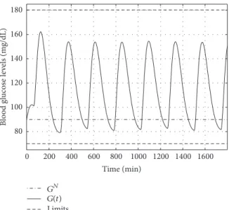
The main result can be seen in Figure 16. Though we have drastically increased the disturbance input signal the controller was able to deal with the situation and realized appropriate control action—without domain violation from the determined𝑢biaspoint of view. The blood glucose level is inside the selected healthy range without any hypo- or hyperglycemia. Moreover, the BG level oscillated around the reference trajectory—𝐺𝑁—as it was expected.
Figures 17 and 18 represent the variation of the blood insulin level and the intermediate state 𝑋(𝑡). Due to the higher frequency of the control signal these are oscillating with a higher frequency as well—which is directly reflected in the blood glucose level as well, since the𝑋(𝑡)mediates the insulin’s effect on𝐺(𝑡).
0 5 10
0 200 400 600 800 1000 1200 1400 1600 Time (min)
u(t)(mU/min)
(a)
0 5 10
0 5 10 15 20 25 30 35 40
Time (min)
Time (min)
u(t)(mU/min)
(b)
Figure 2: Calculated control signals. (a) represents the whole time horizon. (b) shows a piece of the whole time horizon between0and40 minutes.
0 20 40 60 80 100 120 140 160
0 200 400 600 800 1000 1200 1400 1600 Time (min)
D1(t)(mg/dL)
Figure 3: Variation of the first state of the glucose absorption subsystem.
0 10 20 30 40 50 60
0 200 400 600 800 1000 1200 1400 1600 Time (min)
D2(t)(mg/dL)
Figure 4: Variation of the second state of the glucose absorption subsystem.
5. Discussion
In this research our main goal was to design a RHC which is able to control the given patient model and, further, to do that
0 5 10 15 20 25 30 35
0 200 400 600 800 1000 1200 1400 1600 Time (min)
S1(t)(mU/L)
Figure 5: Variation of the first state of the insulin absorption subsystem.
0 5 10 15 20 25 30 35
0 200 400 600 800 1000 1200 1400 1600 Time (min)
S2(t)(mU/L)
Figure 6: Variation of the second state of the insulin absorption subsystem.
by developing such a RHC controller which can be effectively combined with the RFPT principles in our later work by using the detailed NP environment. These goals have been reached.
0 200 400 600 800 1000 1200 1400 1600 Time (min)
GN G(t) Limits 80
100 120 140 160 180
Blood glucose levels (mg/dL)
Figure 7: Variation of the blood glucose level over time.
0 0.002 0.004 0.006 0.008 0.01 0.012
0 200 400 600 800 1000 1200 1400 1600 Time (min)
X(t)(1/min)
Figure 8: Variation of the insulin-excitable tissue glucose uptake activity over time.
0 200 400 600 800 1000 1200 1400 1600 Time (min)
0 0.5 1 1.5 2
I(t)(mU/L)
2.5 3 3.5 4
Figure 9: Variation of the blood insulin level over time.
0 1 2 3 4 5 6 7 8 9 10
0 200 400 600 800 1000 1200 1400 1600 Time (min)
d(t)(g/min)
Figure 10: Applied disturbance (CHO intake)—10g over5minutes at each240th time instant.
In our first scenario we aimed to test the control environ- ment under strict constraints—the collection of them can be found in Table 2. In detail,𝐴1, 𝐴3 = 5mg/dL and𝛼1, 𝛼3 = 4 mean that we punished the deviation of𝐺(𝑡)from𝐺𝑁heavily above5mg/dL during the control action and in the terminal points of the cycles. We applied not just a restriction on the value of𝑢(𝑡)via𝑢bias, but also we penalized the control signals above2mU/min as it is reflected in𝐴2and𝛼2.
In the second scenario we investigated the “robustness”
of the controller by using highly oscillating, unfavorable disturbance input in a cyclic way. As in the previous case, the controller was able to perform well—beside all of the restrictions that have been considered.
The main results can be seen in Figures 7 and 16. It is clearly visible that the main requirement has been satisfied, since the BG level was kept by the controller in the healthy range.
6. Conclusions and Future Work
In this paper we have proposed a possible design scheme for RHC controller by using a NP approach in order to control Type 1 Diabetes Mellitus. We have applied the MS EXCEL’s embedded Solver solution which is based on the Generalized Reduced Gradient method in order to realize the control environment. Two different scenarios have been applied to test our approach—the results have been satisfactory.
In the first scenario we applied “soft” disturbance and smaller penalties via the developed cost function in order to make sure that the controller design is possible and appro- priate control action can be achieved by using the continuous optimization. In the second test scenario we used unfavor- able, cycling disturbance signal with high amplitude to test the “robustness” of the proposed controller. The developed RHC controller was able to handle the load and provided satisfactory control action. Furthermore, in both cases the BG level was kept in the predefined healthy range.
In our future work we are going to extend the developed RHC controller with an additional RFPT framework in order
0 20 40
0 200 400 600 800 1000 1200 1400 1600 Time (min)
u(t)(mU/min)
(a)
0 5 10
u(t)(mU/min)
15 20 25 30 35 40 45 50
Time (min) (b)
Figure 11: Calculated control signals. (a) represents the whole time horizon. (b) shows a piece of the whole time horizon between0and40 minutes.
0 50 100 150 200 250 300
0 200 400 600 800 1000 1200 1400 1600 Time (min)
D1(t)(mg/dL)
Figure 12: Variation of the first state of the glucose absorption subsystem.
0 20 40 60 80 100 120
0 200 400 600 800 1000 1200 1400 1600 Time (min)
D2(t)(mg/dL)
Figure 13: Variation of the second state of the glucose absorption subsystem.
to empower it with adaptive property. We will investigate the solution from robustness, adaptivity, and other aspects’ points of view.
Conflicts of Interest
The authors declare that there are no conflicts of interest regarding the publication of this paper.
0 5 10 15 20 25 30 35 40 45 50 55
0 200 400 600 800 1000 1200 1400 1600 Time (min)
S1(t)(mU/L)
Figure 14: Variation of the first state of the insulin absorption subsystem.
0 5 10 15 20 25 30 35 40 45
0 200 400 600 800 1000 1200 1400 1600 Time (min)
S2(t)(mU/L)
Figure 15: Variation of the second state of the insulin absorption subsystem.
Acknowledgments
Gy. Eigner was supported by the ´UNKP-17-4/I New National Excellence Program of the Ministry of Human Capacities.
The authors would like to acknowledge the support of the
80 100 120 140 160 180
0 200 400 600 800 1000 1200 1400 1600 Time (min)
Blood glucose levels (mg/dL)
GN G(t) Limits
Figure 16: Variation of the blood glucose level over time.
0 0.002 0.004 0.006 0.008 0.01 0.012 0.014 0.016
0 200 400 600 800 1000 1200 1400 1600 Time (min)
X(t)(1/min)
Figure 17: Variation of the insulin-excitable tissue glucose uptake activity over time.
0 200 400 600 800 1000 1200 1400 1600 Time (min)
0 0.5 1 1.5 2 2.5
I(t)(mU/L)
3 3.5 4 4.5 5
Figure 18: Variation of the blood insulin level over time.
Robotics Special College and the Research, Innovation and Service Center of ´Obuda University.
References
[1] J. Bronzino and D. Peterson,The Biomedical Engineering Hand- book, CRC Press, Boca Raton, FL, USA, 4th edition, 2015.
[2] F. Padula, C. Ionescu, N. Latronico, M. Paltenghi, A. Visioli, and G. Vivacqua, “A gain-scheduled PID controller for propofol dosing in anesthesia,”IFAC-PapersOnLine, vol. 28, no. 20, pp.
545–550, 2015.
[3] I. Nas¸cu, A. Krieger, C. M. Ionescu, and E. N. Pistikopoulos,
“Advanced model-based control studies for the induction and maintenance of intravenous anaesthesia,”IEEE Transactions on Biomedical Engineering, vol. 62, no. 3, pp. 832–841, 2015.
[4] J. S´api, D. A. Drexler, and L. Kov´acs, “Potential benefits of discrete-time controller-based treatments over protocol-based cancer therapies,”Acta Polytechnica Hungarica, vol. 14, no. 1, pp.
11–23, 2017.
[5] J. S´api, L. Kov´acs, D. A. Drexler, P. Kocsis, D. Gaj´ari, and Z.
S´api, “Tumor volume estimation and quasi- continuous admin- istration for most effective bevacizumab therapy,”PLoS ONE, vol. 10, no. 11, Article ID e0142190, pp. 1–20, 2015.
[6] R. Zurakowski and A. R. Teel, “A model predictive control based scheduling method for HIV therapy,” Journal of Theoretical Biology, vol. 238, no. 2, pp. 368–382, 2006.
[7] P. Colmegna, R. S. S´anchez-Pe˜na, and R. Gondhalekar, “Linear parameter-varying model to design control laws for an artificial pancreas,”Biomedical Signal Processing and Control, vol. 40, pp.
204–213, 2018.
[8] G. Eigner, J. K. Tar, I. Rudas, and L. Kov´acs, “LPV-based quality interpretations on modeling and control of diabetes,” Acta Polytechnica Hungarica, vol. 13, no. 1, pp. 171–190, 2016.
[9] L. Kov´acs, “Linear parameter varying (LPV) based robust con- trol of type-I diabetes driven for real patient data,”Knowledge- Based Systems, vol. 122, pp. 199–213, 2017.
[10] A. Haidar, “The artificial pancreas: how closed-loop control is revolutionizing diabetes,”IEEE Control Systems Magazine, vol.
36, no. 5, pp. 28–47, 2016.
[11] A. Fony´o and E. Ligeti,Physiology (in Hungarian), Medicina, Budapest, Hungary, 3rd edition, 2008.
[12] V. Adam,Medical Biochemistry (in Hungarian), Medicina Press, Budapest, Hungary, 4th edition, 2006.
[13] World Health Organization,Global Report on Diabetes, WHO Press, Geneva, Switzerland, 2016.
[14] American Diabetes Association, “Diagnosis and classification of diabetes mellitus,”Diabetes Care, vol. 37, supplement 1, pp.
S81–S90, 2014.
[15] World Hearth Organization,Definition and Diagnosis of Dia- betes Mellitus and Intermediate Hyperglycemia: Report of A WHO/IDF Consultation, World Hearth Organization, 2006.
[16] T. Ferenci, A. K¨orner, and L. Kov´acs, “The interrelationship of HbA1c and real-time continuous glucose monitoring in chil- dren with type 1 diabetes,” Diabetes Research and Clinical Practice, vol. 108, no. 1, pp. 38–44, 2015.
[17] T. Ferenci, J. S´api, and L. Kov´acs, “Modelling tumor growth under angiogenesis inhibition with mixed-effects models,”Acta Polytechnica Hungarica, vol. 14, no. 1, pp. 221–234, 2017.
[18] C. Cobelli, E. Renard, and B. Kovatchev, “Artificial pancreas:
Past, present, future,”Diabetes, vol. 60, no. 11, pp. 2672–2682, 2011.
[19] R. Nimri, N. Murray, A. Ochs, J. E. Pinsker, and E. Dassau,
“Closing the Loop,”Diabetes Technology & Therapeutics, vol. 19, no. S1, pp. S-27–S-41, 2017.
[20] J. B. Lee, E. Dassau, D. E. Seborg, and F. J. Doyle, “Model- based personalization scheme of an artificial pancreas for Type 1 diabetes applications,” in Proceedings of the 2013 American Control Conference (ACC), pp. 2911–2916, Washington, DC, USA, June 2013.
[21] F. Doyle, E. Dassau, D. Seborg, and J. Lee, “Model-based per- sonalization scheme of an artificial pancreas for type I dia- betes applications,” 2015, uS Patent App. 14/792,524, https://www .google.com/patents/US20150306314.
[22] J. E. Pinsker, J. B. Lee, and E. Dassau, “Randomized crossover comparison of personalized mpc and pid control algorithms for the artificial pancreas,”Diabetes Care, vol. 39, pp. 1135–1142, 2016.
[23] M. Jouini, S. Dhahri, and A. Sellami, “Design of robust super- twisting algorithm based second-order sliding mode controller for nonlinear systems with both matched and unmatched uncertainty,”Complexity, vol. 2017, Article ID 1972921, 8 pages, 2017.
[24] J. Kuti, P. Galambos, and P. Baranyi, “Minimal volume simplex (MVS) polytopic model generation and manipulation method- ology for TP model transformation,”Asian Journal of Control, vol. 19, no. 1, pp. 289–301, 2017.
[25] L. Kovacs and G. Eigner, “Convex polytopic modeling of diabetes mellitus: A Tensor Product based approach,” inPro- ceedings of the 2016 IEEE International Conference on Systems, Man, and Cybernetics, SMC 2016, pp. 3393–3398, Hungary, October 2016.
[26] L. Kov´acs, C. Maszlag, M. Mezei, and G. Eigner, “Robust nonlinear model predictive control of diabetes mellitus,” in Proceedings of the 15th IEEE International Symposium on Applied Machine Intelligence and Informatics, SAMI 2017, pp. 55–60, Slovakia, January 2017.
[27] V. N. Shah, A. Shoskes, B. Tawfik, and S. K. Garg, “Closed- loop system in the management of diabetes: past, present, and future,”Diabetes Technology & Therapeutics, vol. 16, no. 8, pp.
477–490, 2014.
[28] D. Boiroux, A. K. Duun-Henriksen, S. Schmidt et al., “Adaptive control in an artificial pancreas for people with type 1 diabetes,”
Control Engineering Practice, vol. 58, pp. 332–342, 2017.
[29] N. Moldov´anyi,Model Predictive Control of Crystallisers [PhD Thesis], Department of Process Engineering, University of Pannonia, Veszpr´em, Hungary, 2012.
[30] D. Q. Mayne, J. B. Rawlings, C. V. Rao, and P. O. M. Scokaert,
“Constrained model predictive control: Stability and optimal- ity,”Automatica, vol. 36, no. 6, pp. 789–814, 2000.
[31] N. Muthukumar, S. Srinivasan, K. Ramkumar, K. Kannan, and V. E. Balas, “Adaptive model predictive controller for web transport systems,”Acta Polytechnica Hungarica, vol. 13, no. 3, pp. 181–194, 2016.
[32] M. Messori, G. Paolo Incremona, C. Cobelli, and L. Magni,
“Individualized model predictive control for the artificial pan- creas: In silico evaluation of closed-loop glucose control,”IEEE Control Systems Magazine, vol. 38, no. 1, pp. 86–104, 2018.
[33] L. Gr¨une and J. Pannek,Nonlinear Model Predictive Control, Springer, London, UK, 2011.
[34] J. Richalet, A. Rault, J. L. Testud, and J. Papon, “Model pre- dictive heuristic control: applications to industrial processes,”
Automatica, vol. 14, no. 5, pp. 413–428, 1978.
[35] P. Li, X. Li, and J. Cao, “Input-to-state stability of nonlinear switched systems via lyapunov method involving indefinite derivative,”Complexity, vol. 2018, Article ID 8701219, 8 pages, 2018.
[36] A. Jadbabaie, J. Yu, and J. Hauser, “Receding horizon con- trol of the Caltech ducted fan: A Control Lyapunov Func- tion approach,” inProceedings of the 1999 IEEE International Conference on Control Applications (CCA) and IEEE Interna- tional Symposium on Computer Aided Control System Design (CACSD), pp. 51–56, August 1999.
[37] A. Jadbabaie, J. Yu, and J. Hauser, “Stabilizing receding horizon control of nonlinear systems: A control Lyapunov function approach,” inProceedings of the 1999 American Control Confer- ence (99ACC), pp. 1535–1539, June 1999.
[38] H. Khan, J. K. Tar, I. J. Rudas, and G. Eigner, “Adaptive model predictive control based on fixed point iteration,”WSEAS Transactions on Systems and Control, vol. 12, pp. 347–354, 2017.
[39] H. Khan, A. Szeghegyi, and J. K. Tar, “Fixed point trans- formation-based adaptive optimal control using NLP,” inPro- ceedings of the 2017 IEEE 15th International Symposium on Intelligent Systems and Informatics (SISY), pp. 000237–000242, September 2017.
[40] J. K. Tar, J. F. Bit´o, L. N´adai, and J. A. Tenreiro Machado, “Robust fixed point transformations in adaptive control using local basin of attraction,”Acta Polytechnica Hungarica, vol. 6, no. 1, pp. 21–
38, 2009.
[41] J. Tar, L. N´adai, and I. Rudas,System and Control Theory with Especial Emphasis on Nonlinear Systems, Budapest, Hungary, Typotex, 1st edition, 2012.
[42] S. Banach, “Sur les op´erations dans les ensembles abstraits et leur application aux ´equations int´egrales (About the Operations in the Abstract Sets and Their Application to Integral Equa- tions),”Fundamenta Mathematicae, vol. 3, pp. 133–181, 1922.
[43] F. Chee and T. Fernando,Closed-Loop Control of Blood Glucose, Springer, 2007.
[44] R. Hovorka, V. Canonico, L. J. Chassin et al., “Nonlinear model predictive control of glucose concentration in subjects with type 1 diabetes,”Physiological Measurement, vol. 25, no. 4, pp. 905–
920, 2004.
[45] M. Naerum, “Model predictive control for insulin adminis- tration in people with type 1 diabetes,” Tech. Rep., Technical University of Denmark, 2010.
[46] R. N. Bergman, Y. Z. Ider, C. R. Bowden, and C. Cobelli, “Quan- titative estimation of insulin sensitivity.,”American Journal of Physiology-Endocrinology and Metabolism, vol. 236, no. 6, p.
E667, 1979.
[47] L. S. Lasdon, A. D. Waren, A. Jain, and M. Ratner, “Design and Testing of a Generalized Reduced Gradient Code for Nonlinear Programming,”ACM Transactions on Mathematical Software, vol. 4, no. 1, pp. 34–50, 1978.
[48] D. Fylstra, L. Lasdon, J. Watson, and A. Waren, “Design and use of the Microsoft Excel Solver,”Interfaces, vol. 28, no. 5, pp. 29–
55, 1998.
[49] J. Houston, “Economic optimisation using Excels Solver: A macroeconomic application and some comments regarding its limitations,”Computers in Higher Education Economics Review, vol. 11, no. 1, p. 2, 1997.
[50] A. Ionescu, “Microsoft Office Excel 2010 operational research in Excel 2010,”International Journal of Computer and Information Technology, vol. 2, no. 5, pp. 1026–1064, 2013.
[51] J. Silva and A. Xabadia, “Teaching the two-period consumer choice model with EXCEL-SOLVER,”Australasian Journal of Economics Education, vol. 10, no. 2, pp. 24–38, 2013.
[52] E. Nævdal, “Solving continuous-time optimal-control problems with a spreadsheet,”Journal of Economic Education (JEE), vol.
34, no. 2, pp. 99–122, 2003.
Hindawi
www.hindawi.com Volume 2018
Mathematics
Journal ofHindawi
www.hindawi.com Volume 2018
Mathematical Problems in Engineering Applied Mathematics
Hindawi
www.hindawi.com Volume 2018
Probability and Statistics
Hindawi
www.hindawi.com Volume 2018
Hindawi
www.hindawi.com Volume 2018
Mathematical PhysicsAdvances in
Complex Analysis
Journal ofHindawi
www.hindawi.com Volume 2018
Optimization
Journal ofHindawi
www.hindawi.com Volume 2018
Hindawi
www.hindawi.com Volume 2018
Engineering Mathematics
International Journal of
Hindawi
www.hindawi.com Volume 2018
Operations Research
Journal of
Hindawi
www.hindawi.com Volume 2018
Function Spaces
Abstract and Applied AnalysisHindawi
www.hindawi.com Volume 2018
International Journal of Mathematics and Mathematical Sciences
Hindawi
www.hindawi.com Volume 2018
Hindawi Publishing Corporation
http://www.hindawi.com Volume 2013
Hindawi www.hindawi.com
World Journal
Volume 2018
Hindawi
www.hindawi.com Volume 2018Volume 2018
Numerical Analysis Numerical Analysis Numerical Analysis Numerical Analysis Numerical Analysis Numerical Analysis Numerical Analysis Numerical Analysis Numerical Analysis Numerical Analysis Numerical Analysis
Numerical Analysis
Advances inAdvances in Discrete Dynamics in Nature and SocietyHindawi
www.hindawi.com Volume 2018
Hindawi www.hindawi.com
Differential Equations
International Journal of
Volume 2018 Hindawi
www.hindawi.com Volume 2018
Decision Sciences
Hindawi
www.hindawi.com Volume 2018
Analysis
International Journal of
Hindawi
www.hindawi.com Volume 2018
Stochastic Analysis
International Journal of
![Table 1: The applied parameters of the models in this study [43–45].](https://thumb-eu.123doks.com/thumbv2/9dokorg/1402373.117632/4.900.75.824.132.419/table-applied-parameters-models-study.webp)