PHYSICAL REVIEW A 99, 013413 (2019) Photoelectron holography of atomic targets

(1)

Photoelectron holography of atomic targets

S. Borbély,^1,*A. Tóth,²D. G. Arbó,³K. T˝okési,^2,4and L. Nagy¹

1Faculty of Physics, Babe¸s-Bolyai University, 400084 Cluj-Napoca, Romania

2ELI-ALPS, ELI-HU Nonprofit Ltd., Dugonics tér 13, H-6720 Szeged, Hungary

3Institute for Astronomy and Space Physics IAFE (CONICET-UBA), 1428 Buenos Aires, Argentina

4Institute for Nuclear Research, Hungarian Academy of Sciences (ATOMKI), P.O. Box 51, H-4001 Debrecen, Hungary

(Received 27 September 2018; published 11 January 2019)

We study the spatial interference effects appearing during the ionization of atoms (H, He, Ne, and Ar) by few-cycle laser pulses using single-electronab initiocalculations. The spatial interference is the result of the coherent superposition of the electronic wave packets created during one half cycle of the driving field following different spatial paths. This spatial interference pattern may be interpreted as the hologram of the target atom.

With the help of a wave-function analysis (splitting) technique and approximate (strong-field and Coulomb- Volkov) calculations, we directly show that the hologram is the result of the electronic-wave-packet scattering on the parent ion. On the He target we demonstrate the usefulness of the wave-function splitting technique in the disentanglement of different interference patterns. Further, by performing calculations for the different targets, we show that the pattern of the hologram does not depend on the angular symmetry of the initial state and it is strongly influenced by the atomic species of the target: A deeper bounding potential leads to a denser pattern.

DOI:10.1103/PhysRevA.99.013413

I. INTRODUCTION

When intense and ultrashort laser pulses interact with atoms, depending on the Keldysh parameter, the dominant induced processes are above-threshold, tunneling, or over- the-barrier ionization [1]. The momentum distribution of the continuum electrons produced by such ionization processes is modulated by interference effects, which are created by the superposition of electronic wave packets following different paths [2]. From the possible wave-packet interference scenarios [2], in the present work we focus on the spatial interference and discuss briefly also the temporal interference.

Temporal interference occurs when electronic wave packets emitted at different parts of the driving laser pulse are coherently added, leading to an interference pattern in the momentum distribution of the continuum electrons [3–8]. The structure of the formed interference pattern can be understood in a simple semiclassical picture [2,3,5], where the electronic wave packets with the same asymptotic momentum are considered to be emitted at different time moments. Then, under the combined action of the external laser field and the Coulomb potential of the parent ion, these wave packets follow different paths, accumulating different final phases.

Finally, at the end of the laser field the wave packets are coherently added and, depending on their relative phase, they can amplify or reduce the intensity, leading to a measurable [3,4] interference pattern in the electron spectrum.

In the case of spatial interference, the interference pattern is the result of the coherent superposition of the electronic wave packets emitted at about the same time (i.e., during the same pulse quarter cycle), but following different spatial pathways.

*sandor.borbely@phys.ubbcluj.ro

Along these different paths each wave packet accumulates a different phase, which due to the coherent superposition leads to the formation of a radial fringe structure in the electron spectra [2,5,9–15]. The formation of this pattern can be understood with the help of a simple two-path model [2,9,10], where the radial fringe structure emerges as the result of the interference between the direct (i.e., weakly scattered by the parent ion) and indirect (i.e., strongly scattered) wave packets. The existence of these two distinct wave packets was confirmed by more elaborate classical trajectory Monte Carlo simulations [13] for the ground-state hydrogen target, where it was shown that electrons can reach a continuum state with a well-defined momentum following one of the two distinct types of trajectories: Along the first type of trajectory the electrons returned by the laser field are only weakly scattered by the core (i.e., the minimum distance between the returning electron and the parent ion is larger than 5 a.u.), while along the second type of trajectory the returning electrons are strongly scattered by the core (i.e., the minimum distance between the returning electron and the parent ion is

∼1 a.u.). In this picture, by considering the scattered wave packet as the signal and the direct wave packet as the reference wave, the spatial interference pattern can be interpreted as the holographic mapping (HM) [10,13] of the target atom’s state.

The holographic mapping is closely related to the laser- induced electron diffraction (LIED) [16–20], where the electron wave packets induced by the ultrashort laser pulse are scattered by the parent ion during their quiver motion. From the final electron momentum distribution resulting from this electronic-wave-packet diffraction, both structural [16–19]

and temporal [20] information regarding the target atom or molecule can be extracted using laborious procedures [18].

In contrast to LIED, in HM the scattered electronic wave packet (signal) is coherently added to a reference wave

(2)

packet, and the interference between these two leads to a more structured electron momentum distribution with interference minima and maxima. Since the phase of the scattered wave packet is strongly influenced by the short-range part of the bounding potential encoding the structure of the target atom or molecule, the HM has the potential of becoming a powerful tool to investigate the internal structure of atoms and molecules [14,21–23].

As a result of previous experimental [9–11,14] and our theoretical [13,24,25] investigations, the influence of the laser pulse parameters on the shape of the HM pattern is well understood. The density of the interference pattern (i.e., the number of observable interference minima) is determined by a single parameter z₀, the maximum distance reached by the electronic wave packets before the scattering event. For the same target, the increase ofz₀ achieved via the increase of pulse intensity or wavelength leads to an increase of the HM pattern density. The phase accumulated by the scattered wave packet is strongly influenced by the short-range potential of the target atom. As a consequence, the location of the interference minima in the hologram should also be strongly influenced by this short-range potential (i.e., by the atomic species of the target).

One of the main goals of the present work is to investigate how the atomic species influences the details of the hologram. In order to achieve this goal, we solved the time- dependent Schrödinger equation (TDSE) numerically for different atomic targets interacting with the same few-cycle laser pulse. We will show the results for single ionization of H, He, Ne, and Ar targets. We consider the single-active- electron approximation, where the interaction between the active electron and the residual ion is described by a model central potential [26]. In the investigation of these interference effects the laser pulse parameters are chosen in such a way that only one type of interference (spatial or temporal) can be dominant [2–7,9–11,13]. Even in these ideal situations other types of interference patterns are also present and become entangled with the dominant one. The coherent superposition of different interference patterns makes the interpretation of the experimental electron spectrum cumbersome. In several cases [2,14], the different interference patterns can be identified using semiclassical or approximate models, but most of these models provide only qualitative agreement with the experimental data. In a large number of experiments the measured data can be reproduced best by ab initio models based on the numerical solution of the TDSE, which lacks a detailed explanation of the physics leading to the final results.

In the present paper we provide a solution for these problems by applying a wave-function analysis technique in parallel to the numerical solution of the TDSE. Applying this approach, we are able to disentangle the different interference patterns, which provides valuable information regarding the physics of the processes leading to the formation of the interference patterns.

The present paper is structured as follows. This section is followed by Sec. II(Theory), where our approach for the numerical solution of the TDSE for the H, He, Ne, and Ar targets is presented along with the wave-function analysis tool and the Coulomb-Volkov approximation. SectionIII(Results) is divided into two parts. In Sec. III A we investigate the

TABLE I. Parameters of the model potential [see Eq. (2)] for each target atom. The last column contains the value of the first ionization energies.

Target atomZc a1 a2 a3 a4 a5 a6 Ip

H 1.0 0.000 0.000 0.000 0.000 0.000 0.000 0.500 He 1.0 1.231 0.662 −1.325 1.236−0.231 0.480 0.904 Ne 1.0 8.069 2.148 −3.570 1.986 0.931 0.602 0.793 Ar 1.0 16.039 2.007 −25.543 4.525 0.961 0.443 0.579

physics behind the formation of the HM pattern for the H target using the introduced wave-function analysis technique and the Coulomb-Volkov model. In Sec.III Bwe investigate how the atomic species of the target influences the HM pattern.

SectionIVis dedicated to a summary, the conclusions, and a possible extension of our work. Throughout the present article atomic units are used.

II. THEORY

The results presented here are based on the solution of the TDSE for atoms interacting with a few-cycle XUV laser pulse. The Hamiltonian of this system in the framework of the single-active-electron (SAE) approximation can be written as

Hˆ = pˆ²

2 +V_eff(r)+ r· E(t), (1) where ˆp²/2 is the kinetic energy operator,V_eff(r) is the effective interaction potential between the active electron and the residual ion, andr· E(t) is the interaction potential between the active electron and the external laser field expressed in the length gauge using the dipole approximation. TheV_eff(r) potential for the H target is the pure−1/rCoulomb potential, while for the noble-gas targets (He, Ne, and Ar) the following model potential was used:

V_eff(r)= −Z_c+a₁e⁻â²^r+a₃re⁻â⁴^r+a₅e⁻â⁶^r

r . (2)

The potential parameters corresponding to each considered target are chosen according to Tong and Lin [26] and they are shown in TableIalong with the ionization energiesIp.

The electric component of our two-cycle laser pulse is described by a simple plane wave modulated by a sine-square envelope

E(t )=

εEˆ ₀sin²(^{π t}_τ ) sin(ωt+φ₀) fort ∈(0, τ)

0 otherwise, (3)

where ˆεis the polarization direction of the laser field,ωis the frequency of the carrier wave,φ₀is the carrier-envelope phase, andτ is the pulse duration. As in our previous calculations [13,24], we have used a time-symmetric (cosine-shaped) laser pulse (see Fig.1), which was obtained by choosing the carrier- envelope phase as

φ₀= −ωτ 2 −π

2.

The cosine-shaped pulse ensures that the dominant interference pattern corresponds to the HM [5,13]. Due to the short duration of the laser field (two optical cycles of the

(3)

-E₀ -E₀/2 0 E₀/2

E(t)

0 t₁ T/2 t₂ T t₃ 3T/2 t₄ 2T

Time

C1 C2

C3

C4

C5

FIG. 1. Shape of the two-cycle laser pulse used in the present calculations. HereE0 is the amplitude,T =2π/ωis the period of the carrier wave,t_i stands for the time moments when the electric field is zero, andCiindicates the continuum electron wave packets created during each time interval of the laser field. The pulse duration isτ=2T.

driving field) only one (H and Ar) or at most two (He and Ne) dominant continuum electronic wave packets are created. Consequently, the photoelectron momentum distribution is dominated by a single or at most two HM interference patterns. This allows for a detailed study on how the HM pattern is influenced by the laser pulse parameters and by the bounding potential of the target. In experiments the use of such a short laser pulse with stable carrier-envelope phase is difficult, thus the case of many-cycle laser pulses should also be considered. Based on previous experiments [10–12,14], we expect that the formation of the HM interference pattern sur- vives the multicycle regime. Moreover, since in the multicycle regime the asymmetry between the different half cycles is smaller, the difference between the HM patterns in the wave packets created by each half cycle of the driving laser pulse will also be diminished.

The time evolution is governed by the TDSE i∂

∂t(r, t)=Hˆ(r, t), (4) where (r, t) is the time-dependent wave function. In the present work the numerical solution of Eq. (4) is considered in the framework of the time-dependent close-coupling (TDCC) method along with its approximate solution employing the Coulomb-Volkov model.

A. The TDCC model

In the present TDCC approach the time-dependent wave function is expanded in the basis of spherical harmonics Y_lm(r) as

(r, t)=

lm

Rlm(r, t)

r Y_lm(r), (5)

where Rlm(r, t) are the partial radial wave functions. After substituting this ansatz into Eq. (4) and after projecting the resulting equation onto spherical harmonics, the coupled partial differential equations are obtained for the radial wave

functions i∂

∂tR_lm(r, t)=

lm

T_lmlm+V_lml^CP_m+V_lml^C_m+V_lml^EL_m

×Rlm(r, t), (6) where

Tlmlm= −δllδmm

∂²

∂r² is the kinetic energy matrix element,

V_lml^CPm =δllδmm

l(l+1) r²

is the centrifugal potential energy matrix element, V_lml^C m=δllδmmV_eff(r) is the Coulomb potential matrix element, and

V_lml^ELm =rE(t)

3(2l+1)

4π(2l+1)C_10lm^l^m C_10l0^l⁰

is the electron-laser interaction matrix element, withC being the Clebsch-Gordan coefficient.

For the discretization of the radial wave functions the finite-element discrete-variable representation (FEDVR) method [13,27–29] was employed. In the present FEDVR approach the radial coordinate is divided into finite elements (i.e., segments with variable length), and inside each finite element the radial wave functions R_lm(r, t) are represented on a local polynomial basis built on top of a local grid. The local grid points were chosen to be Gauss-Lobatto quadrature points, which ensured the continuity of the wave functions at the finite-element boundaries.

The wave functions propagate in time [i.e., the close- coupling equations (6) are solved] by using the short iterative Lanczos method [30,31] with adaptive time-step control. Be- fore the time propagation, the wave function is initialized as an eigenstate of the atomic target. For the H and He targets the 1seigenstate, for the Ne target the 2peigenstate, and for the Ar target the 3peigenstates of the SAE Hamiltonian are used to describe the outermost electron of the targets. These eigenstates are obtained by the direct diagonalization of the field-free Hamiltonian on the FEDVR grid, which is later used during the time propagation. In the case of the Ne and Ar targets, after each time propagation step, the time-dependent wave function is orthogonalized to the 1s and 2s states (Ne and Ar) and the 2p and 3s (only Ar) states. In the SAE this orthogonalization prevents the deexcitation of the electron into these states, which are occupied by the inner electrons in the modeled atoms.

Throughout the calculations only linearly polarized laser pulses are used, thus the Hamiltonian [see Eq. (1)] has a cylindrical symmetry around the laser polarization axis ˆε. As a consequence, during the transitions induced by the laser pulse, the magnetic quantum number does not change (m=0).

Since the initial states ψ_i are prepared with m=0, in the partial wave expansion (5) of the wave function only partial waves with m=0 will be populated, which considerably reduces the size of the angular basis. During the numerical convergence tests, we find that converged results are obtained

(4)

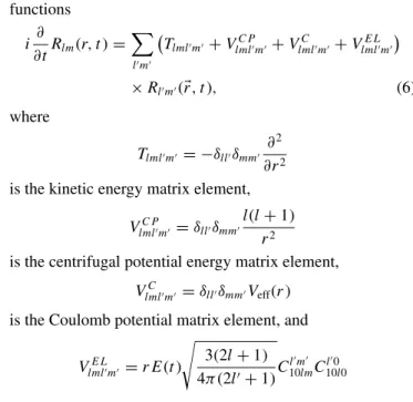
(t=0) (t1) B(t1) B(t2) B(t2) B(t3) B(t3) B(t4) B(t4) B(t= ) B(t= )

C1(t1) C1(t2) C2(t2) C2(t3) C3(t3) C3(t4) C4(t4) C4(t= ) C5(t= )

C1(t2) C1(t3) C2(t3) C2(t4) C3(t4) C3(t= ) C4(t= )

C1(t3) C1(t4) C2(t4) C2(t= ) C3(t= )

C1(t4) C1(t= ) C2(t= )

C1(t= )

FIG. 2. Illustration of the wave splitting technique. Solid red arrow indicate the time propagation and the dotted blue arrows the wave function splitting. HereBis the bound part of the wave function, whileCiare the continuum partial wave functions created during different time intervals of the laser field.

by using the following numerical parameters: angular basis sizel_max=90, radial simulation box sizer_max=100 a.u.with 80 finite elements (i.e., segments with variable length ranging from 0.5 a.u. up to 1.0 a.u.), and nine basis functions in each finite element.

Electron momentum distributions can be calculated as dP

dk = |Tif|², (7) where Tif is the T-matrix element corresponding to the transition ψi →ψf. After the end of the laser pulse Tif is obtained by projecting the time-dependent wave function onto exact continuum eigenstatesψ_f of the field-free Hamiltonian.

These eigenstates are obtained by integrating the radial sta- tionary Schrödinger equation for the given continuum electron energies using the Numerov method [32].

B. Wave-function splitting technique

In the time moments t_k when the r· E(t) interaction term in the Hamiltonian (1) vanishes (these time moments are indicated by vertical dashed lines in Fig. 1), the time- dependent wave function can be split into two parts(r, ti)= B(r, ti)+C(r, ti), where

B(r, t_i)=

nlm

c_nlm(ti)ψnlm(r)

describes the bound part of the wave function [withψnlm(r) being the bound eigenfunctions of the field-free Hamiltonian]

and C(r, ti) the continuum part. In practice, this wave- function splitting can be performed by subtracting from the full wave function the contribution of the bound eigenstates via the Gram-Schmidt orthogonalization algorithm.

In the proposed wave-function splitting technique the studied system propagates in time from the beginning of the laser pulse (t=0) until the first zero point of the electric field (t =t₁). At this moment the wave function splits into the continuum [C1(t₁)] and bound [B(t₁)] partial wave functions.

Then these two partial wave functions independently propagate further in time until the next zero point of the electric field (t=t₂). During the time propagation betweent₁ andt₂ further ionization fromB and electron recapture fromC1

can occur. In order to account for this, from C1 the bound part is extracted and added toBand fromBthe continuum part is extracted and stored att=t₂in a newly created partial wave functionC2. This procedure is continued until the end of the laser pulse, as it is shown in Fig.2. The partial wave functions are independently propagated (indicated by red solid

arrows in Fig.2) between the zero points of the laser field. At each zero point of the laser field (ti) the partial wave functions are rearranged: From the continuum partial wave functions the bound parts are extracted and added to the bound partial wave functionB, and fromBthe continuum part is extracted and stored in a newly created continuum wave packetCi.

As a result of this procedure, at the end of the time propagation (i.e., at the end of the laser pulse) we end up with a partial wave functionBcontaining the bound part of the full wave function and a set of partial wave functionsCi (i∈[1, N], whereN is the number of time intervals in the driving laser field). The continuum partial wave functionCi contains the continuum electron wave packet created during theith time interval of the laser field (i.e., between the ti−1 andti zero points of the electric component witht₀=0 corresponding to the beginning of the pulse andt_N=τ to the end of the pulse).

The momentum distribution of the continuum electrons can be calculated separately for each partial wave function Ci. The interference pattern appearing in these spectra can be clearly identified as spatial interference, since each continuum partial wave function describes electronic wave packets created during the same time interval of the driving laser field. Then the partial wave functions can be gradually summed. The pattern in the electron spectrum obtained from the summation of the wave functions can be identified as temporal interference, since they appeared as the result of coherent superposition of electron wave packets created during different time intervals of the driving laser field.

C. The strong-field approximation and the Coulomb-Volkov model

The time-dependent strong-field approximation (SFA) was developed a long time ago to assess atomic photoionization.

The well-known Keldysh-Faisal-Reiss theory of intense-field processes was developed based on the strong-field approximation [1,33,34], while further modifications take into account the important residual Coulomb interaction in the presence of the field [35]. Alternatively, the SFA can be derived within the time-dependent distorted-wave theory [36], where the transition amplitude in thepostform is expressed as

Tif = −i _+∞

−∞

dt f(t)χ⁻

k (t)|zE(t)|ψi(t) , (8) where ψ_i is the initial atomic state with energy −I_p and χ⁻

k (t) is the final distorted-wave function with momentum k and energy E=k²/2. In Eq. (8) the factor f(t) ac- counts for depletion of the ground state and is chosen as

(5)

f(t)=[1−P_ion(t)]^1/2, whereP_ion(t) is the time-dependent ionization probability calculatedad hoc, i.e., within the TDCC model. Iff(t)=1, as in the vast majority of the bibliography, depletion of the ground state is neglected.

Different distorted-wave approximations result from different choices of the distortion potential to be included in

|χ⁻

k [37]. One of the most used choices of |χ⁻

k is the solution of the HamiltonianHf = ^p₂² +zE(t), corresponding to a free electron in the time-dependent electric field (exit- channel distorted Hamiltonian), with eigenenergyk²/2. These solutions are the Volkov states [38]

χ^(V⁾⁻

k (r, t)= exp [i(k+ A)· r]

(2π)^3/2

×exp

−i _+∞

t

dt[k+ A(t)]²

2 , (9)

where the exponent is the Volkov action and A(t )=

−t

−∞dtE(t ) is the vector potential of the field multiplied by the speed of light. The inclusion of Eq. (9) in Eq. (8) leads to the well-known continuum distorted-wave SFA. Ac- cordingly, the influence of the atomic core potential on the continuum state is neglected and therefore the momentum distribution is a constant of motion after the completion of the laser pulse.

For a symmetric electric field [i.e., E(t)=E(τ −t)], when the depletion of the ground state is neglected [i.e., f(t)=1], it is easy to derive that the final momentum distribution is an even function in the longitudinal momentum [37]

dP(kz)

dk = dP(−kz)

dk , (10)

where we have assumed that the initial state has even parity, i.e.,ψ_i(r)=ψ_i(−r). It is well known that the SFA fails to describe ionization for moderately weak fields as well as the slow electron yield even for strong fields [37,39].

The time-dependent distorted-wave Coulomb-Volkov approximation (CVA) improves this deficiency by combining the atomic eigenstate of the continuumψ⁻

k with the final-channel wave function of Eq. (9). For one-electron atoms, i.e.,V(r)=

−Z_T/rwithZ_T the nucleus charge, it results in the Coulomb- Volkov final state first proposed by Jain and Tzoar [40] and later extensively used for ionization by monochromatic low- intensity lasers [33,34,41–44], i.e.,

χ^(CV⁾⁻

k (r, t)=χ^(V⁾⁻

k (r, t)DC(ZT,k,r), (11) where

DC(ZT,k, r)=N_T⁻(k)₁F₁(−iZ_T/k,1,−ik r−ik· r).

(12) The Coulomb normalization factor N_T⁻(k)=exp(π ZT/2k) (1+iZT/k) coincides with the value of the Coulomb wave function at the origin and₁F₁ denotes the confluent hyperge- ometric function. Inserting Eq. (11) into Eq. (8) leads to the CVA, which can be evaluated in closed form [45,46], except for the depletion factorf(t). In the CVA, the simultaneous interactions of the released electron with the residual ionic core and the external field are considered nonperturbatively,

although only approximately since the Coulomb-Volkov states are not exact continuum states. The forward-backward symmetry of Eq. (10) is inherent to the SFA with no depletion, but is broken in the CVA because of the inclusion of the Coulomb distortion in the exit channel [37,47], even if depletion is neglected [i.e.,f(t)=1].

III. RESULTS

A. Physics behind the holographic mapping

Before the presentation of the results obtained for the noble-gas targets we revisit the interference pattern obtained for the H atom in our previous work [13] and we analyze it using the wave-function splitting technique and the Coulomb- Volkov calculations. In this section we investigate the ionization of the H by the two-cycle laser pulse of Fig. 1with the following parameters: ω=0.4445 a.u.,E₀=1 a.u., and τ =28.26 a.u.

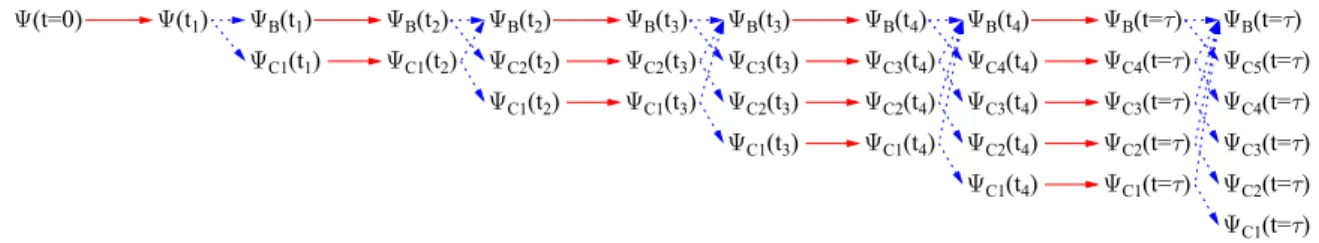
The results of the wave-function splitting technique are summarized in Fig.3, where the distribution of the continuum electrons is presented as a function of momentum components parallel (kpar) and perpendicular (kper) to the laser polarization axis ˆε. The momentum distributions of the continuum wave packets created during each time interval of the driving laser field are presented in Figs. 3(a)–3(e). These wave packets were obtained according to the wave-function splitting technique outlined in Sec.II Band illustrated in Fig.2. It can be seen that only the continuum wave packets created during the second (C2) and third (C3) half cycles of the driving laser field (see Fig.1) have a large norm, thus only these two will have a significant impact on the final momentum distribution of the continuum electrons. This observation is also confirmed by Fig.4, where the total ionization probability (i.e., the norm of the continuum wave packets) is shown as a function of time. The total ionization probability is significantly increased during the second and the third time interval of the driving laser field, i.e., t₁< t < t₃, which means that during these time intervals continuum electron wave packets with a significant norm were created. During the third time interval of the driving field the ionization probability reaches its upper limit of 1, and after that it decreases, indicating electron recapture.

The momentum distribution of the dominant wave packets (C2andC3) shows a characteristic radial interference ridge pattern [see Figs. 3(b) and 3(c)]. Since these interference patterns appear in the continuum wave packets created during the same time interval of the laser field, they can be clearly identified as the result of spatial interference. The interference pattern in wave packet C3 agrees excellently with the interference pattern predicted by the simple two-path model [10,13], since it is scattered by the parent ion only once. In contrast, the interference pattern in the wave packet C2 agrees less with the simple two-path model since it is scattered twice by the parent ion, and a significant portion is recaptured at the end of the laser pulse. As an effect of the multiple scattering of the signal wave, the HM interference pattern is modified at the low electron momentum region, an observation that is in agreement with the SFA [12] and Lippmann-Schwinger equation-based [15] calculations. In the wave packet C1 the interference pattern is smeared out by the multiple scatterings and by the electron recapture. The

(6)

FIG. 3. Distribution of the continuum electrons as a function of the parallel (kpar) and perpendicular (kper) momentum components for a H atom, which interacts with a two-cycle laser pulse [Eq. (3)] with the following parameters:ω=0.4445 a.u.,E0=1 a.u., andτ=28.26 a.u.

(a)–(e) Momentum distributions for the electronic wave packets created during each half cycle of the driving laser field: (a)C1, (b)C2, (c) C3, (d)C4, and (e)C5. (f)–(i) Results of the gradual coherent summation of these wave packets: (f)C1+C2, (g)C1+C2+C3, (h) C1+C2+C3+C4, and (i)C1+C2+C3+C4+C5.

electronic wave packets created during the last two time intervals of the laser pulse (C4 andC5) do not show any trace of interference, which can be explained by the fact that they do not return to the vicinity of the parent ion, thus they are not rescattered.

Figures3(f)–3(i)present the momentum distributions obtained as the result of gradual summation of the electronic wave packets of Figs.3(a)–3(e). After a careful examination

-E₀/2 0 E₀/2

E(t)

0.0 0.25 0.5 0.75 1.0

Ionizationprobability

0 5 10 15 20 25

Time [a.u.]

FIG. 4. Total ionization probability (i.e., the norm of the continuum electronic wave packets) as a function of time. Shown at the top of the figure is the electric component of the driving laser field. The target atom is H and the laser pulse parameters are the same as in Fig.3.

of the results, one can observe that the dominant features present in Fig.3(g)are a simple sum of the features present in the momentum distributions of the dominant wave packets C2 [Fig. 3(b)] and C3 [Fig. 3(c)]. The further addition of wave packets C4 and C5 does not modify significantly the momentum distribution of the continuum electrons [Figs.3(g)–3(i)are nearly identical]. This means that in our case, the temporal interference does not play an important role in the formation of the final momentum distribution of the continuum electrons. This is the direct consequence of the laser pulse shape, which was chosen in such a way to minimize the role of temporal interference. In the momentum distributions of Fig. 3 one can see some spurious circular patterns centered at k_per=0 a.u.andk_par= ±2.18 a.u. (this coincides with the value of the vector potential at the wave- function splitting time momentst₂ andt₃). They appear due to the imperfect separation of the bound and continuum parts of the wave function during the splitting technique. This is strengthened by the fact that they completely disappear after the coherent addition of the partial wave packets.

In Fig. 5, the ab initio results of the TDCC model are compared to the predictions of the SFA and CVA models.

We observed that both approximate models reproduce the main features of the TDCC ionization probability density:

The electrons are predominantly ejected along the laser polarization axis in the forward direction (k_par>0). Beyond this agreement, the interference pattern modulating the ionization probability densities are completely different. In the case of the SFA and CVA models the ionization probability is modulated by interference maxima and minima consisting of quasiparallel arcs, while in the case of the TDCC model

(7)

FIG. 5. Ionization probability density of the H atom as a function of electron momentum components. Calculations were performed in the framework of (a) the strong-field approximation, (b) the Coulomb-Volkov approximation, and (c) the time-dependent close coupling model.

The laser pulse parameters are the same as in Fig.3.

the modulating pattern consists of radial interference maxima and minima. The observed interference pattern in the SFA and CVA is a typical temporal interference pattern [5–7].

Both the SFA and CVA are first-order models, therefore they can describe accurately the ionization, but they do not take into account second-order processes like electron wave-packet rescattering by the parent ion. As a consequence, the ionization probability densities obtained in the framework of the SFA and CVA cannot contain modulations originating from spatial interference (i.e., from the scattering of the returning electronic wave packets by the parent ion). The fact that SFA and CVA completely miss the radial pattern observed in the TDCC results is a good indication that the radial pattern is the result of electronic-wave-packet rescattering on the parent ion.

B. Holographic mapping of noble-gas targets

In order to investigate how the atomic species of the target influences the HM interference pattern, we have performed calculations (besides for H) also for He, Ne, and Ar targets interacting with the same laser pulse with the following parameters: ω=0.4445 a.u., E₀ =1 a.u., and τ =28.26 a.u.,

-2.0 -1.5 -1.0 -0.5 0.0

V

eff

(r) [a.u.]

0.0 0.5 1.0 1.5 2.0 2.5 3.0 3.5 4.0 4.5 5.0

r [a.u.]

H (I_p=0.5) He (I_p=0.904) Ne (I_p=0.793) Ar (I_p=0.579)

FIG. 6. Model potentialVeff(r) as a function of the radial coor- dinaterfor the H, He, Ne, and Ar targets. For each potential curve (thick lines) the ground-state energy of the active electron is shown (thin horizontal lines), while the ionization energyIpfor each target is specified in the legend.

which are identical to the ones used in our previous studies [13]. As it was also shown in Sec. III A, the use of this two-cycle driving pulse ensures that the spatial interference (HM pattern) is dominant. The TDCC calculations were performed in the framework of the SAE approximation, where the interaction between the active electron and the rest of the target atom is modeled by the effective potential given by Eq. (2). Figure6 shows the model potentials for our targets with the respective ionization energies.

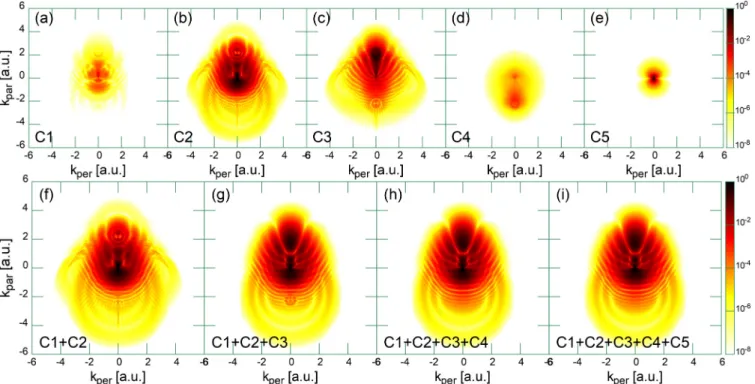
The obtained ionization probability densities as a function of the electron momentum components parallel and perpendicular to the laser polarization axis ˆε are shown in Fig. 7.

At first glance one can observe significant differences among the probability densities, which indicates that the obtained hologram characterizes the target. Upon a deeper look one can observe that the HM patterns for the H and Ar targets and for

FIG. 7. Ionization probability density as a function of electron momentum components parallel and perpendicular to the laser polarization axis. The TDCC results for the H, He, Ne, and Ar targets are compared. The laser pulse parameters are the same as in Fig.3.

(8)

-E0/2 0 E₀/2

E(t)

0.0 0.25 0.5 0.75 1.0

Ionization pr obability

H He Ne Ar

-10 -5 0 5 10 15

<z(t)> [a.u.]

0 5 10 15 20 25

Time [a.u.]

H He Ne Ar (a)

(b)

(c)

FIG. 8. (a) Laser field, (b) total ionization probability, and (c) expectation value of thezcoordinatez(t) as a function of time for the H, He, Ne, and Ar targets. The laser pulse parameters are the same as in Fig.3.

the He and Ne targets are very similar in structure: In the case of the Ar and H atoms the probability density is dominated by a single interference pattern, while in the case of the He and Ne targets the more complex interference pattern is composed of two distinct regions. We have different interference patterns for small and for high electron velocities, and a transition between these two regions is clearly observable at |k| ∼ 1.5 a.u.

In order to investigate the roots of these similarities we have calculated the total ionization probability (i.e., the norm of the wave function’s continuum part) and the expectation value of thezcoordinate according to

z(t) ≡ (r, t)|z|(r, t)

(r, t)|(r, t) . (13) The obtained values as a function of time are presented in Fig.8, where it can be seen that the ionization probability and z(t) curves in the (H,Ar) and (He,Ne) pairs are very similar.

This indicates that the size and the trajectory of the continuum electronic wave packets for the (H,Ar) and (He,Ne) target pairs are also similar. This observation is not surprising, since it is known that in the tunneling and in the over-the-barrier ionization regimes the size of the continuum electronic wave packets is mainly determined by the parameters of the driving laser field and by the ionization energy of the target [48]. In

10^-3 10^-2 10^-1

1 H

Ar

10^-4 10^-3 10^-2 10^-1 1

-60 -30 0 30 60

Electron ejection angle [degree]

He Ne

Normalize d ionization p ro bability d ensity

k=2.6 a.u.

(a)

(b)

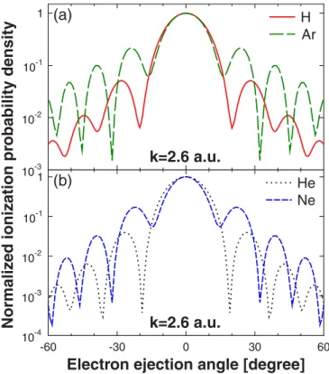
FIG. 9. Angular distribution of the continuum electrons at fixed k=2.6 a.u.electron momentum for different atomic targets: (a) H and Ar and (b) He and Ne. For an easier comparison the angular distributions are normalized. The electron ejection angle is measured from the laser polarization axis. The laser pulse parameters are the same as in Fig.3.

our case the driving laser field is the same, while the ionization energies for the H and Ar targets and for the He and Ne targets are close (see Fig.6or TableI).

The density of the HM interference pattern is determined by the phase difference between the direct and scattered electron trajectories, which is dominantly influenced by the shape and size of the trajectories and by the strength of the scattering potential. In the case of the H and Ar (He and Ne) targets where the electron trajectories are similar (see Fig. 8) the significant quantitative differences between their HM pattern can be attributed to the different scattering potentials. In order to further explore these quantitative differences, the angular distributions of the photoelectrons were calculated. Figure9 shows the angular distribution of the photoelectrons atk= 2.6 a.u. For an easier comparison, the angular distributions are normalized, while the electron ejection angle is measured from the laser polarization axis ˆε.

Deep interference minima were observed for each target, however the location of these minima significantly differs from target to target. Comparing the H and Ar results [see Fig.9(a)], it can be observed that for the Ar target the density of the interference minima is higher (i.e., the distance between the interference minima is smaller) than that of H. This quantitative difference between the H and Ar HM patterns can be explained based on simple physical arguments: Since the trajectories of the continuum electronic wave packets in the presence of the laser field for the H and Ar targets are similar, the root of the observed differences must be sought in

(9)

the phases accumulated by the direct and indirect (scattered) electron paths. We know from our previous classical simulations [13] that during the scattering of the electronic wave packets, the typical minimum distance between the returning electron and the target is about 1 a.u.for the indirect paths and 8 a.u.for the direct paths. For both targets the electron on the direct path experiences the same potential since the bounding potentials for the H and Ar targets are practically the same forr >5 a.u.(see Fig.6). As a consequence, the phase of the direct electronic wave packets (reference phase) are nearly the same in both cases. In contrast, the electron along the indirect (strongly scattered) path experiences a much deeper bounding potential for the Ar target than for H, consequently it has a larger velocity in the vicinity of the target core. A larger velocity along the same path means that the indirect wave packet accumulates a larger phase for the Ar atom compared to the H atom. During the formation of the HM pattern when the interference between the direct and indirect electronic wave packets occurs, a larger phase accumulated by the signal wave (indirect wave packet) translates to a denser interference pattern for the Ar target.

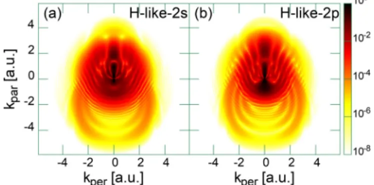
When the H and Ar targets are compared the different angular symmetry of their initial states (s state for H and p state for Ar) should be mentioned. At first glance, the denser HM pattern in the case of the Ar target might be caused by the higher angular momentum of the initial state (i.e., by the higher angular momentum channel reachable for the final state). However, in the following we show that this explanation is not valid. In order to explore the influence of the initial state’s angular momentum on the HM pattern we have performed calculations for the same target with different initial states. In order to ensure similar electron trajectories the ionization energy corresponding to the different initial states should be the same, which can be ensured by choosing as the target a H-like atom, since in this case the ionization energy does not depend on the angular momentum of the initial state.

In the present case the effective charge of the H-like core is set toZ_eff=2.152, which ensures that the ionization energy of the 2s and 2p states (0.579) coincides with the ionization energy of the ground-state Ar.

The momentum distributions of the photoelectrons resulting from the interaction of the H-like target with different initial states and the two-cycle laser pulse used throughout this paper are shown in Fig. 10. It can be observed that the momentum distribution of the photoelectron is strongly influenced by the angular momentum of the initial state.

However, the location of the interference minima in the HM pattern is not influenced by the angular symmetry of the initial state. This can be shown by analyzing the angular distribution of the photoelectrons for a fixed photoelectron momentum in Fig. 11. There it can be clearly observed that the location of the interference minima does not depend on the angular momentum of the initial state.

For the He and Ne targets (see Fig.9) the difference in the location of the interference minima is less pronounced, but the interference pattern for the Ne target is slightly denser than for He, which can be explained by the deeper bounding potential in the case of the Ne target. In thek=2.6 a.u.cut (Fig.9) the density of the interference minima in the case of the H and He targets is similar. This similarity is the result of the balance between the effect of the electron trajectories

FIG. 10. Ionization probability density as a function of electron momentum components parallel and perpendicular to the laser polarization axis. The TDCC results for a H-like target started from the 2s and 2pstates are compared. The effective charge of the H-like core is set toZeff=2.152. The laser pulse parameters are the same as in Fig.3.

and of the scattering potential. In the case of the He target compared to the H target thez₀ parameter is smaller, which decreases the density, while the scattering potential is deeper, which increases the density of the HM pattern.

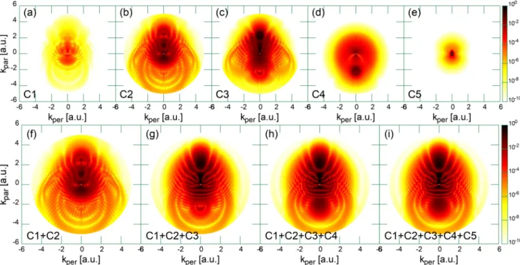
In order to investigate the origin of the qualitative differences between the ionization probability densities obtained for the H and He (Ar and Ne) targets we have performed the wave-function splitting technique for the He target. Figure12 shows the partial momentum distribution of the continuum wave packets created during each half cycle of the driving laser field [Figs.12(a)–12(e)] along with the momentum distribution of the coherently summed wave packets [Figs.12(f)–

12(i)]. According to Fig.12, the wave packets created during the second (C2) and third (C3) time intervals of the laser field are significantly larger than the other partial wave packets. This is also confirmed in Fig.8, where the total ionization probability (i.e., norm of the continuum wave packets) significantly increases during the second and third time intervals.

10^-3 10^-2 10^-1 1

-90 -60 -30 0 30 60 90

Electron ejection angle [degree]

H-like-2s H-like-2p

Ionization pr obability d ensity k=2.2 a.u.

FIG. 11. Angular distribution of the continuum electrons at fixed k=2.2 a.u.electron momentum for H-like targets (2sand 2p). For an easier comparison the angular distributions are normalized. The electron ejection angle is measured from the laser polarization axis.

The laser pulse parameters are the same as in Fig.3.

(10)

FIG. 12. Distribution of the continuum electrons as a function of the parallel (kpar) and perpendicular (kper) momentum components for a He atom interacting with a two-cycle laser pulse with the following parameters:ω=0.4445 a.u.,E0=1 a.u., andτ=28.26 a.u. (a)–(e) Momentum distribution for the electronic wave packets created during each half cycle of the driving laser field: (a)C1, (b)C2, (c)C3, (d)C4, and (e)C5. (f)–(i) Results of the gradual coherent summation of these wave packets: (f)C1+C2, (g)C1+C2+C3, (h) C1+C2+C3+C4, and (i)C1+C2+C3+C4+C5.

As for the case of the H atom, the interference pattern in the momentum distribution of theC3shows good agreement with the prediction of the simple two-path model [10], since theC3wave packet is scattered only once by the parent ion.

In contrast, the interference pattern for the C2 wave packet is modified by multiple scattering on the parent ion.

The final momentum distribution of the continuum electrons is obtained after the coherent summation of the partial wave packets, the two dominant ones being C2 and C3

[see Figs.12(g)–12(i)]. The momentum space center of each partial wave packet can be calculated from their momentum distribution as

k_par Ci = dP dk

Ci

kcos(θk)dk dP dk

Ci

dk

,

(14) where θk is the angle between the polarization axis and the electron momentum vector. Figures12(b)and12(c)show that in momentum space theC2andC3wave packets are shifted compared to each other: The C2 wave packet is centered around k_par _C2= −0.16 a.u., while C3 is centered around k_par _C3=0.49 a.u. As a consequence, the coherent addition of these wave packets does not lead to the appearance of new features. Thus, the small electron momentum region of the final ionization probability density is dominated by the C2

wave packet and the HM pattern associated with it, while the large electron momentum region is dominated by the C3

wave packet. There is a small transitional region between these two domains, where the temporal interference shows up, smearing out the HM patterns. The qualitative difference

between the H and He photoelectron momentum distributions originates from the fact that the H momentum distribution is dominated by the HM pattern of the partial wave packetC2, while the He momentum distribution is a composite of the HM patterns of theC2andC3wave packets.

IV. CONCLUSION AND OUTLOOK

We have studied the ionization of atoms (H, He, Ne, and Ar) by few-cycle laser pulses in the framework of the SAE approximation usingab initio calculations based on the numerical solution of the time-dependent Schrödinger equation.

During the ionization of these targets secondary processes are also present, which can be attributed to the interference between different electronic wave packets. From the various possible interference scenarios we focused our attention on the spatial interference effects, which occur as a result of the coherent superposition of electronic wave packets created during the same half cycle of the driving laser field, resulting in a hologram (HM pattern) of the target atom.

With the help of a wave-packet splitting tool, we have provided evidence that the photoelectron hologram is formed as a result of scattering of the returning electronic wave packets by the parent ion, confirming the conclusions of the simple two-path model [10] and our previous classical simulations [13,24]. Furthermore, we showed that the SFA and CVA ionization probability densities do not contain the HM pattern. Since both of these models omit the scattering of returning electronic wave packets by the parent ion, the absence of the HM pattern in these leads to the conclusion that

(11)

the interference pattern obtained by the TDCC calculation is a hologram, the result of electronic-wave-packet scattering on the residual ion.

We have also investigated the influence of the target atom species on the formation of the HM pattern. We have shown that, for atomic targets with a similar ionization energy (H- Ar and He-Ne), the created continuum wave packets have similar magnitudes and follow similar trajectories in space.

For the case of the H and Ar (He and Ne) targets, despite the similar wave-packet magnitudes and spatial paths followed, the formed HM patterns differ significantly, namely, for the Ar (Ne) target the density of the interference pattern is larger than that of the H (He). The difference in the density of the HM pattern can be attributed to the different potential wells experienced by the scattered electronic wave packets in the vicinity of the target atoms. These observations lead us to the conclusion that the shape of the HM pattern is strongly influenced by the shape of the target’s potential, i.e., by the atomic species of the target. Furthermore, by comparing the momentum distribution of photoelectrons ejected by the H-like target from different initial states (2sand 2p) we showed that, while the momentum distribution is significantly influenced by the angular momentum of the initial state, the density of the HM pattern (which modulates the momentum distribution) is independent of the angular symmetry of the initial state.

In the case of He and Ne targets the obtained ionization probability density contained a complicated interference pattern, with an inner (small electron momentum) and outer (large electron momentum) pattern. With the help of the wave-function splitting technique we were able to disentangle this complex interference pattern, and we have identified

both the inner and outer pattern as the result of the different wave packets scattered by the parent ion. This illustrates the potential of the introduced wave-packet splitting technique in the identification of different interference patterns inab initio simulations.

Since the HM interference pattern is formed as the result of the scattering of the electronic wave packets created independently by each time interval of the driving field, the photoelectron holography has the potential to become a powerful structure analysis tool, with a temporal resolution comparable to the period of the laser field. Due to the present and previous works we have a good understanding of the processes leading to the formation of the HM interference pattern. We know that the photoelectron hologram is sensitive to the short-range potential (i.e., internal structure) of the target atoms. In this sense, the problem of extracting the shape of the target’s short-range potential from HM pattern should be solved. A step forward in solving this inverse scattering problem can be the use of the presented wave-function splitting technique, which in the framework of anab initio calculation gives us information about the form of each wave packet before and after its scattering.

ACKNOWLEDGMENTS

D.G.A. acknowledges Grant No. PICT-2016-2096 of AN- PCyT (Argentina). K.T. and L.N. acknowledge support from the National Research, Development and Innovation Office (NKFIH) Grant No. KH 126886. The numerical calculations were performed using the high performance computing re- sources of Babe¸s-Bolyai University.

[1] L. V. Keldysh, Zh. Eksp. Teor. Fiz.47, 1945 (1964) [Sov. Phys.

JETP20, 1307 (1965)].

[2] X.-B. Bian, Y. Huismans, O. Smirnova, K.-J. Yuan, M. J.

J. Vrakking, and A. D. Bandrauk, Phys. Rev. A 84, 043420 (2011).

[3] F. Lindner, M. G. Schätzel, H. Walther, A. Baltuška, E. Goulielmakis, F. Krausz, D. B. Miloševi´c, D. Bauer, W.

Becker, and G. G. Paulus,Phys. Rev. Lett.95,040401(2005).

[4] R. Gopal, K. Simeonidis, R. Moshammer, T. Ergler, M. Dürr, M. Kurka, K.-U. Kühnel, S. Tschuch, C.-D. Schröter, D. Bauer, J. Ullrich, A. Rudenko, O. Herrwerth, T. Uphues, M. Schultze, E. Goulielmakis, M. Uiberacker, M. Lezius, and M. F. Kling, Phys. Rev. Lett.103,053001(2009).

[5] D. G. Arbó, E. Persson, and J. Burgdörfer,Phys. Rev. A74, 063407(2006).

[6] D. G. Arbó, K. L. Ishikawa, K. Schiessl, E. Persson, and J.

Burgdörfer,Phys. Rev. A81,021403(2010).

[7] D. G. Arbó, K. L. Ishikawa, K. Schiessl, E. Persson, and J.

[8] D. G. Arbó, K. L. Ishikawa, E. Persson, and J. Burgdörfer,Nucl.

Instrum. Methods Phys. Res. Sect. B279,24(2012).

[9] T. Marchenko, Y. Huismans, K. J. Schafer, and M. J. J.

Vrakking,Phys. Rev. A84,053427(2011).

[10] Y. Huismanset al.,Science331,61(2011).

[11] Y. Huismans, A. Gijsbertsen, A. S. Smolkowska, J. H.

Jungmann, A. Rouzée, P. S. W. M. Logman, F. Lépine, C.

Cauchy, S. Zamith, T. Marchenko, J. M. Bakker, G. Berden, B. Redlich, A. F. G. van der Meer, M. Y. Ivanov, T.-M. Yan, D. Bauer, O. Smirnova, and M. J. J. Vrakking,Phys. Rev. Lett.

109,013002(2012).

[12] D. D. Hickstein, P. Ranitovic, S. Witte, X.-M. Tong, Y.

Huismans, P. Arpin, X. Zhou, K. E. Keister, C. W. Hogle, B.

Zhang, C. Ding, P. Johnsson, N. Toshima, M. J. J. Vrakking, M.

M. Murnane, and H. C. Kapteyn,Phys. Rev. Lett.109,073004 (2012).

[13] S. Borbély, A. Tóth, K. T˝okési, and L. Nagy,Phys. Rev. A87, 013405(2013).

[14] G. Porat, G. Alon, S. Rozen, O. Pedatzur, M. Krüger, D.

Azoury, A. Natan, G. Orenstein, B. D. Bruner, M. J. J.

Vrakking, and N. Dudovich,Nat. Commun.9,2805(2018).

[15] H. Agueny and J. P. Hansen, Phys. Rev. A 98, 023414 (2018).

[16] M. Okunishi, T. Morishita, G. Prümper, K. Shimada, C. D. Lin, S. Watanabe, and K. Ueda,Phys. Rev. Lett.100,143001(2008).

[17] S. Micheau, Z. Chen, A. T. Le, J. Rauschenberger, M. F. Kling, and C. D. Lin,Phys. Rev. Lett.102,073001(2009).

[18] J. Xu, Z. Chen, A.-T. Le, and C. D. Lin, Phys. Rev. A82, 033403(2010).

(12)

[19] C. D. Lin, A.-T. Le, Z. Chen, T. Morishita, and R. Lucchese, J. Phys. B 43,122001(2010).

[20] C. I. Blaga, J. Xu, A. D. DiChiara, E. Sistrunk, K. Zhang, P.

Agostini, T. A. Miller, L. F. DiMauro, and C. D. Lin,Nature (London)483,194(2012).

[21] M. Meckel, D. Comtois, D. Zeidler, A. Staudte, D. Pavicic, H. C. Bandulet, H. Pepin, J. C. Kieffer, R. Doerner, D. M.

Villeneuve, and P. B. Corkum,Science320,1478(2008).

[22] X.-B. Bian and A. D. Bandrauk,Phys. Rev. Lett.108,263003 (2012).

[23] M. Meckel, A. Staudte, S. Patchkovskii, D. M. Villeneuve, P.

B. Corkum, R. Doerner, and M. Spanner,Nat. Phys.10,594 (2014).

[24] S. Borbély, A. Tóth, K. T˝okési, and L. Nagy,Phys. Scr.T156, 014066(2013).

[25] A. Tóth, S. Borbély, K. T˝okési, and L. Nagy,Eur. Phys. J. D 68,339(2014).

[26] X. M. Tong and C. D. Lin,J. Phys. B38,2593(2005).

[27] B. I. Schneider and L. A. Collins, J. Non-Cryst. Solids 351, 1551(2005).

[28] J. Feist, S. Nagele, R. Pazourek, E. Persson, B. I. Schneider, L.

A. Collins, and J. Burgdörfer,Phys. Rev. A77,043420(2008).

[29] S. Borbély, J. Feist, K. T˝okési, S. Nagele, L. Nagy, and J.

[30] T. J. Park and J. C. Light,J. Chem. Phys.85,5870(1986).

[31] B. I. Schneider, J. Feist, S. Nagele, R. Pazourek, S. Hu, L.

A. Collins, and J. Burgdörfer, inQuantum Dynamic Imaging, edited by A. D. Bandrauk and M. Ivanov, CRM Series in Mathematical Physics (Springer, New York, 2011).

[32] B. V. Noumerov,Mon. Not. R. Astron. Soc.84,592(1924).

[33] F. H. M. Faisal,J. Phys. B6,L89(1973).

[34] H. R. Reiss,Phys. Rev. A22,1786(1980).

[35] F. H. M. Faisal and G. Schlegel,J. Phys. B38,L223(2005).

[36] D. Dewangan and J. Eichler,Phys. Rep.247,59(1994).

[37] D. G. Arbó, J. E. Miraglia, M. S. Gravielle, K. Schiessl, E. Persson, and J. Burgdörfer, Phys. Rev. A 77, 013401 (2008).

[38] D. M. Volkov,Z. Phys.94,250(1935).

[39] D. G. Arbó, S. Yoshida, E. Persson, K. I. Dimitriou, and J.

Burgdörfer,Phys. Rev. Lett.96,143003(2006).

[40] M. Jain and N. Tzoar,Phys. Rev. A18,538(1978).

[41] S. Basile, F. Trombetta, G. Ferrante, R. Burlon, and C. Leone, Phys. Rev. A37,1050(1988).

[42] D. B. Miloševi´c and F. Ehlotzky, Phys. Rev. A 58, 3124 (1998).