Effect of Upstream ULF Waves on the Energetic Ion Diffusion at the Earth ʼ s Foreshock.
I. Theory and Simulation
Fumiko Otsuka1 , Shuichi Matsukiyo1, Arpad Kis2, Kento Nakanishi1, and Tohru Hada1
1Faculty of Engineering Sciences, Kyushu University, 6-1, Kasuga-Koen, Kasuga, Fukuoka, 816-8580 Japan;otsuka@esst.kyushu-u.ac.jp
2Research Centre for Astronomy and Earth Sciences, Geodetic and Geophysical Institute, 9400 Sopron, Csatkai u. 6-8, Hungary Received 2017 June 17; revised 2017 October 3; accepted 2017 October 16; published 2018 January 30
Abstract
Field-aligned diffusion of energetic ions in the Earth’s foreshock is investigated by using the quasi-linear theory (QLT)and test particle simulation. Non-propagating MHD turbulence in the solar wind rest frame is assumed to be purely transverse with respect to the background field. We use a turbulence model based on a multi-power-law spectrum including an intense peak that corresponds to upstream ULF waves resonantly generated by the field- aligned beam(FAB). The presence of the ULF peak produces a concave shape of the diffusion coefficient when it is plotted versus the ion energy. The QLT including the effect of the ULF wave explains the simulation result well, when the energy density of the turbulent magneticfield is 1% of that of the background magneticfield and the power-law index of the wave spectrum is less than 2. The numerically obtained e-folding distances from 10 to 32 keV ions match with the observational values in the event discussed in the companion paper, which contains an intense ULF peak in the spectra generated by the FAB. Evolution of the power spectrum of the ULF waves when approaching the shock significantly affects the energy dependence of the e-folding distance.
Key words:methods: numerical –plasmas–scattering –turbulence– waves
1. Introduction
A collisionless shock is thought to be an efficient particle accelerator in space. One of the most plausible acceleration models of galactic cosmic rays is the diffusive shock acceleration (DSA) model (Bell 1978; Blandford & Ostriker 1978). In that model, turbulent electromagnetic waves that are present both upstream and downstream of the shock scatter some charged particles back and force across the shock.
Because the turbulent waves are convected by background flows with differentflow speeds upstream and downstream, the particles gain energy through the scattering process. The process occurs stochastically, leading not only to diffusion in momentum space, but also to diffusion in real space. The spatial diffusion has an especially important role in the DSA model. A smaller spatial diffusion coefficient leads to a larger maximum energy attained by the model. This is because that the particles are well-confined near the shock, due to the smaller diffusion, and have a better chance of crossing the shock many times.
Quasi-linear theory (QLT)can provide the spatial diffusion coefficient, or alternatively, mean free path as a function of the wave turbulence spectrum. The spatial diffusion takes place as a result of pitch-angle scattering across 90° in pitch angle.
Mathematically, the spatial diffusion coefficient is calculated by integrating the pitch-angle diffusion coefficient. Jokipii (1966) first developed the QLT in a so-called magnetostatic slab turbulence model. In the slab model non-propagating Alfvén wave, i.e., time stationary and purely transverse fluctuating field with wave vector along the ambient field, is considered. That theory combined with the slab model is often referred to as the Standard QLT. After Jokipii (1966), many authors discussed the validity of the QLT, and developed several theories in various turbulence models, such as a purely two-dimensional model and a composite model of 1D slab and 2D geometries (see Shalchi 2009 for details). The QLT has often assumed a simple power-law spectrum of the wave
turbulence, and has been successfully applied to problems of diffusion and acceleration of cosmic rays in interplanetary and interstellar media. Near the Earth’s foreshock, however, wave spectra have an intense peak rather than a simple power-law (Fairfield1969; Childers & Russell1972; Trattner et al. 1994;
Kis et al.2007,2017).
Quasi-monochromatic waves categorized as terrestrial fore- shock ULF waves with a period of about 30 sec are often observed in the Earth’s foreshock. A number of studies have discussed the characteristics of the foreshock waves and their associated ion populations, such asfield-aligned beams(FABs) and diffuse ions. There are a number of reviews on the physics of foreshock(e.g., Greenstadt et al.1995; Eastwood et al.2005;
Burgess et al.2012; Burgess & Scholer2015). The foreshock ULF waves often lead to a peak in wave spectrum. The quasi- monochromatic 30 s waves are often observed near the foreshock boundary. They are nearly transverse fluctuations, propagating sunward away from the shock, and have intrinsically right-handed polarity in the solar wind frame.
Hence, these ULF waves are identified as waves generated by FAB ions backstreaming away from the shock through resonant mode instability (Gary et al. 1981; Winske &
Leroy 1984). This wave generation mechanism has been confirmed by in situ observations of low-frequency waves and ion distributions detected byClusterspacecraft(Mazelle et al.
2003; Meziane et al.2003; Kis et al.2007). This fact indicates that the FAB ions generate the monochromatic ULF waves. As one moves deeper into the foreshock, the quasi-monochromatic waves steepen into shocklets with whistler-mode wave trains (Hoppe et al.1981). Also, during convection, these waves grow in amplitude into pulsations, termed short large-amplitude magnetic structures(SLAMS) (Lucek et al.2008). According to the changes in waveform, the peak of the ULF power spectrum becomes broader when the spacecraft further approaches the shock (Greenstadt et al. 1995). These ULF waves will efficiently scatter foreshock energetic ions whose parallel velocities are comparable to that of FAB ions.
© 2018. The American Astronomical Society. All rights reserved.
The diffusion of upstream energetic ions is described by the so-called diffusion-convection equation(e.g., Skilling1975). In steady state, the diffusion-convection equation tells us that density of energetic particles increases exponentially when approaching the shock from the upstream side; density reaches its maximum at the shock, then keeps a constant value downstream(e.g., Jokipii1971). Here, the e-folding distance is determined by the balance between upstream spatial diffusion and solar wind convection. This feature was confirmed by a number of in situ observations of Earth’s bow shock. Trattner et al. (1994)showed the result of statistical analysis of about 300 events where the AMPTE/IRM satellite observed fore- shock energetic ions. The analyzed energy range was 10–67 keV e−1. Later, Kis et al. (2004) and Kronberg et al.
(2009) improved a specific event by using multi-spacecraft data. They used data obtained byClustersatellites in the same period when two of the four satellites separate almost along the upstream magnetic field line. Using theClusterdata, one can estimate the parallel spatial gradient of energetic ion density for a single event. Kis et al. (2004) analyzed the data of lower- energy protons from 10 to 32 keV, whereas Kronberg et al.
(2009) analyzed those of higher energy ions from 42 to 123 keV protons and helium.
All these in situ observations showed an exponential profile of upstream energetic ion density, as expected from the classical diffusion-convection theory. Kronberg et al. (2009) demonstrated that the values of e-folding distances obtained by Kis et al. (2004)and Kronberg et al.(2009)lie approximately on the line as a function of ion energy, confirming that these two observations are actually from the same single event.
Further, the e-folding distances estimated by Kis et al.(2004) are ∼0.5–2.8 Re for ∼11–27 keV ions—apparently smaller than the values obtained by Trattner et al. (1994). This fact reveals that the efficient scattering of ions takes place in the event analyzed by Kis et al.(2004). The events analyzed by Kis et al. (2004) and Kronberg et al.(2009)contained an intense ULF peak in the spectra. In the event, the peak frequency was 0.03 Hz in the spacecraft rest frame, and the velocity of FAB ions was about 1600 km s−1 in the plasma rest frame, corresponding to a FAB energy of ∼5 keV in the spacecraft rest frame (which is described in Section 5). Hence, diffuse ions whose energies are higher than 5 keV will be affected by the ULF waves generated by the FAB.
In this paper, we theoretically and numerically investigate the influence of a ULF wave peak in the spectrum of magnetic fluctuations to spatial diffusion of energetic ions. In Section2, we model the spectrum of magnetic fluctuations containing features of ULF waves as a superposition of multi-power-law spectra that have different power-law indices. For the modeled spectrum, the diffusion coefficient of energetic particles is estimated by using quasilinear theory in Section 3 to discuss the qualitative effect of the ULF peak. Test particle simulation is then performed in Section 4 to quantitatively estimate the diffusion coefficient for various parameters. In Section 5, we apply our test particle scheme to the Cluster observation reported in the companion paper (Kis et al. 2017; hereafter referred to as Paper II) for the 2003 February 18th event, to show that the effect of FAB in the scattering of diffuse ions can be significant. We also discuss the relation between the energetic ion diffusion and wave spectral evolution toward the shock. Finally, a summary and our conclusions are given in Section 6.
2. Wave Spectrum Model
We consider a wave spectrum composed ofNsegments with different power-law indices as
å
a= = = g
=
- -
( ) ( ) ∣ ∣ ( )
p k p p, p k k k k , 1
j N
j j j j j
1
1 j
wherep(k)is a dimensionless power spectral density (PSD)of the magnetic field fluctuating in transverse to the background field, andjindicates the index of segment in wavenumber space.
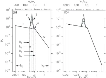
The sum (or integration) of p(k) gives total wave energy,s^2, normalized to the background magneticfield, where a symmetry of the spectrum with respect to k=0 is assumed. Figure 1 shows examples of modeled spectra with N=5. This type of wave spectrum is indeed observed byClustersatellite, as will be shown later in Figure 7. The bottom axis is the normalized wavenumber, kvA W, using the Alfvén speed vA and the ion gyrofrequency Ω. The top axis denotes the corresponding particle parallel velocity, vr/vA, which is calculated from the linear resonance condition-kvr = W, where the wave frequency is omitted by assumingvr?vA. The minimum and maximum wavenumbers are k0= D =k 2pW 6620vA and k5= Wp vA, respectively, and the wavenumber values at the four break points ofp(k)are(k1,k2,k3,k4)=(31, 55, 85, 118)Δk. In the resonant velocity, the break points are represented correspondingly as (v0, v1,v2, v3, v4,v5)=(1054, 34, 19, 12.4, 8.9, π−1)vA. The triangular portion ink1<k<k3corresponds to the ULF peak.
Parameters for the modeled PSD include the power-law index of each segment, γj, total transverse wave energy, s^2(=åp k( )Dk), and the rate of the ULF peak energy to the total one,( (=s^2 -s02) s^2), where σ02 is the wave energy except for the triangular portion in k1<k<k3. In the following, a number of wave models are taken into account.
Their parameters are summarized in Table 1. The PSDs in Figures1(a)and(b)correspond to runs C and D, respectively.
The different triangles in the peak are for different values ofò. In the quasilinear theory and test particle simulations, the PSD is used to give the turbulent magnetic field, with the further assumption that each wave has a random phase. In addition, we assume that the wave electricfield is negligibly small, leading
Figure 1.Modeled wave power spectra for(a)Run C(γ5=1.5)and(b)Run D (γ5=3.0), respectively. Other parameters are written in Table1.
to a static magneticfield turbulence. This is justified when the wave phase velocity, ∼vA, is sufficiently smaller than the velocities of energetic ions to be considered. This turbulence model is the so-called magnetostatic slab model, which is often used as a solar wind turbulence model(e.g., Schlickeiser2002;
Shalchi 2009).
3. Quasilinear Theory
3.1. Spatial Parallel Diffusion Coefficient
We derive a spatial parallel diffusion coefficient with the multi-power-law shape of the wave turbulence spectrum, using the standard quasilinear theory (Jokipii 1971; Schlickeiser 2002; Shalchi2009; Burgess & Scholer2015). In that theory, a pitch angle diffusion coefficient,DmmQL, is given by
p m
= W -
mm ( )∣ ∣ ( )
( )
D k P k
4 1 rB r , 2
QL 2
0 2
where μ is the pitch angle cosine, B0 the ambient magnetic field, kr= -W mv the resonant wavenumber with particle velocity v, and P(k) the transverse wave power spectrum, respectively. Here, P(k) normalized by using B0corresponds to(1). The parallel spatial diffusion coefficient,kQL, is obtained by integratingDmmQL as
ò
k = -m m
- mm
( )
v ( )
D d
8
1 . 3
QL 2
1
1 2 2
QL
Because the segment j of the wave spectrum (Figure 1) contributes tokQLvia correspondingμinterval, the integration of μis divided into Nsegments as
ò
må òmm m
=
- ( )
d d 4
j N 0
1
1 j
j 1
where mj=v vj for v>vj and μj=1 for v<vj, and vj(=Ω/kj) is the resonant velocity at the break points of pk.
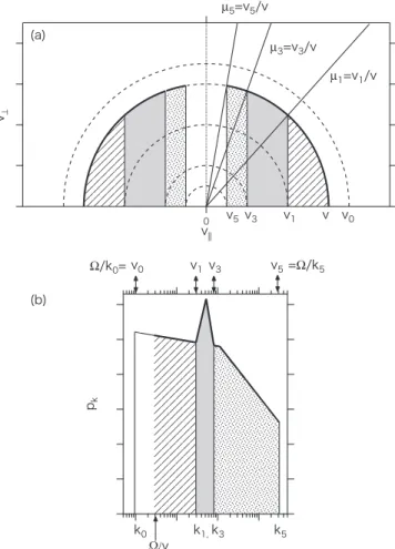
Here, kj>kj−1; then vj<vj−1, equivalently μj<μj−1. The minimum pitch-angle cosine, μN, is finite because pk is truncated at the highest wave number, kN. Figures 2(a) and (b)shows the integration regions in velocity and wavenumber spaces, respectively, for the case ofN=5. Here, the regions corresponding to each other arefilled in the same way. First, let us consider the particles with velocityv1<v<v0. In this case, μ0=1 becausev<v0, otherwiseμj<μj−1<1 forj=2–5.
The particle with the pitch-angle cosine of μ1<μ<μ0
resonates the wave with the wavenumber of Ω/v<k<k1 (shown by the shaded region). Similarly, the particles with μ<μ1 interact with the corresponding resonant waves as shown in Figure2. Thus, in this case, the particles can resonate with the waves in every segments from 1 to 5.
Next, let us consider the particles with the velocity of v2<v<v1. In this case,μ0=μ1=1 because v<v1<v0, otherwise μj<μj−1<1 for j=3–5. Then the integration of thefirst segment vanishes due toμ0=μ1=1, signifying that the particles withv<v1cannot resonate with the waves in the first segment, i.e., k0<k<k1.
Finally, the diffusion coefficientκPQL
in(3)reads
å
k p a
d d
g g
= W
-
- -
g g -
-
( )( ) ( )
B v
2 4 , 5
j N
j
j j
j j
QL 0
2 3
2
max, min,
j j
dmax,j=(4-g mj) j--1g -(2-g mj) j--g, (6a)
2
1
j 4 j
Table 1
Parameters for the Wave Spectrum Used in the Test Particle Simulation
Run g1 g2 g3 g4 g5 s^2a(W^b) %c
A 0.2 −6.8 9.4 0.2 1.5 0.01, 0.1, 1 70
B 0.2 −5.7 8.0 0.2 3.0 0.01, 0.1, 1 70
C1 0.2 0.2 0.2 0.2 1.5 0.2 0
C2 0.2 −3.4 4.9 0.2 1.5 0.29 30
C3 0.2 −5.0 7.1 0.2 1.5 0.40 50
C4 0.2 −6.8 9.4 0.2 1.5 0.67 70
D1 0.2 0.2 0.2 0.2 3.0 0.2 0
D2 0.2 −2.5 3.7 0.2 3.0 0.29 30
D3 0.2 −4.0 5.8 0.2 3.0 0.40 50
D4 0.2 −5.7 8.0 0.2 3.0 0.67 70
E1 0.48 −2.76 4.81 2.45 3.48 0.37(6.98) 71
E2 −0.24 −6.32 6.39 1.90 4.74 0.50(9.49) 37
E3 0.73 −0.84 2.09 2.08 2.08 0.57(13.8) 22
Notes.
aTransverse wave intensity normalized by the backgroundfield.
bTransverse wave intensity in units of10-11erg cc−1.
cRate of the ULF peak intensity.
Figure 2.Schematic picture of resonance regions for the particle with its speed ofvin(a)velocity and(b)wavenumber spaces, respectively. Here, the linear cyclotron resonance condition, kr= -W mv, is assumed. See the text of Section3.1for more detail.
dmin,j=(4 -g mj) j-g -(2 -g mj) j-g. (6b)
2 j 4 j
Whenmj-1=mj=1,δmax,j=δmin,j=2, the contribution ofj th segment vanishes. When γj<2, (5) recovers the standard QLT result as shown in (7).
3.2. Asymptotic Solution
Here, we consider asymptotic solutions of (5) for N=5.
First, let us consider a high-energy particle withv1=v=v0. Here, well-separated k0 and k1 are assumed. In this case, μ0=v0/v=1 otherwiseμj=1. When allγj<2,m02-g1=1 and m2j-gj1. Then dmax,1=2, otherwise dmax,j0 and dmin,j0. Hence, the term ofj=1 only contributeskQL, and the asymptotic solution becomes
k p a g g
W
- -
g- -g
( )( ) ( )
B v
2
2 4 , 7
QL 0
2 1
2 3
1 1
1 1
The above solution is consistent with the standard quasilinear theory (e.g.,(6.64) of Burgess & Scholer 2015). In general a power-law wave spectrum has the steepest slope at dissipation range, i.e., at the highest wavenumber range. Thus, allγj<2 is satisfied ifγ5<2. However, that is not the case with intense peak in the spectrum. In a case such as Figure2(b),γ3>2, and the asymptotic formula(7)fails.
Second, let us consider a low-energy particle with v5<v<v4. In this case, allμj are unity except for μ5<1.
Thus, the terms ofj=1–4 vanish, and the asymptotic solution ofkQL becomes
k pa Wg g g
-g -g - -
- - g-
⎛
⎝
⎜⎜
⎛
⎝⎜ ⎞
⎠⎟
⎞
⎠
⎟⎟
( )( ) ( ) ( )
B v v
v
2 4 2 4 , 8
QL 0
2 5
2 3
5 5
5 5
2
5 5 5
where δmax,5=2 and the largest term of δmin,5 is taken as dmin,5=(4-g m5) 5-g
2 5
. In (8), if v5=v, the last term of the right-hand side (RHS) vanishes for γ5<2. Thus, (8) again recovers the standard QLT without the peak in the spectrum.
However, in our case, μ5=v5/v is not infinitesimally small becausek5isfinite; therefore, the last term is not vanished.
Finally, let us consider the case with γ5>2. In this case, m2j-gjis not less than unity anymore, and the term for the largest pitch-angle, i.e.,m52-g5is the largest term. Thus,δmax,jandδmin,j
have not vanished. The most dominant two terms are
k p a g g
pa g W
- -
+ W
-
g g
g g g
- -
- - -
⎛
⎝⎜ ⎞
⎠⎟
( )( )
( ) ( )
B v
B v v
v 2
2 4
2 . 9
QL 0
2 1
2 3
1 1
0 2 5
2 3
5 5
2
1 1
5 5 5
Whenv1<v<v0, thefirst term arises from the segmentj=1 due toμ0=1, and this term increases withvasv3-g1. On the other hand, the second term arises from the segmentj=5, and this term diverges to infinity if the wave spectrum extends to
¥
k5 , i.e., v5= W k50. This is the so-called 90°
scattering problem. In the standard QLT, the pitch-angle diffusion coefficient becomes Dmm0 form0, represent- ing a free streaming motion of a 90°pitch-angle particle. When γN<2, this free streaming motion does not affect kQL
obtained by integration of κμμ in μ space. This is because kQL is mainly determined by the particles with 0°pitch-angle, as seen in (7) and the first term of the RHS in (8). On the contrary, the spectrum becomes steepened as γN>2, kQL is enhanced due to the free streaming motion of 90°pitch-angle particle, as seen in the second term of the RHS in(9), which shows that the 90°scattering problem causeskQLµv.
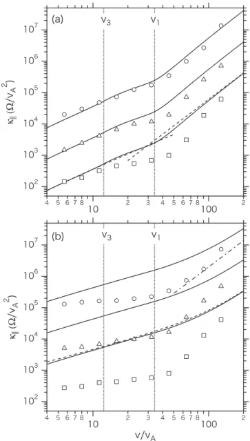
3.3. Comparison between Theory and Simulation Figure3(a)shows the diffusion coefficients obtained by(5) of the QLT and(12)of a test particle simulation, indicated by the solid lines and symbols, respectively. The detail method of the simulation is described in Section4. The parameters used are from Run A in Table1(γ1=0.2 andγ5=1.5). The three lines or data set of symbols correspond to the cases
Figure 3.Diffusion coefficient depending on the transverse wave intensity,s^2, for(a)Run A(γ5=1.5)and(b)Run B(γ5=3), whereγ5is the power-law index of the highest wavenumber regime in the PSD. The solid lines and symbols are obtained by the QLT in(5)and by the simulations in(12), respectively. The results shown by the circles, triangles, and squares are fors^2 =0.01, 0.1and1, respectively. The three dashed lines in(a)and(b)are the asymptotic solutions from(7)to(9). The chained slope in(b)indicates3-g1=2.8.
s^2 =0.01, 0.1, 1from top to bottom, wheres^2 indicates the total transverse wave energy normalized byB02. Both the theory and simulation demonstrate that the diffusion coefficients anti-correlate with s^2 and that the depression of κP appears nearv=v1. Most of the particles that havev=v1can resonate with the waves corresponding to the ULF peak, as shown by the resonance region indicated by the gray region being the largest forv=v1in Figure2(a). Thus, the presence of a ULF wave peak produces a depression that is, equivalently, the concave shape ofk. When the wave energy is small enough (s^2 =0.01), the simulation result is in good agreement with the QLT, as expected. With increasings^2, the result deviates from the theory. In particular, the deviation becomes large at v∼v1. The test particle simulations give a smaller κP and larger concave shape than the QLT. In the figure, the two dashed lines denote the asymptotic QLT solutions (7)and (8) for the higher and lower velocities, respectively, fors^2 =1. These asymptotic solutions match the theoretical solution (5) except forv∼v1. The slope of the asymptotic solution at the higher velocity is ≈3−γ1=2.8, whereas that at the lower velocity is 1.58, which is slightly larger than3 -g5=1.5due to the second term in the parenthesis of (8), i.e., due to the truncation of pkatk5.
Figure3(b)is the same as3(a), butγ5=3.0(Run B). Here, the dashed line denotes the asymptotic solution of (9) for s^2 =1. The difference between the QLT and the simulation is more significant and larger than one order at most. In theory, kQL is proportional to vat v<60vA, and the slope gradually increases for increased v. This gradual change of the slope results from the 90°scattering problem, because the problem causeskQLµv. On the other hand, in the simulation the slope inkclearly changes regardless ofs^2 nearv=v1, and at this velocity the deviation from the QLT becomes the largest again.
If the second term of the RHS in(9)is not considered, the slope in the theory becomes 3−γ1=2.8, indicated by chained line’s slope. Whens^2 =0.01, the slope in the simulation for the higher velocities approaches 2.8. This fact indicates that the discrepancy between the simulation and theory is due to the 90° scattering problem. In other words, the 90°scattering problem in the QLT hides the effect of ULF wave peak onkQL, because the concave shape ofkQL vanishes due to the problem.
In summary, we extended the standard QLT using the multi- power-law wave spectrum to evaluate the spatial parallel diffusion coefficient,k. The extended QLT and the test particle simulations are in good agreement when the power-law index at the highest wavenumber, γ, is less than 2 and the wave energy is low. Otherwise, theκPpredicted by the QLT can be an order of magnitude larger than that obtained by the simulation. This difference is caused by the so-called 90° scattering problem. The standard QLT considers the linear cyclotron resonance, w-k vm = W, where the wave fre- quency, ω, is omitted, and Ω is the proton gyrofrequency.
Accordingly, no particles can satisfy the resonance condition if their pitch angles become 90, leading to Dmm0 and kQL ¥ atμ=0. Of course, including the effect of finite ω in the resonance condition eliminates the singularity at μ=0. However, such waves with ω∼Ωare usually heavily dissipated at high wavenumber range. Also, the effect becomes negligibly small for ion velocities much larger than the Alfvén velocity. Other avenues to solve the problem include nonlinear effects, such as mirroring and the resonance broadening due to
finite amplitude waves (Hada 2003). Even if the wave amplitude is relatively low, the resonance region significantly broadens(see Figure5 of Kuramitsu & Krasnoselskikh2005). Shalchi(2009)has developed second-order QLT, in which the resonance condition, including the effects of finite amplitude waves, is taken into account. They demonstrated that the second-order QLT can explain a parallel mean free path obtained from test particle simulation, despite γ>2 (see Figures6.5 and6.6 of Shalchi 2009). Therefore, it may be worthwhile to apply the second-order QLT to our model, although it is beyond the scope of this paper.
4. Test Particle Simulation
Using the modeled magneticfield spectra shown in Section2, we follow the motions of test particles. Here, we consider the motions of energetic ions in the solar wind rest frame. The so- called one-dimensional slab model is used as our wave turbulence model. In this system, particle energy is conserved because the electricfield is negligible due to the time-stationary field. The wave vectors are parallel and anti-parallel to thex-axis, which is along the ambient magnetic field. The effect of convection by the solar wind will be discussed later.
The following equations are solved for a number of test particles.
= ´
˙ ( )
v v b. 10a
=
˙ ( )
x vx 10b
Here, time and space are normalized to the reciprocal ofΩand vA/Ω, respectively. The magnetic field, b=(1,by,bz), is normalized to the ambient field along the x-axis. Purely transversefluctuatingfields are given by
å
ff
+ = +
+ - +
{ [ ( )]
[ ( )]} ( )
b ib b i kx
i kx exp
exp , 11
y z
k k
k k p
k m ,
,
min max
wherebk= p k( )Dk 2,kmin= D =k 2p L, kmax=π, and system size L=6620. The boundary condition is periodic, phasesfk,pandfk,mare random between 0 and 2π, andp(k)is defined in(1).
Initially, mono-energetic ions with speed v and isotropic pitch angles are uniformly placed in space. Trajectories of ions are calculated by integrating (10). The spatial diffusion coefficient along the xaxis(parallel diffusion)is evaluated as a function of elapsed timescale,τ:
k = áD ñt
x ( )
2 , 12
2
where the bracket denotes the ensemble average of 10,000 ions, and Δx is the ion displacement at the timescale, τ. For a sufficiently long timescale, the diffusion coefficient becomes constant, representing classical diffusion. We perform a number of runs with differentvfor the cases of different wave spectra represented in Table 1. We then obtain the classical diffusion coefficients depending on the velocity, or equiva- lently, on the energy. In each case, we have 10 runs with differentvfrom4 2vA to128vA with a factor of 2 spacing.
4.1. Running Diffusion Coefficient
As an overview, the diffusion coefficients of ions that have
=
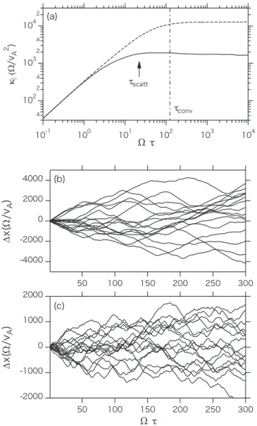
v 32 2vA are plotted in Figure4(a) as a function of τ for Runs C1(ò=0: dashed line)and C4(ò=0.7: solid line). The evolutions of spatial displacement for some particles are shown for Run C1 (Figure 4(b)) and Run C4 (Figure 4(c)) up to Ωτ=300. For both runs, the diffusion coefficients are increasing functions ofτwhenτis small, although they show more or less constant values for large τ. Such a diffusive regime appears over a timescale longer than the pitch angle scattering time, τscatt, shown in Figure 4(a). At this timescale, the change in μ becomes Δμ∼1, representing an isotropic scattering. Trajectories in Figures 4(b) and (c) indicate a Brownian motion along the ambient magnetic field through the isotropic scattering by the turbulent waves at τ>τscatt. The effect of the ULF peak manifests as a diminishing ofκPat large τand also as a shortening ofτscatt. In the following,ks are evaluated on a sufficiently long timescale, Ωτ=104, for variousò(ors^2)andγ5.
4.2. Effect of ULF Peak Wave
Let us see the dependence ofκPon the ULF peak intensity by varyingòfor relatively larges^2 while keeping the spectral part of non-ULF peakfixed. Figure5(a)showsκPobtained for Run C. Here,γ5=1.5. The different markers correspond to different values ofò(=0, 0.3, 0.5, 0.7). Becauses^2 increases withò,κPis smallest for Run C4 (ò=0.7). When the ULF peak exists (ò>0), κP denotes a concave shape similar to what was observed in Figure3. The depression rate,R, is defined as
k k
= =k -
=
( )
R , 13
0 0
and plotted for ò=0.3, 0.5, and 0.7 in Figure 5(b). The maximum depression occurs at a velocity slightly larger thanv1 which is indicated by the vertical line at v=34vA. Here,v1 denotes the maximum parallel velocity with which a particle can resonate with the ULF peak waves. Note that this v1 is apparently larger than the velocity of FAB, i.e.,vw = 19vA. The depression increases withò,leading to the concave shape of κP. However, the maximum depression occurs at the same
~
v v1, regardless of ò. From Figure 2(a), particles that have parallel velocities in the regionv3<v<v1(gray region)can resonate with the waves constituting the ULF peak. Among
Figure 4.Test particle results with an ion speed ofv=32 2vAfor Run C1 (without ULF peak, i.e., ò=0) and C4 (with ULF peak, i.e., ò=0.7). (a)Running diffusion coefficients withò=0 andò=0.7 denoted by dashed and solid lines, respectively. Typical trajectories with (b) ò=0 and (c) ò=0.7, respectively. The vertical chained line in(a)denotes the solar wind convection timescale,τconv(see the text in Section5).
Figure 5. Results for run C (γ5=1.5). (a)Diffusion coefficient, κP, as a function of the ion velocity.(b)Reduced rate,R, ofκPin(13)due to the ULF peak. In(a), the rates of the ULF peak intensity areò=0, 0.3, 0.5, and 0.7, from top to bottom.
these, for the particles havingv<v1, the width of the resonant pitch angle (gray region) increases with increased v. On the other hand, for particles that have v>v1 (stripe region), the width of resonant pitch angle decreases with increased v. This is why the maximum depression occurs atv∼v1.
Figure6is the same as Figure5, but for Run D (γ5=3.0). The basic feature is similar to that of Run C. However, we can confirm that κP is smaller (larger) for larger (smaller) v, compared to Run C. As seen in Figure 1, wave power for k<k4(k>k4)in Run D is higher(lower)than that in Run C.
Therefore, the particles with higher (lower) energy are easier (harder)to scatter.
5. Discussion
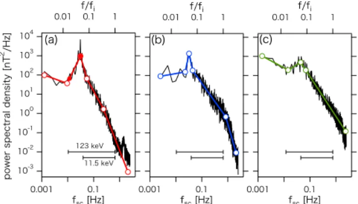
We apply our test particle scheme to understand the diffusion of upstream energetic ions observed by Cluster spacecraft reported in PaperIIfor the 2003 February 18th event. This event contains the high-intensity waves in the foreshock that are produced by the FAB. Figure 7 denotes the transverse wave power spectrum using data in the period of 18:30 UT–21:30 UT;
this period is the main part of the data analyzed in Paper II.
In the panels, from left to right, the spacecraft approaches the bow shock from the upstream side as time elapses:
(a)18:30 UT,(b)21:06 UT, and(c) 21:30 UT, corresponding to distances of (a) 4.5 Re,(b) 1.9 Re, and(c) 1.3 Refrom the shock surface. Here, the distance of the spacecraft from the bow
shock is described in PaperII. The average magnitudes of the magnetic fields are (a) B0=6.5 nT, (b) B0=6.5 nT and (c) B0=7.8 nT, corresponding to ion gyrofrequenciesfi=0.10 Hz and 0.12 Hz, respectively. Other solar wind parameters include plasma density∼3.0 cm−3, solar wind speedvsw∼650 km s−1, the Alfvén speed vA=74 km s−1, the angle between the solar wind velocity and the magnetic field ψ∼147°, the shock normal angleΘBn=20°, and the angle between the solar wind velocity and the shock normal Θsw,n=23°. 1, respectively, as described in Paper II and Kis et al. (2004). The bottom axis indicates the wave frequency in the spacecraft rest frame,fsc. The top axis denotes the wavenumber, k, calculated by using the Doppler shift relation,
p = = y
+ ( )
kv f f
v v
2A 1 cossc , 14
sw A
where f is a wave frequency in the plasma rest frame. We assume a linear dispersion relation of the Alfvén wave propagating along the ambient magneticfield.
It is clear that the wave spectrum is not time-stationary as the spacecraft approaches the shock, which equivalently represents the spatial variation of the wave spectrum. The spectrum clearly contains a peak atfsc∼0.03 Hz, which corresponds to a wave frequency off=−0.05fiin the solar wind rest frame.
In a resonant mode instability, right-handed Alfvén waves, propagating in the same direction as the FAB are generated via cyclotron resonance. The resonance condition gives the resonant frequency in the plasma rest frame as
= - ( )
f v f
v iv , 15
r res
A A
wherevris the resonant parallel velocity. Using(14)and(15), the FAB velocity corresponding to fsc=0.03 Hz becomes vr∼1600 km s−1 in the plasma rest frame, which roughly matches the FAB velocity of 900 km s−1in the spacecraft rest frame observed at ∼8 Re from the shock (Kis et al. 2007). Thus, the observed ULF waves are probably generated by the FAB ions. It can also be seen that the ULF peak is most remarkable at(a). As time elapses, the peak gradually decreases
Figure 6.Same as Figure5, butγ5=3.0(run D).
Figure 7.Power spectral density for the transversal component of the magnetic field observed byCluster 1 at(a)18:30 UT,(b)21:06 UT, and(c)21:30 UT.
Bottom and top axes indicate the wave frequency in the spacecraft rest frame and that in the plasma rest frame normalized by the ion gyrofrequency, respectively. The colored lines indicate the power-lawfitted results in different frequency ranges. Thefitted parameters are shown as run E in Table1. In each panel, upper and lower horizontal bars indicate the resonant frequencies for 123 keV and 11.5 keV ions, respectively. In(a), the solid red circles indicate the lowest and peaked frequencies for the ULF peak.
while the wave energy increases, with a frequency higher than the ULF.
The above three spectra are modeled by the multi-power law spectra, as shown by the colored solid lines in Figure 7. On each line, four break points are indicated by the open circles.
The measured power-law index(γ)of each segment, the wave energy (s^2) normalized by the background field energy, and the rate of the ULF peak energy(ò)are summarized in Table1 as Run E. In that table, the wave energy (W⊥)is displayed in units of erg cc−1. From Run E1 to E3,s^2 orW⊥increase while òdecreases. Note the ratio ofs^2 in run E1 to that in run E3 is different from that ofW⊥, because the backgroundfield energy in Run E3 is 1.3 times larger than that in Run E1.
We numerically evaluate κP by performing additional test particle simulations for Runs E1 to E3. In evaluatingκP, here, care should be taken with the timescaleτ. The simulation frame is the solar wind rest frame where the solar wind velocity is along the background field. Namely, we are looking at the particles scattered along the magneticfield line co-moving with the solar wind. Those particles may start being scattered when the solar wind enters the foreshock region, and they are observed by the spacecraft on a timescale, τconv. To realize the steady-state balance between the diffusion and convection, the particles should be scattered isotropically with the timescale, τscatt, before they are convected by the solar wind over timescaleτconv. Namely,τscatt<τconvshould be satisfied, andκPattains the classical regime atτ=τconv. Figure8shows τconvandτscattas a function of the ion energy. From Figure11 of Kis et al. (2007), the distance from the spacecraft to the foreshock boundary along the magnetic field is Lup≈20 Re, leading to the convection timescale of tconv=Lup vsw,» 200 sin the rough estimate. This corresponds toΩτconv≈120.
The scattering timescale, τscatt, is obtained from numerical simulations as shown in Figure 4 (a). When Esc<42 keV, τscatt<τconv are almost always satisfied; thus, the diffusion concept is valid. On the other hand,τscattforEsc=123 keV is slightly larger thanτconv; this indicates that the particles leave the foreshock and enter the downstream region before being scattered sufficiently. We use classical values ofκPto evaluate the e-folding distance, as assumed in the past studies(Trattner et al. 1994; Kis et al. 2004; Kronberg et al.2009), although
the diffusion approximation is doubtful at 123 keV ions. We discuss this uncertainty later.
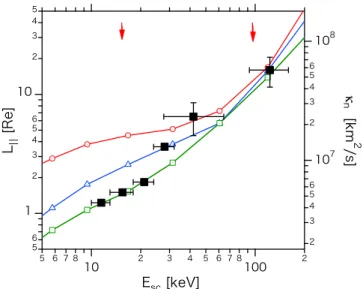
Figure 9 summarizes the numerical results of e-folding distances as compared to the Cluster observations (Paper II;
Kronberg et al. 2009). The numerically obtained values for Runs E1–E3 are plotted, shown by the colored markers, versus the ion kinetic energy in the spacecraft rest frame. In thefigure, observationally obtained values are superimposed by the solid squares. The four solid squares from the lowest energy and two solid squares from the highest energy indicate the values estimated by PaperIIand Kronberg et al.(2009), respectively.
Note that the data from Paper II shown here are slightly modified from those of Kis et al.(2004).
In the diffusion-convection equation in the normal incident frame, the balance between the diffusion and convection terms yields Ln=κn/vsw,n, where Ln=LcosQBn the e-folding distance, vsw,n=vsw cosΘsw,n the solar wind velocity, and kn=kcosQ2Bn the diffusion coefficient. The subscript “n” denotes the direction normal to the shock surface. Next, the e-folding distance along the background field, LP, is numeri- cally estimated by
k
= ( )
L vsw,; 16
where vsw,=vswcosQsw,n cosQBn is solar wind velocity in the de Hoffmann–Teller frame where a motional electricfield vanishes across a shock(e.g., Sections2.5 and6.3 of Burgess
& Scholer 2015). The particle energy in the spacecraft rest frame is then written asEsc=m vp( 2+v ) 2
sw,2 , wherevis the particle speed in the simulation frame and mp is the proton mass. Here, an isotropic velocity distribution of ions in the solar wind frame is assumed.
Runs E1, E2, and E3 correspond to the red circles, blue triangles, and green squares, respectively. These simulation values are close to each other when Esc increases, and the
Figure 8. Typical timescales vs. particle energy. Pitch-angle scattering timescale isτscatt, convection timescale of the solar wind in the foreshock is τconv, and escape timescales far upstream along thefield and from the shock
across thefield areτesc,Pandτesc,⊥, respectively. See the text for definitions. Figure 9. Comparison of e-folding distances between simulation and observations. Bottom axis indicates the ion kinetic energy in the spacecraft rest frame. Left and right axes indicate the e-folding distance along the ambient field (LP)and parallel spatial diffusion coefficient(κn)normal to the shock surface, respectively. Solid squares are the observed values reported in PaperII (four points at low energies)and Kronberg et al.(2009) (two points at high energies). Red circles, blue triangles, and green squares are the simulation results for runs E1, E2, and E3, respectively. Two arrows indicate the energies of 0°pitch-angle particles resonant with the waves that have frequencies shown by the red solid circles in Figure7(a).
observed value for Esc=123 keV matches the simulation result. For Esc<42 keV, the observed LP with the lower energy matches the simulated LP with the PSD closer to the shock. This indicates that the energy dependence of LP is closely affected by the spatial variation of the wave spectrum.
Let us now discuss each of these runs in more detail. The red arrows indicate the energies of 0°pitch-angle particles resonant with the lowest and peaked frequency in the ULF peak, shown by the red solid circles in Figure 7(a). In the energy range between the two arrows, the values of Run E1 are depressed due to the presence of the intense ULF peak (i.e.,ò=71%). The observedLPat 42 keV matches with the depressed LP. In addition, the resonant frequency range for 123 keV is indicated by longer, horizontal bars in Figure 7. The range is obtained from (14) and (15). The minimum resonance frequency corresponds to a 0° pitch-angle of the 123 keV ion, while the maximum one is simplyfixed asfres=−fi, corresponding to a 88°pitch-angle of the 123 keV ion, due to the negligible wave energy for the higher-frequency part. It can be seen that the resonance range fully covers the intense ULF peak. Hence, the particles with 42 and 123 keV may be efficiently and directly scattered by the ULF peak waves.
On the other hand, the observed values for relatively low energies (<21 keV)are in good agreement with run E3 using the PSD(Figure7(c))in the vicinity of the shock. The resonant frequency range for 11.5 keV is indicated by shorter, horizontal bars in Figure 7, the same as in the case for 123 keV. The minimum resonance frequency corresponds to a 84° pitch- angle of the 11.5 keV ion. This frequency range corresponds to segment 4 in the spectrum. In this range, the resonant wave energy increases from (a)1.85×10⁻¹¹ erg cc−1to(c)7.5×
10−11 erg cc−1, and the rate of the resonant wave energy against s^2 increases from (a) 26% to (c) 54%. This fact is approximately equivalent to a hardening of the spectrum, i.e., decreased γ4, toward the shock, while the ULF peak rate, ò, decreases. This implies that the intense ULF wave energy transfers to a frequency higher than the ULF peak, which may result in the smaller e-folding distances at Esc<21 keV.
In summary, we used three different ULF wave spectra observed at different positions from the shock, and demon- strated that the spatial dependence of the wave spectrum significantly affects the e-folding distance of the diffuse ions.
Kronberg et al. (2009) found that the e-folding distance of high-energy ions increases approximately linearly from lower energies as energy per charge is increased, whereas our result show a deviation from this linear dependence on the energy.
Our result suggests that the spatial diffusion of the foreshock energetic ions does not obey the simple picture that the standard QLT predicts, and that the spatial or temporal variation of the wave spectrum should be taken into account.
In our calculation to evaluate the diffusion coefficient as a function of time, we assumed that the wave spectrum does not change along the magnetic field. To include the spectral variation in more detail, particles should experience the evolving foreshock ULF waves as they travel toward the shock during the convection.
The sequence of the wave spectra detected by the spacecraft shows not only a gradual change but also some small variations in time. We carefully chose the time intervals in which the observed spectra explain the observed e-folding distances well, and obtained good agreement with the simulation and observations (Figure 9). We emphasize here that the wave
spectrum far upstream (>2 Re from the shock) never reproduces the small e-folding distance for the diffuse ions with their energies <21 keV. This implies that the small e-folding distances at the lower energy range are caused by the developed ULF power spectrum near the shock, although their association with the shocklet and SLAMS are not clear. Our modeled waveforms are different from these structures due to the random phase approximation.
In our model, we have assumed a balance between convection and diffusion in a steady state. This would be appropriate for the kind of infinite planar shock acceleration described by Bell (1978) and Blandford & Ostriker (1978). However, the Earth’s bow shock has a large curvature, so the process might be modified from a simple DSA model assuming one spatial dimension. Early ISEE spacecraft observations demonstrated that the particles far upstream of the Earth’s bow shock move essentially scatter-free from the shock (Scholer et al.1980). This indicates that the wave activity is not enough to scatter the particles, and that the diffusion concept breaks down far upstream. Terasawa(1981) modifies the ideal DSA model by introducing the scatter-free effect in the terrestrial bow shock. Eichler(1981)also theoretically discussed an effect of particle escape from the shock acceleration region. We now discuss the applicability of the ideal DSA to our model.
Terasawa (1981) introduced a dimensionless parameter, zºvsw,Lup k=Lup L, to characterize the effect of escape far upstream along the magnetic field. Beyond the distance, Lup, from the shock in the upstream region, the particles escape freely due to the absence of turbulent magnetic field. When ζ<1 (weak scattering), particle escape becomes significant, and the diffusion concept may break. In our case,ζ∼16 for 11.5 keV, whereas ζ∼1.3 for 123 keV. This implies that the scattering at 123 keV is not sufficient to allow us to neglect the escape effect, and that the acceleration must be terminated somewhere around this energy.
Typical timescale to escape far upstream is written as tesc,=Lup2 k=ztconv, where tconv=Lup vsw,. Also, a typical timescale to escape across the magneticfield from the shock region is approximated as tesc,^=a2 k^, where a(=6×10⁴km)is the radius of curvature of the bow shock, and k^ is the cross-field diffusion coefficient. The diffusion coefficient is determined from the result obtained by the test particle simulation using a non-compressional two-dimensional turbulence model(Otsuka & Hada2009). From the above, the diffusion coefficient is written ask^~rvK2forK<1, where the dimensionless parameter K=bL^ r, and the wave amplitude b=s^. Here, the wave amplitude, σ⊥, from Table 1 is used, and a perpendicular scale length of the turbulence is roughly assumed to beL⊥;1000 km from the foreshock wave observations (Narita & Glassmeier 2010). In the present study, K<1 throughout the energy range from 11.5 to 123 keV. Accordingly,tesc,^W ~(a L2 ^2) b2.
In Figure8, the escape timescales are plotted as a function of the particle energy,Esc. First,tesc,^is at least 8000 seconds— much larger thanτconv. Hence, the escape due to the cross-field diffusion is negligible, and the particles are almost tied to the field lines during the convection. Second, τesc,Pdecreases for increasedEscand drops belowτscattatEsc=123 keV. This implies that the effect of escape far upstream is not negligible, and the isotropic velocity distribution is not guaranteed.
On the contrary, our simulation assumed a balance between convection and diffusion, which leads to the isotropic velocity