I N HOT STRIP M I L L S
W . A S K
Svenska AB Philips, Stockholm, Sweden
In this paper a new method of measuring the width of hot steel strips to an accuracy of about 0.05 per cent under severe ambient conditions will be described. A short review of other well-known methods will be given before the new method is discussed.
V A R I O U S M E T H O D S
The determination of the position of the opposite edges of an object in space and of their distance from each other can be effected by referring each edge to a fixed plane or line in space. Another way is to use an absolute measuring unit, which follows the movements of the object. A familiar example of the latter method is the sliding caliper. In non-contact measuring methods, e.g. optical methods, many solutions are based on a method of fixed references. But if the only thing that interests us is the distance between the edges, i.e. the width of the object, it is clear that the data on its position in space are superfluous. These data comprise the measuring of two widths at each edge, adding these and subtracting their sum from a fixed width.
Lateral movement of the object is in theory cancelled out by this method, but because two different measuring appliances are used there will always be a certain error in cancellation.
Another method where these fixed references also exist but are not directly used is the method of scanning the whole picture of the measured object by a technique similar to that of television. Apart from discrepancies due to non-linearity in the scanning operation, the accuracy of this method is also proportional to the scanning speed, i.e. lateral movement in the same direction as the scanning motion will give high values for the width, while the other direction will give low values.
The most promising methods for high accuracies are those of the caliper type already mentioned. The central idea here is to evolve a measuring tool which follows the centre line of the object during lateral movement i.e. a fixed position relative to the position of the object. The mechanical, servo-controlled solutions that are now in use are based upon optical
Fig. 1.—3-Mirror, "liminal slit" method.
measurements taken at both edges. Subtraction of these values from each other will instruct the servoloop to follow the object. Allowance for lateral movement of the edges can also be effected by having separate servo-systems to follow the position of the two edges.
The method to be described in detail later in this paper, which coincides in part with that used by another investigator, is based upon a light-inversion principle, one edge being projected to form a virtual image which constitutes
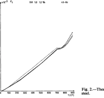
Fig. 2.—Thermal expansion of carbon steel.
a reference edge immediately outside the other, true edge. A simple com- parison is that the caliper consists of the light paths themselves, and is thus totally free from inertia. This "light caliper" can have a fixed total gap greater than the greatest width to be measured, thus giving the width variation as a function of the width of the light issuing from the slit. Another way (Fig. 1) is to use a variable gap which is just barely kept in contact with the two edges of the object. In practice, this method of maintaining a constant minimal gap, which we may call the "liminal-slit" system, employs a closed servo-loop system with the following sequence: liminal-slit light- photocell-amplifier-positioning organ including the gap-defining optics- object-liminal slit. In the closed system it is quite clear that the independent variable (object width) will be followed lineally by the gap-defining optics, disturbed only by variations in the total gain in the chain and the dynamic behaviour of the loop. A s in most balance methods, the static accuracy can be made very high by having high gain in the detection circuit if we are working with an open loop. If we close the loop, the lag of the servo-system impairs the overall accuracy, the net result being determined only by the loop characteristics, which are of course limited by the necessity to avoid self-oscillation.
D E T A I L P R O B L E M S
The phenomena associated with the passage of light through a small slit were investigated long ago. Parallel monochromatic light shows the well- known diffraction fringes, which in this problem are only of interest when they arise from one of the edges (the virtual edge). Using polychromatic light, which we normally do to begin with, entails the spreading and over- lapping of this diffraction effect, resulting in a continuous steady increase in the light intensity from the dark to the bright region. The pure ramp function, which would hold if there were no diffraction and if a point source of light existed, is replaced by a light-flux characteristic beginning with derivate zero and reaching a constant value proportional to the light inten- sity and slit length. The half-shadow and the nearby rectilinear regions are those where the set-point for the servo action is chosen. If we go too near the completely black region, we diminish the "light gain" (change in flux/
change in object width) too much, although on the other hand there will be a lower level of light aberration. This latter is easily seen if we choose a rather big slit (compare the method using a constant total gap, referred to above, in which variations in light intensity will upset the original measured variable).
Another light influence, common to most photoelectric systems, is the bending of light rays in air which is not at a uniform temperature. This is
particularly pronounced if the object has a very high temperature, which is in fact the case with strips in hot rolling mills. The regions which are most active in this respect are those in the vicinity of the edges where the tempera- ture gradient is very high, but the air in the rest of the light path between object and light-receiving components will also have a disturbing effect on the image. The affected regions can be kept in an acceptably steady state by forced air, and a calibration of the variation in width as a function of air velocity indicates what type of blower is necessary for a given accuracy.
A s in other photoelectric applications, interference from extraneous light is easily avoided by using modulated light and/or light of a narrow wave- length band together with selective light filters. If modulation is used, the frequency must be chosen with due regard to the stipulated standards of promptitude in the servo response.
The servo-system, based on A . C . or D.C. methods, must work as sym- metrically as possible, which, when applied to the above-mentioned modified ramp function, is only possible in one of three ways:
7. By using a very narrow working band, so that a part of the curved section can be regarded as a straight line.
2. By putting the set-point sufficiently high up on the straight portion of the flux curve.
3. By using a non-linear servo or a two-step servo with compensated gain.
Which of these methods should be chosen depends on numerous factors, too involved to be explained briefly. However, one point of interest in the servo application of this problem is how to displace the servo signal so as to obtain a plus-minus action. If unmodulated light is used, the photocell signal from the set-point on the flux curve can be balanced either by a bias, supplied from a simple D.C. source, or by a voltage from a similar photocell illuminated by the same light source. Even if the above method is in practice a "zero-light" method, some small quantity must always be available at the set-point. This means, even if this consideration is of a secondary order, that the method employing a second reference cell introduces some degree of counterbalance for light variations in the source. These considerations lead to a very simple solution when using modulated light, that of letting the light chopper alternately intercept two different light paths, one being the normal measuring light path, the other following approximately the same route but travelling outside the object shadow areas. A t the end of their travel, both rays are collected by a lens to one and the same photocell.
The flux at the set-point is then the same from both the rays and gives no A . C . signal to the amplifier. When the width of the measured object varies, the resulting A . C . signal will then automatically discriminate by phase- shift between plus and minus deviation, and can be directly fed to the servo- motor.
One central problem, which has nothing to do with the measured visual width, is the thermal expansion of the object to be measured. Knowledge of the hot width has no practical value, since only after making an expansion correction to yield a value for the cold width can the rolling-mill specialist use it for process control or sorting. T w o factors must be known with the same accuracy, the temperature and the coefficient of expansion, the second being also a function of the first (see Fig. 2). If the temperature interval is small, this function can be taken as linear, and quite a simple correction network can be added to the output signal from the optical gauge. Even if different alloys have different coefficients and the figures are not yet as accurately known as we should like, this problem seems to be of a secondary order. Its influence on the overall accuracy can easily be calculated, and can thus be applied to shed light on the current degree of accuracy in temperature measurement and evaluation of the coefficients and that degree which will in practice be required. Whether sampling or continuous correction will have to be used depends on the range of temperature variation.
C O N S T R U C T I O N
The experimental model was constructed for a width range of 80-450 mm.
The only real reason for its division into two halves was to keep open the possibility of measuring very broad strips outside the above range. For example, in measuring widths of the order of 2000-4000 mm, a U-shaped pattern would not be practical, although the experimental model also has a drawback in the shape of the long intercoupling light ray. In future, there- fore, such large widths will probably be handled by the method mentioned earlier, using one apparatus at each edge and measuring the distance of these edges from a fixed datum edge. In this case, too, the "liminal-slit"
method can be used to achieve measurement accuracy, the width measured in this instance being that of a slit. It is possible to do this with the same construction as that described above. The only difference is that the bright areas are now dark and vice versa, i.e. we have an inverted liminal-slit method. In the same way as before, the difference between a fixed value and the sum of the widths from the two slits gives the wanted width.
The above discussion on the question of measuring range is closely bound up with the freedom of the measured object to move laterally. If we define lateral movement in the form of a percentage figure (total movement/
object width) it is familiar in practice that the figuie decreases with in- creasing width. In the lowest measuring ranges, for example in measuring the diameter of cold-drawn wire, it is quite certain that at many points on the line it will often exceed 100 per cent. However, if we take 100 per cent as
our lower limit, the measurement of wire down to a few millimetres in dia- meter is possible. The optical limitation of the liminal-slit method is about
100 per cent side variation, meaning that the optical right-angle deflecting units are close to each other. Such units can preferably for small dimensions consist of two prisms, one pentagon and one 45°-90°. For this set-up, the maximum lateral movement is 100 per cent.
In the experimental model, lateral movement was determined as an absolute figure, + 30 mm, meaning a maximum side variation of 75 per cent at the lower end of the range down to 13.6 per cent at the upper end.
This follows from the means of adjusting the coarse setting by screwing the units away from each other. (The servo action is perpendicular to this direction.) If we maintain 100 per cent lateral movement over a complete measuring range, coarse setting must therefore be effected in a direction perpendicular to the width to be measured. Theoretically, the latter method of coarse setting allows for a very wide measuring range (infinite!), but in practice it will probably never be raised to more than 10:1. This is due partly to practical limitations and partly to the fact that the length of the light path from the first edge to the second will not decrease in proportion to the width of the object. The half-shadow region, owing in part to dif- fraction phenomena, will therefore be relatively more pronounced at the lower end of the range.
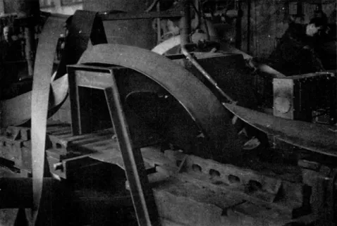
In this connection, too, the possible height variation of the object is of interest, since it determines the outer dimensions of the gauge. If we use a parallel-light gauge method it is as clear as with a caliper gauge that there are no limitations in principle to the height variation. However, if the edge- to-edge light paths are very long, the problems associated with the broadening of the half-shadow region, air temperature influences, etc., will grow in complexity. The first-mentioned, in particular, will change the set-point if it falls within this region. It is possible to avoid these limitations on the height variation in the gap by using a four-mirror instead of a three-mirror light caliper, resulting in a constant edge-to-edge path. (In the three-mirror system, the incoming and outgoing light rays travel in opposite directions, while systems with four mirrors, or any other even number, exhibit the same direction of light travel.) However, this is no real problem in practice, since it is easy to compensate for this effect by adjusting the reflecting units to give a slight deviation from parallelism. Even if there is plenty of scope for lateral and vertical movement of the object, it will readily be understood that this is not sufficient to save such an apparatus when the hot strip gets out of hand and goes its own way among the rolling stands (see Fig. 3), which seems to happen now and then even in the best-regulated mills. T o cope with this problem, and also with the upturned leading and trailing ends of the strip, a special cover with a height guide must be installed. Blowing
Fig. 3.—A strip gone wild.
the surface clean from water and clouds of iron oxide also helps to prevent the distortion in the light path. The method of using very small quantities of light cannot completely counteract these interfering factors, but seems to be very promising in this particular respect. Experience as yet, however, is too short for us to be able to say how large this influence is.
In future installations, the gauge will look like the arrangement shown in Fig. 4. The U-shaped cover can easily be withdrawn from its position in the path of the strip. Remote-controlled coarse setting and indication of expansion-corrected measurements, perhaps combined with some sort
•ROLLING DIRECTION
Fig. 4.—Production model with cover.
M E A S U R I N G R E S U L T S
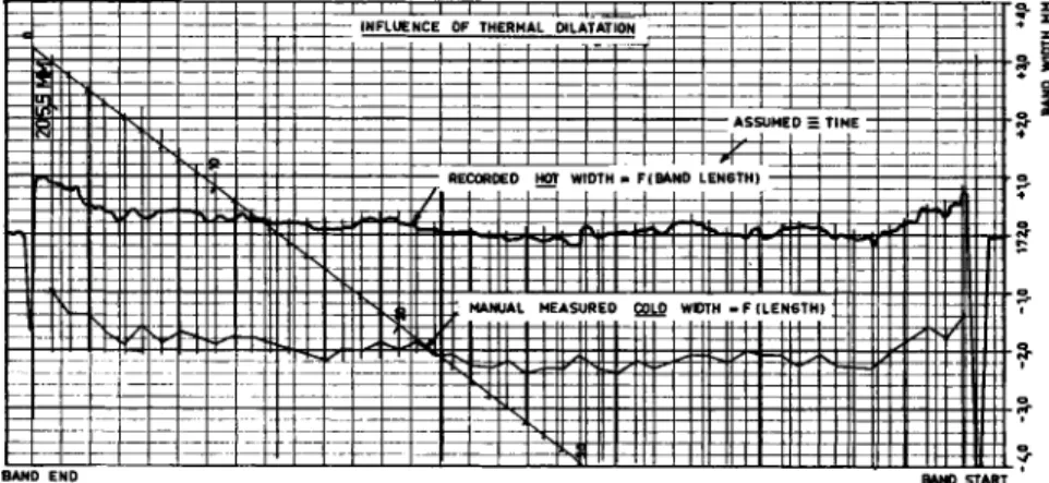
A typical example of a record of the hot width of the strip compared with the manually measured cold width is shown in Fig. 5. The x-axis represents time, which has been taken as being proportional to length in the case of cold measurement. This is true if rolling speed is constant, a point which was not checked in this case. The mean levels, owing to thermal expansion, are displaced by something like 1 per cent of the width. Con- gruence is clear, but the fine structure shown by the recorded hot width is lost in the other measurement owing to the finite number of measuring points. A n interesting feature of the fine structure of the two curves is that the cold peaks are both bigger and more frequent than those of the hot curve.
The explanation of this is either that the high peaks really exist but are of too short a duration for the servo to register them, or, and this is more likely, is largely bound up with the manual measuring accuracy. A n analysis of accuracy will be made later.
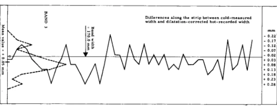
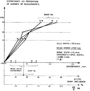
Using a sampling method on the temperature record (20°C intervals) correlated to mean co-efficients of expansion which are already known, a hot-width correction is made. The difference between the corrected hot width and the manually measured cold width is diagrammatically represented in Fig. 6, in which the distribution curve for this difference is also given. Apart from the mean-value discrepancy, which is discussed later, the form of the distribution curve seems to differ slightly from normal
Fig. 5.—Hot and cold width measurement.
of automatic standardization at suitable time intervals for operational checking, could make this instrument a valuable, interference-free tool in the rolling process.
to >
ζ D
Differences along the strip between cold-measured width and dilatation-corrected hot-recorded width
- 0.22 - 0.17 - 0.12 - 0.07 - 0.02 + 0.03 + 0.08 + 0.13 + 0.18 + 0.23 + 0.28
Fig. 6.—Discrepancy between hot and cold width after correction. Mean value = + 0.05 mm.
distribution (this can only be established by comparing a large number of records). The right-hand side is somewhat steeper, indicating better accuracy, either in positive discrepancy measurements for the hot values, or in the negative ones for cold values, or both. Whether one or more systematic errors are involved which could explain this result cannot be resolved without making more elaborate trials. The above-mentioned peaks in the cold width curve may be one explanation, if the positive peaks are higher and/or more frequent than the negative peaks. (Particles in the caliper?) Another explanation is that the mean value of the distribution moves along the length of the strip, having a trend similar to that of the mean value of the total width. This points to a systematic error, influencing the mean-value variation. T o find the origin of this and other sources of error, a trial will be made to distinguish the individual errors.
T w o types of error, the normally distributed errors (denoted by N) and the systematic errors (denoted by S) are included in the overall problem.
A preliminary subdivision gives the following picture:
(a) Apparatus errors, Ν
(b) Deviation from true right angle (2 ways) ± S (c) Temperature-correction errors:
(i) Absolute temperature, S, Ν
(ii) Temp. coefficient//(r, quality)/, N(S) (iii) Light refraction in hot air, 5, Ν (d) Reading-off accuracy, Ν
(c) Standardization errors, 5, Ν
2. Cold reference measuring {sliding caliper) (a) Apparatus error, 5, Ν
(b) Deviation from true right angle (2 ways), ± S 1. Hot measuring
(c) Errors due to surface peaks (irons oxide, etc.), + S (d) Measuring pressure of caliper, Ν
(e) Reading-off accuracy, Ν
3. Evaluation errors
(a) Non-correspondence in location of hot and cold measuring points (time against length scales), S, Ν
(b) Limited number of measurements, sampling, Ν
4. Unknown sources of error
T o evaluate the actual magnitude of all the above errors individually would take quite a lot of time. It is, however, necessary if a given overall level of accuracy must be reached and also if a satisfactory balance between the various sources of error is to be established.
The primary task is to find a figure for the error arising in the hot-meas
uring apparatus (1 a). If all other random disturbing influences are unknown, one statement must be correct: this error must be less than the overall combination of all errors. However, one class of faults can be distinguished, namely those pointing to a systematic displacement of the mean value.
Among these errors (see table) a preliminary appraisal indicates that tem
perature corrections, besides their random errors, also include systematic errors, for example, inaccuracies in temperature readings and adopted coefficients of expansion. This is indicated in Fig. 7, where the mean values and spreads for four strips are marked on the x-axis and j-axis respectively.
DISCREPANCY A S PERCENTAGE OF NUMBER OF M E A S U R M E N T S
Fig. 7.—Fault breakdown with comparisons. Repetition accu
racy. 4 bands at different times;
No. 3, 10, 18, 19. Curves = normally distributed errors: Ο on x-axis = mean value discre
pancy. Cold width = 170.0 mm.
Mean error (for 1 a); Norm, distr. = ±0.1 mm; systematic + spec, distr. = +0.085 ±0.04 (Τ, β).
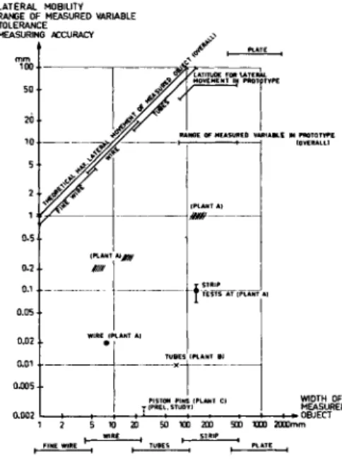
Fig. 8.—Correlation diagram for division into different size ranges, with respective measuring accura
cies, tolerances, ranges of measured variables and lateral mobility of optical width meters.
} χ = measuring accuracy, cold ma
terial; /// = commercial tolerance limits, overall; |β measuring accu
racy, as experimentally determined, hot material. Θ = measuring accu
racy, stipulated hot material. Mea
suring ranges: Meter for plate can for convenience be divided into two instruments with inverted image and integrated double servo units.
The mean of the mean values amounts to about + 0.09 mm with a margin of uncertainty of about ± 0.04 mm, which, if ascribed entirely to tempera
ture error, is equal to 4- 17° ± 8°C. If ascribed entirely to an error in the coefficient of expansion it corresponds to a discrepancy of + 4 ± 2 per cent.
These two examples give a rough idea of how much attention must be given to the different sources of error. The random errors, including practically all "JV" types in the table, can be determined as a half-value figure (inter
section at 50 per cent) or as a one-sigma value (68.3 per cent). The mean value for the four strips is thus less than ± 0.075 mm (50 per cent) or less than ± 0 . 1 mm (1). The qualification "less than", as observed above, is based on the statement that all errors (1-4) are included. Naturally, this maximum figure will never be reached in practical measurement in the mill when only the errors under groups 1 and 4 exert any influence. Even if it is impossible without further analysis to find the absolute values of the faults under groups 2 and 3, a preliminary assumption of equality between the two different main groups, 1 + 4 and 2 + 3 respectively, can be accepted.
This gives a random accuracy (at 1) for the hot-measuring apparatus groups 1 + 4 in the region of + 0.07 mm, which also seems acceptable but which is perhaps a little too good for the reference and evaluating groups 2 + 3 . In conclusion, if the random errors of the apparatus are of the order of the above-mentioned figure ( ± 0 . 0 7 ) , it is clear that the systematic errors not due to the apparatus must be checked and kept within the same order of magnitude before we can reach an ultimate accuracy with satisfactory
balance between the different factors. This balance, however, is also in- fluenced by the costs involved in achieving a given accuracy for the different factors. If as a preliminary attempt, without bringing in the question of cost, the three factors are taken as equal (apparatus error, temperature error and coefficient error) this calls for a temperature accuracy of about ± 14°C and a coefficient accuracy of about ± 3.5 per cent. All these results add up to an overall error of about ± 0 . 1 2 mm, this figure also including the two extraneous systematic errors.
G E N E R A L A S P E C T S
In Fig. 8, an attempt is made to divide the whole width measuring range of interest to steelmakers into practical groups stretching from thin wires up to very wide sheets. The division is primarily based on the following product categories: wires, tubes, strips and sheets. Thus the use of identical loga- rithmic scales on both axes, with the limits of lateral movement, the dynamic measuring range, the commercial tolerances and the experimentally realized tolerances plotted along the j-axis, makes it easy to compare relative figures as between different apparatus ranges. The maximum lateral move- ment in the measuring method discussed above is thus indicated by the 45° line, and the values pertaining to a practical apparatus must lie below this line. The shaded regions, i.e. commercial tolerances, are easily com- pared with the experimentally realised tolerances, and can theoretically be shifted up or down along 45° lines. In practice, however, the trend towards smaller widths is not so steep as 45°. H o w this variation looks for the commercial tolerances can be investigated by collecting figures from a number of plants. For the measuring method dealt with in this article, the trend must also be proved by building small-scale models; in theory the relative accuracy will remain largely constant during the process of scaling down. This means that it is within practical bounds, especially for cold objects, to achieve an accuracy of micron order for measuring widths in the centimetre range. It is scarcely necessary to point out what this would mean for rapid sorting in machine shops, continuous quality control in bar- grinding machines, and numerous other kinds of process measurement and control. The demand for a high-precision non-contact tool for measuring product dimension will inevitably lead to the adoption of solutions based on methods such as that described above.