Electric Vehicles
BMEVIVEM263
Dr.. Gyuláné Vincze
Gergely György Balázs
Electric Vehicles
by Dr.. Gyuláné Vincze and Gergely György Balázs Publication date 2012
Copyright © 2011
Table of Contents
A. List of quantities ... 1
1. Introduction ... 3
2. Traction requirements, selecting vehicle drive ... 5
1. Forces influencing vehicle traction ... 5
2. Designing motive force ... 7
3. Designing brake force in vehicles ... 8
4. Operational modes of vehicle drives ... 9
5. Spinning and blocking of wheels ... 10
3. Types of traction, location and types of traction motors ... 12
1. Electric vehicles with internal and external traction motors and linear motors ... 12
2. Single motor and multimotor drives ... 12
3. Fitting characteristics of rotating motors to traction requirements ... 14
4. Types of electric vehicle drives ... 15
4.1. Using per-unit system for electric machines ... 15
4.2. Park-vector method for invetigating AC machines ... 16
4. Electric vehicles’ energy supply ... 18
1. External and internal energy source ... 18
2. Energy supply of overhead line powered urban electric vehicles ... 18
3. Energy supply of overhead line powered railway vehicles ... 19
3.1. Railway electrification systems ... 20
3.2. Comparing DC and single-phase railway systems ... 21
3.3. Elements of the energy flow at overhead line powered vehicles ... 22
3.4. Multi-voltage locomotives ... 23
3.5. Network-friendly operation for AC voltage powered rail vehicles ... 24
4. Energy supply of levitated vehicles ... 25
5. Energy supply of electric cars and road vehicles ... 26
5. Commutator motor driven conventional electric vehicles ... 27
1. DC commutator motor drives for traction ... 27
1.1. Characteristic curves of the series wound commutator DC motor ... 28
1.2. Control methods of the series wound DC motor in motor mode ... 28
1.3. Electric braking mode of the series wound commutator motor ... 29
1.4. Compound wound commutator DC machines for traction ... 30
1.5. Separately excited commutator DC machine for traction ... 30
2. DC motor driven concrete electric vehicles ... 31
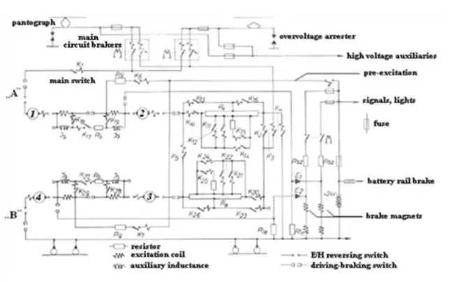
2.1. DC motor driven vehicles operated by series resistance variation ... 31
2.2. Chopper fed DC motor driven vehicles ... 33
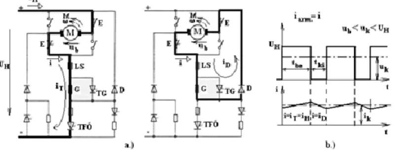
2.2.1. Thyristor chopper controlled DC motor driven vehicle ... 33
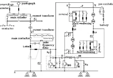
2.2.2. IGBT chopper fed DC motor driven vehicle ... 36
2.3. Diode rectifier fed DC motor driven vehicle ... 37
2.4. Thyristor converter fed DC motor driven vehicle ... 38
2.5. Two quadrant transistor chopper fed DC motor driven electric car ... 38
6. Induction motor driven electric vehicles ... 40
1. The field oriented current vector control theory and practical applications ... 40
1.1. Normal and field-weakening mode ... 42
1.1.1. Maximal utilization of the rotor flux ... 42
1.1.2. Energy-efficient rotor flux control ... 43
2. Voltage source inverter fed induction motor driven vehicles ... 44
2.1. Voltage source inverter fed induction motor trolley-bus drive ... 46
2.2. Induction motor drive system of the Combino tram ... 46
2.3. Voltage source inverter fed network-friendly energy-efficient railway vehicle drives 47 3. Current source inverter fed induction motor driven vehicle ... 49
4. Linear induction motor driven vehicles (LIM) ... 49
7. Synchronous motor driven electric vehicles ... 51
1. Current vector controlled sinusoidal field synchronous motor drive ... 51
1.1. Normal and field weakening mode of the sinusoidal field synchronous drive ... 52
1.2. Voltage source inverter fed sinusoidal field synchronous motor driven vehicles .. 53
1.3. Current source inverter fed sinusoidal field synchronous motor driven vehicles .. 54
2. Rectangular field synchronous motor driven vehicles ... 55
3. Linear synchronous motor (LSM) driven vehicles ... 55
8. Levitated vehicles ... 58
1. Air-cushion levitation ... 58
2. Magnetic levitation ... 58
2.1. Electromagnetic levitation ... 59
2.2. Electrodynamic levitation ... 61
9. Drives of electric and hybrid-electric cars ... 65
1. Electric cars ... 66
1.1. Electric cars with battery ... 71
1.2. Fuel cell electric cars ... 77
1.2.1. Fuel cell energy source for cars ... 77
1.2.2. Application of PEMFC fuel cell in electric vehicles ... 82
1.3. Electric cars with multiple energy storage ... 85
2. Hybrid-electric cars ... 87
2.1. Serial hybrid-electric cars ... 88
2.2. Parallel hybrid-electric cars ... 89
2.2.1. Traditional parallel hybrid vehicles ... 89
2.2.2. Simplified parallel hybrid vehicles ... 90
2.2.3. Two-shaft, parallel hybrid vehicles divided to front and rear axle drives .. 91
2.3. Intelligent hybrid-electric vehicles ... 91
2.3.1. Intelligent hybrid-electric vehicle with planetary gear mechanical drive ... 92
2.3.2. Intelligent hybrid-electric vehicle with Strigear drive ... 95
2.3.3. Intelligent hybrid-electric vehicle realized with double rotor electric machine 96 References ... 99
Appendix A. List of quantities
Name Base unit Used other units or
Comments
t time s h (hour), 1h=3600s
v vehicle speed m/s km/h, 1m/s=3,6km/h
F motive force N kN
Fe running resistance N kN
Fm tractive resistance N running resistance in
horizontal road
Fμ grip limit N maximum motive force
without slipping
m* vehicle mass kg t=1000kg
g gravitational acceleration m/s2 g=9,81m/s2
m*g vehicle weigh N
Θ moment of inertia kgm2 accelerable rotating mass
α gradient angle rad
i* gradient of the road % i*=100tgα[%]
rk wheel radius m
P, p power W kW, LE (Horse power),
1kW=1,36LE
small letter for instantaneous value
η efficiency η ≤ 1
M, m torque Nm small letter for
instantaneous value
ϕ magnetic flux Vs
Ψ flux leakage Vs Ψ=Nϕ, where N is the
number of turns
N coil number of turns
U, u voltage V small letter for
instantaneous value
I, i electric current A small letters for
instantaneous value
R electric resistance Ω
ω angular velocity rad/s n (angular velocity,
1/min), ω=2πn/60≈n/9,55
p* magnetic pole pairs
f frequency Hz
λ wave-length m
s slips
Chapter 1. Introduction
The Electric Vehicles electronic lecture note is made for students of the BME Faculty of Electrical Engineering and Informatics, Electric Machines and Drives MSc branch. The main purpose of this lecture note is to give an overview of the electric vehicles’ drive system solutions, main structural principles, on-board and external joint electric equipments.
Generally the vehicles are the appliances of the public and cargo transportation that possess various size and comfort. The usual categorization with some typical vehicle types is listed as follows:
Vehicle categorization
The drive system solutions of the listed vehicles are disparate therefore these cannot be discussed generally together because these belong to different fields.
This electronic lecture note is only dealing with electric driven land-craft vehicles. Apart from the conventional vehicles it discusses in detail the novel levitated vehicles.
Only those vehicles are called electric vehicles which drive or moving is fully or partly performed by electric motor. Nevertheless all of the modern vehicles contain electric systems with different power level and various electric motor-driven on-board devices; there are numerous vehicles which are not driven by electric motor.
The vehicle design is one of the most complicated engineering creations moreover the vehicles’ electric drive system design is the top of the electrical engineering profession. This lecture note shows the variety, the special features and the specialty of the electric vehicles drive systems and for the easier comprehension it reviews the basic operation of the drive systems. It presents the most typical drive solutions and structures through the examples of concrete electric driven vehicles.
It is assumed that the students possess general electric engineering and basic drive technical knowledge, and they interested in this subject.
The lecture note consists of 8 main chapters.
The 1st chapter is dealing with the tractive requirements of the land-craft vehicles. It shortly summarizes the tractive force, the brake force and the tractive power demands requiring for moving of the vehicles, and other control functions need for safety moving.
The 2nd chapter summarizes the possible tractive methods, the mechanical drive system solutions and the electric motor implementation of the land-craft vehicles. The chapter gives an overview of the electric drive system sizing for given tractive demand.
The 3rd chapter presents the electric vehicles’ power supply methods. Larger part of this chapter is dealing with the overhead line power supply systems and the requirements of the network friendliness but other power supply methods are reviewed also, including the power supply of the levitated vehicles.
The 4th chapter presents the conventional brush-commutated DC motor driven public transport and rail vehicles through some vehicle examples.
The 5th chapter is dealing with the field orientated, inverter-fed induction motor drive systems, used for traction and presents some concrete vehicles equipped with modern drive system.
The 6th chapter presents the field orientated, inverter-fed synchronous motor drive systems, used for traction.
The most interesting application, the linear synchronous motor traction is detailed.
The 7th chapter is dealing with the levitation methods and special problems of the levitated vehicles.
The 8th chapter is focusing on the drive system technics of the electric and hybrid-electric cars.
The following key words are used in this lecture note:
1. The vehicle electric drive performs the moving of the vehicle. The electric drive contains the electric motor, the power electronic circuit and the control and protective devices.
2. The main electric circuit consists of the electric circuits of each element required for the vehicle traction and operation.
3. The auxiliary devices are not involved in the vehicle traction. These devices are for signaling, controlling, protecting, information transferring and comfort, heating and cooling.
4. The auxiliary circuit consists of the electric circuits of each element performing operation of the auxiliary devices.
Chapter 2. Traction requirements, selecting vehicle drive
1. Forces influencing vehicle traction
Forces acting in vehicle movement can be divided into four groups:
1. forces pointing parallel to vehicle movement, 2. forces perpendicular to path of motion, 3. lateral forces acting on the vehicle, 4. inertial forces influencing the movement.
Forces a), b) and c) arise between the path (or medium of movement) and the vehicle.
Secure movement can be realized with strict monitoring and controlling the above forces. Main requirements of secure movement are:
1. vehicle moves with the expected constant speed and direction on straight-line path, it does not slip during acceleration or deceleration.
2. It does not (or with allowable degree) leave the planned path during change of direction.
3. canting, pitching and oscillation of vehicle body is damped properly and kept to acceptable level under operational circumstances.
Vector sum of active and passive forces pointing to movement direction determines whether vehicle accelerates, decelerates or moves with constant speed.
Active force in the movement direction can be:
1. motive force (pushing or pulling) F acting in the movement direction controlled by the vehicle driving engine and
2. brake force F brake acting on opposite direction, controlled by several braking actions.
In vehicles rolling on wheels, motive and brake force acts between the path and the surface of the wheels and depends on the adhesive conditions. Such a limit does not appear with levitated, linear motor-driven vehicles.
Passive force in mov ement direction is the vector sum of forces acting against the movement. Force opposite to movement is so-called tractive resistance F m. Most part of tractive force is air resistance (windage), which depends quadratically on vehicle speed, usually. Also, part of the tractive resistance is the rolling resistance and, in case of levitation, the so-called magnetic resistance depending on levitation mode. If the gradient angle of the path is α then gravitational force m * g calculated from the vehicle mass m * has passive component m * gsinα parallel to the movement, which is opposite to movement when climbing up and in the same direction (additional) when going down the slope. Gradient of the road is given by tgα: i * =100tgα[%].
Figure 1-1. Forces acting parallel and perpendicular to movement path
Vector sum of active and passive forces in the movement direction determines acceleration of the vehicle dv/dt:
1-1
m* red is resultant accelerated mass of the vehicle. If we have to accelerate a rotating mass inside the vehicle, for example the motor with inertia Θ m, resultant mass is m* red≥m*, where m* red=m * +(ω m 2 /v 2 )Θ m. (ω m: rotational speed of motor).
1. If F=F m +m*gsinα, which means that motive force equals to passive forces, then vehicle moves with constant speed, its acceleration is zero.
2. If F>F m +m*gsinα, then vehicle accelerates, if F<F m +m*gsinα, it decelerates.
3. If F goes to negative, then vehicle is in brake mode.
Forces acting perpendicular to movement path cannot be controlled in most of the land crafts, which transfer to road or rail. Exceptions are levitated vehicles.
Passive forces perpendicular to movement has two components, gravitational force pointing down, and lifting force pointing up. Gravitational force is usually much bigger. On horizontal surface, the whole weight of vehicle m * g acts perpendicularly to path, on non-horizontal surface only its perpendicular projection m * gcosα, as can be seen in Figure 1.1.b. Lifting F lf force is a component of air resistance and depends on the shape and speed of vehicle.
Controllable perpendicular active forces arise only in levitated vehicles. If active levitation forces equal to passive forces, then levitation distance is constant, otherwise the distance changes.
At traditional vehicles moving on wheels, sum of forces perpendicular to path (m * gcosα-F lf) play an important role. Part of this force G w appearing on one wheel presses the wheel to the road, and this force determines the possible tractive and brake forces. Circumferential force F tk that can be transferred on one wheel depends on pressing force and grip coefficient μ w of the wheel (k is number of wheels):
1-2
μ w grip coefficient depends on the conditions of the road and wheel, weather, velocity of the vehicle and is different for each wheel, usually. Sum of the transferable forces F t is limited because of the limited gripping coefficient, F t ≤F tmax. An ideal tractive (or brake) force can be calculated for vehicles with wheels, which can be transferred to horizontal road (α=0) with low speed (F lf ≈0), in good road conditions and dry weather. This ideal force is called gripping limit, F μ:
1-3
If tractive force of the motor or brake force of the brake system is lower than the limit, then traction is realized with normal rolling. If tractive force is higher than momentary transferable force F t, then wheel spins, if brake force if higher, then wheel blocks (see more details in Section 1.5). Such spinning or block effect does not appear in levitated vehicles.
Lateral forces cannot be controlled in most of land crafts, they are passive forces and are transferred to the road or rail. Rail or wheel counteracts these forces coming from turning or side-wind.
However active controlled lateral forces are needed to counteract lateral passive forces in levitated vehicles or to control lateral movement.
Inertial forces influencing movement of the vehicle body generate canting, pitching and oscillation of the body.
Dumping of these forces is required for stabilization of the vehicle. There are special solutions for damping and stabilization.
Traction requirements, selecting vehicle drive
2. Designing motive force
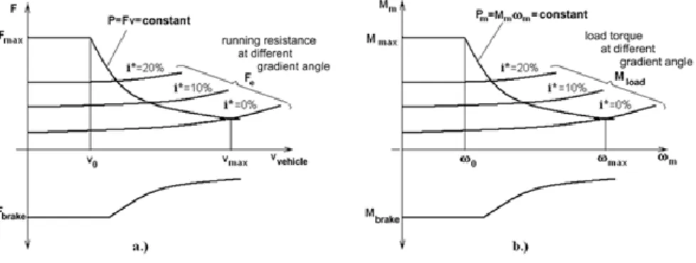
Acceleration of a vehicle dv/dt with mass m * is determined by the vector sum of active and passive forces in the movement direction, as can be seen on equation (1.1). Force m * gsinα resulting from the gradient of the road depends on what terrain the vehicle is designed for. Tractive resistance F m is determined by the type and shape of the vehicle and increases non-linearly with velocity. Sum of the passive forces is called running resistance F
e, where F e =F m +m * gsinα. Running resistance vs. velocity for different road gradients are shown in Figure 1.2.a. Tractive resistance F m can be got from running resistance F e where gradient i * =0%.
Figure 1-2. a./ Parallel forces b./ Tractive power needed
Figure 1-3. Acceleration of vehicle vs. time, with maximal tractive force and i*=0%.
From the viewpoint of motive force, vehicle drive has to be designed so that motive force available is greater than running resistance characteristic used for design in the whole velocity range. Based on equation (1.1), acceleration reserve is the difference of momentary motive force and running resistance F-F e. If the available motive force of the vehicle drive is that shown in Figure 1.2.a. then acceleration reserve is the greatest at starting and reduces to zero when v=v max, on a horizontal i * =0% road. Final speed on a horizontal road is limited by this, as motive force F is not greater than momentary running resistance F e,vmax, i.e. the vechicle cannot accelerate. In this operating point, motive power required to keep velocity v max is:
Drives are designed for this final P=P motive,max power, and this designed power is usually available in a wide range of velocity, as can be seen in Figure 1.2.b. Motive power is constant in a wide velocity range if P=Fv is constant, which means that motive force decreases hyperbolically when increasing velocity. Constant power range can be used until maximal motive force F start, i.e. between v 0 and v max. F start is calculated from the required starting acceleration (according to equation 1.1). Gripping limit calculated in equitation 1.3 shouls also be taken into account when designing vehicles running on wheels, as motive force greater than grip limit cannot be transferred via wheels.
Such an ideal motive force characteristic can be seen in Figure 1.2.a. This characteristic, of course, is a limit characteristic. Under this curve, motive force has to be controllable freely, according to the demanded
momentary acceleration. A starting and acceleration process, which takes full advantage of the ideal motive force curve, can be seen in Figure 1.3. Motive force F is set to value F e,vmax when final velocity is reached, and acceleration reserve decreases to zero. Dynamic behavior is usually described by starting acceleration value v 0 /t
0. Acceleration that can be seen in the figure is used rarely; instead, softer acceleration is used that is more convenient to passengers.
Motive force and running resistance of different vehicle types are shown in Figure 1.4. and 1.5.
Figure 1-4. Specific tractive characteristics of urban vehicles
In the figure, specific motive force and power characteristics are shown, relative to vehicle mass m *.
Urban vehicles are designed for relatively low speed and high gradient angle. For example, angle i *=20-25% is used for garage ramp, and this slope must be performed.
Figure 1.4 is prepared for urban vehicles and gives minimal motive force and power that have to be taken into account during design.
Figure 1.5 shows motive force characteristics of locomotive series V43, popular in Hungary, for two different gradient angles and pulled masses.
Figure 1-5. motive force characteristics of locomotive series V43.
Locomotive was designed for various applications (goods, slow and express trains). Allowable starting force F
start is limited by grip limit F μ in equation (1.3).
Characteristics of motive force of engines with maximal voltage and current are indicated by lines 1 and 2. Line 1 is for maximal excited motor, and line 2 is for maximal allowable field weakening (42%).
Motive force range under line 3 can only be used for continuous and long time mode, under motive force F hour. Constant motive power is used between points A and B. Motive force for momentary acceleration demand can be set with voltage regulation and field weakening under limit characteristics. Voltage of the motor and field weakening can be changed with steps for locomotives V43.
3. Designing brake force in vehicles
In every vehicle, at least three independent brake systems must be used for security reasons:
1. normal operation brake system,
Traction requirements, selecting vehicle drive
2. security brake system, 3. arrester brake.
Arrester brake secures the vehicle in standing position without additional energy supply.
Normal operation brake in an electric vehicle is realized with controlling brake mode of the driving electric motor, almost without exception, despite of the fact that brake effect can only arise on driven wheels in case of vehicles running on wheels. (In case of levitated vehicles, brake mode of driving linear motor can affect along the whole length of the vehicle.) Brake mode of an electric drive can be lossy, or lossless, with regenerated energy. In modern vehicles, regeneration of braking energy plays an important role during design. Brake with loss (realized with resistance) is only used if regeneration cannot be used because of some reason. In regeneration brake mode, brake force is limited by maximal regeneration brake power and maximal brake force, just like during traction mode (Figure 1.6).
Figure 1-6. Tractive characteristic extended to brake mode
Novel electric vehicles are designed so that the whole energy can be regenerated, i.e. regenerated power equals to the used power during traction.
Energy saving that can be realized with regeneration is 5…35% of the input energy, depending on the road conditions and number of stops.
Security brake system is always mechanical and not electric. Hydraulic or pneumatic frictional brakes are used in vehicles with wheels and they are mounted on all wheels. In levitated vehicles, air resistance is increased to provide mechanical brake, this solution is called aerodynamic brake.
Normal mode and security brake systems are separated in most vehicles, and can be operated jointly or separately. Brake control is designed so that joint total brake force by normal mode and security brake should be controllable, too, and brake force should be developed continuously, without steps.
Control of brake has several aims:
1. to stop the vehicle securely,
2. to set a comfort deceleration in time for the passengers, 3. anti-blocking of the wheels, in case of vehicles with wheels.
4. Operational modes of vehicle drives
Motive and brake force are opposite, as can be seen in Figure 1.6. In the figure it is not indicated, but most vehicles has to be able to move forward and backward. Operational modes needed for traction can be seen in Figure 1.7.
Figure 1-7. Operation modes, 4/4 quadrant operation
In I and III quadrant of a general 4/4 quadrant mode, the motive power is P=Fv>0, in this case drive operates as a motor. In II and IV quadrants P=Fv<0, in this case drive operates in brake mode. Modern vehicle drives can change between quadrants without mechanical or electric switches, i.e. drive is also 4/4 quadrant. There are drives suitable only for less quadrants. For example, internal combustion engines can operate only in one quadrant, forward and backward reversal has to be done mechanically and brake is realized only mechanically, except power brake.
5. Spinning and blocking of wheels
Force that can be transferred on the surface of the wheels depends on force pressing the wheel to the road and the gripping coefficient, according to equation (1.2). There is a nonlinear relation between the motive force required for traction and force transferable with wheels, as can be seen in Figure 1.8.a.
Figure 1-8. Grip characteristics, a.) transferable motive force on wheels, b.) grip limit vs velocity
As the figure shows, transferable force follows the required value, indicated with dashed line, but curves separate sooner or later, depending on weather conditions. Until transferred force can follow the required force, the vehicle is in normal rolling mode (with small slip). In this case the difference of the two forces is the rolling resistance, which depends on wheel deformation, wheel and road conditions and speed of the vehicle. Increasing the required force (engine torque, brake force), rolling friction becomes slipping friction, and transferable force becomes smaller than required, and it has limit value. Momentary limit Ftmax, indicated in Figure 1.8.a, highly depends on weather and other conditions. The biggest from these limits is the gripping limit F μ indicated in equation (1.3).
Gripping limit depends on vehicle speed, decreases when velocity increases, as can be seen in Figure 1.8.b. It has two reasons. One is that lifting force, ignored in equation (1.3), increases with higher speed, so force pressing the wheels on the road decreases. Another is that the effect of road rugosity becomes more and more higher when speed increases, wheels often move off the road. As gripping ability decrease with speed, and rolling resistance increases, a speed limit (300-350 km/h) has to be used for traditional trains.
In traction mode, force higher than transferable (shaft torque/radius) spins the wheels, and blocks the wheel in brake mode. Both effects are harmful, so control of traction and brake force has to be used. To characterize spinning and blocking, relative slip of a wheel is defined as follows:
1-4
Traction requirements, selecting vehicle drive
where v circ is circumferential speed of the wheel (Figure 1.9.b). To calculate slip precisely, we should know the speed of the vehicle even if spinning has already started. In practice, angular velocity ω w is measured and circumferential speed can be calculated as v circ =r w ω w. Speed of the vehicle can be calculated with average angular speed (ω av ):
1-5
where r w is radius of wheel, k m is number of measured wheels. Calculation is less accurate if more than one wheel slides and another uncertainty is the radiussince wheel can deform during wear and load. v circ >v road (see Figure 1.9.b) and s>0 during sliding, and v circ <v road and s<0 during blocking, where v road =-v vehicle. Figure 1.9.a shows the relation between the absolute value of relative slip and gripping coefficient. This relation is similar to all vehicles running on wheels, but μ and s values can change significantly, for example for vehicles running on rail or road. A short slip range can be determined for a vehicle type where there is a linear relation between gripping coefficient and slip. This range is the range of normal rolling. If gripping worsens, relative slip goes outside of this range (as an indicator) in case of spinning or blocking.
Figure 1-9. a) Grip coefficient vs relative slip, b.) spinning, c.) blocking
Anti-spin of wheels operate in tractive mode and the torque of traction motor(s) is controlled (limited). Anti-spin system limits the torque so that relative slip is inside the narrow range shown in Figure 1.9.a, i.e. wheels can roll and transfer force to the road. The role of anti-spin is to prevent spin of wheels and, in case of rails, to protect rails and wheels. Wear of rails in case of spinning or blocking is a problem in high-speed trains at stations and places where stop and start happen often. To increase grip, sand technique is often used for vehicles running on rail.
Anti-blockin g of vehicles running on wheels operates in brake mode and (total) brake force is limited in case of using several brake systems. There are two goals of anti-blocking. In case of rails anti-blocking is designed to prevent slipping to protect rail and wheels and to ensure rolling of wheels. In case of tyres, anti-blocking system limits brake force so that transferrable brake force on wheels should be maximal. This goal can be reached with about 5% relative slip where gripping is maximal. Such a brake force control is called ABS.
(References used in this section are: [1]…[5])
Chapter 3. Types of traction,
location and types of traction motors
1. Electric vehicles with internal and external traction motors and linear motors
In a vehicle with internal traction motor one or more electric traction motors are placed “on-board” with all auxiliary mechanical elements (mechanical drive, gear, shock-absorber). Motor increases the mass of the vehicle. Most of the vehicles are equipped with internal and rotating motors.
In a vehicle with external traction motor the traction motor is placed into an engine room outside the vehicle body, its mass does not loads the vehicle body. Instead, engine room, traction mechanics, tow rope and suitable track is needed for the traction of the vehicle.
Traction motor of l ine ar motor vehicles is placed partly on the vehicle and partly on the track. In this construction, mass of motor inside the vehicle can be much lower than in vehicles with internal motor. Contrary, trail needed for linear motor drive is more complicated and expensive than trail of traditional vehicles. Linear motor drive is usually used in levitated vehicles. Motive force arises between the two parts of the linear motor without mechanical connection.
2. Single motor and multimotor drives
Most of the land crafts roll on wheels and are driven by internal rotating motor. The number of wheels and mechanical solutions for traction are very different in vehicle constructions. Regarding the number of motors the vehicle can be driven by a single motor or multimotor.
Single motor vehicle can be designed if requirements for motion force and traction power can be fulfilled with one motor.
Single motor vehicles can be divided into three groups:
1. electric cars, hybrid buses, trolleys,
2. electric bicycles and other low power electric vehicles, 3. linear motor vehicles, as a special case.
The construction of the vehicles in the first group is usually similar to vehicles with internal combustion engine, and electric motor is connected to front or back wheel axles with cardan shaft and differential gear (Figure 2.1.a). Gearbox with variable transmission and clutch is not needed in electric vehicles.
If there is a fix transmission between the angular speed of motor and wheels then this transmission is required to fit the angular speeds. In low power vehicles even simpler, v-belt or chain-drive is used, or a wheel hub motor placed on the wheel with flat, disc-type shape.
Figure 2-1. Drive of electric cars, a.) single motor drive, b.) wheel hub motor drive
Vehicles with linear motor drive can be considered as special single motor vehicles where motor is along the whole body.
Types of traction, location and types of traction motors
Multimotor drive can be used in low or high power vehicles, too.
An example for multimotor low power vehicle is an electric car with separately controllable wheel hub motors in every wheel (Figure 2.1.b). Usually, rpm of the motor and the wheel are the same. Motors drive the wheels directly and not the axle. Such a drive has mechanical problems as mass of wheels increase, and there is a flexible connection between rotor and stator of the motor.
There are several reasons to design high power multimotor vehicles:
1. One reason is electrical and is based on conventions. Voltage on one motor can be changed with serial or parallel connection of the motors. Changing serial and parallel connections of two motors is used in two- motor trams and underground trains, for example.
2. The other reason is mechanical. When using more motors construction can vary. Motive force can be divided to several wheels, power required for traction can be divided between motors, and more, smaller motors are easier to place inside the body.
Typical multimotor vehicles are electric locomotives where motors are placed on bogies, in several variations. A common sign system is used to indicate the mechanical solution. For example, B’B’ sign means vehicle with two bogies with two-two pair wheels and one motor per bogie, BoCo sign means two bogies with two wheel pairs on one bogie (sign B) and three on the other (sign C), and every wheel pairs driven by separate motors (index o), which means 5 motor drives altogether.
Figure 2.2 shows driving motor placed on wheel axle. There is a connection with rubber core and cardan shaft between the motor and axle which enables flexible displacement.
Figure 2-2. Unique axle drive of BoBo axle arrenged locomotive series 1047
Point of interest of this solution is that there is a separate brake axle to place the brake discs which connects to the axle of the motor through the “big gear”. In this way, motor is not influenced by the heat of brake discs.
Novel multimotor drive solutions can be found in low floor urban/suburban vehicles. Because of low floor (350 mm or below step-in height), wheels on the left and right cannot be connected with axle, contrary to locomotives. Novel types axles are required.
A low floor vehicle with two-two wheels behind each other with common drive can be seen in Figure 2.3.
Examples for this solution are Swiss made COBRA and Combino trams running in Budapest. There are electric motors on left and right sides which drive two wheels on the same side (indicated with yellow in the figure) with two-side cardan axles. There are seats above the wheels. A specialty of vehicle COBRA shown in figure 2.3 is that its axles are steered mechanically (automatically from the side of the vehicle), and this solution provides exceptional advantages in curves, regarding to wear and noise.
Figure 2-3. a. Low floor vehicle with common side wheel drive, schematic
Figure 2-3. b. Low floor vehicle with common side wheel drive, látványkép.
Low floor vehicle with wheel hub motor is shown in Figure 2.4. An example for this solution is Variobahn vehicle developed by ABB(Adtrans). Wheel hub motor has outer rotor, its stator is inside (Figure 2.4.b).
A special type of multimotor vehicles is a hybrid-electric vehicle, where internal combustion engine can also participate in driving besides the electric motor, at the same time.
Figure 2-4. Low floor vehicle with wheel hub motor, a.) schematic, b.) realization
3. Fitting characteristics of rotating motors to traction requirements
Traditional cylindrical rotating machines are designed for high rotational speed so that their diameter would be the smallest possible. This rotational speed is 6-7000/min for vehicle motors, or 6-700 rad/s as angular speed.
The fixed ratio r=ω m /ω w between angular speeds of motor ω m and wheel ω w must be set so that maximal motor rotational speed corresponds to final speed of the vehicle.
Calculating speed of vehicle v from angular speed of motor is shown in (2.1.a), where r w is radius of the wheel.
This calculation is for ideal conditions, assuming that there is no slip, spin, so circumferential speedof wheel r w
ω w equals to vehicle speed.
2-1 a.
2-2 b.
Types of traction, location and types of traction motors
The expression between the torque of motor M m and its motive force is shown in equation (2.1.b). Losses of the drive can be taken into account with efficiency η<1. One motor can drive several wheels, in this case motive force (2.1.b) is distributed among the wheels, for example among the two driven wheels in Figure 2.1.
If several motors drive the vehicle then motive forces of the motors are summarized in a way that angular speed ω w of the wheels are constrained through the road. A problem can be to distribute the load among the motors equally, there are different solutions for this in different vehicles.
Variable transmission gearbox used for internal combustion engine drives can be eliminated if the mechanical characteristic M m -ω m of the electric drive fits to traction need F-v of the vehicle without modification. Fitted characteristic M m -ω m of the electric motor means that all of its points, calculated as above, suits to ideal traction characteristic, as shown in Figure 2.5. Load torque characteristics calculated from running resistance to motor axle is also indicated in Figure 2.5.b.
Figure 2-5. Fitting the drive a.) motive demand, b.) mechanical characteristic of traction motor
Electric power P m =M m ω m required for traction can be calculated from tractive power P=Fv, taking into account drive losses:
2-2
Power P m is the sum of the powers of the motors in case of a multimotor solution. In this case, we have to take into account that the distribution of loads among the motors are not even, for example load can be higher than average because of the wear of the wheel. Differences must be taken into account when designing the motors.
4. Types of electric vehicle drives
As can be seen above, drives with mechanical characteristic fulfilling the requirements indicated in Figure 2.5.
can be used for traction without mechanical gear.
The following drives can be used:
1. serias excited DC motor drive with commutator, extended with field-weakening range;
2. inverter-fed field-oriented controlled induction motor drive, extended with field-weakening range;
3. inverter-fed current vector controlled, permanent magnet, sinus-field synchronous motor drive, extended with field-weakening range (PMSM drive);
4. multi-phase, permanent magnet, rectangle field synchronous motor drive (so-called ECDC or BLDC drive);
5. switched reluctance motor (SRM) drive (rarely).
Earlier, one-phase commutator motor drives were also used, but not nowadays.
4.1. Using per-unit system for electric machines
To simulate the behaviour of electric machines, per-unit system is often used. With per-unit system, several behaviours and control modes can be compared easier, and it is also easier to evaluate the simulation results.
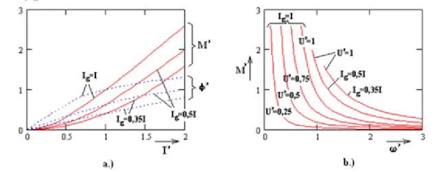
The quantities in per-unit indicated with superscript comma express relative values related to nominal values indicted with index n. Important per-unit quantities for DC machines are: I’=I/I n, U ’ =U/U n, ϕ ’= ϕ / ϕ n, M ’
=M/M n, where M n is nominal torque determined by ϕ n and I n.
4.2. Park-vector method for invetigating AC machines
This section summarizes the basics of Park-vector method used for three-phase AC electric machines, as it is required for the further parts of this book.
Three-phase electric machines are usually described by voltage, flux and torque equations. Original equations for phases a, b, c form an equation system where interactions between phases are also described. This equation system is hardly usable because of inductive couplings. As interactions are cyclic and symmetric in three-phase machines, a transforming method is available where vector based descriptions are available instead of phase quantities. The advantage of this transformation method is that three phase equations are simplified to two equations (without coupling between them): equations for Park-vectors and zero -sequence components.
Equation for zero -sequence components can be eliminated if (i a +i b +i c )=0 is fulfilled with construction, for example in machines with star connected winding and not-connected star point.
Vector description is made with Park-vectors calculated with operators (1, ā, ā2), where
and .
Vector description of three-phase electric machines uses the vectors constructed in the way etc., where u a , u b , u c , i a , i b , i c etc. are instantaneous values of phase quantities. Using these vectors a Park-vector based equation system can be created.
Park-vector equations describe the system unambiguously if inner or outer zero-sequence component voltage u
0=(1/3)(u a +u b +u c)≠0 cannot create zero -sequence current i 0=(1/3)(i a +i b +i c), as (i a +i b +i c )=0 requirement is fulfilled with construction.
Figure 2-6. Current Park-vector
Park-vectors calculated as above are complex quantities resulting from the transformation, and their real and imaginary components, magnitude and angle can be calculated in every moment. Advantages of vector description are that vectors can be drawn in plane field, and momentary quantities are easy to calculate. For example, knowing current vector ī phase currents i a , i b , i c can be calculated, as shown in Figure 2.6.
Instantaneous three-phase quantities can be calculated from a vector in every moment with a simple projection rule; they can be calculated from the projections to the a, b, c axes (1, ā, ā2 directions). In the example, i a is positive, while i b and i c are negative and have almost half values, comparing to i a.
Transient processes of three-phase electric machines can be represented easily with Park-vectors, and vector description provides possibility to coordinate transformation, for example to rotating coordinate system.
Calculating electric power with Park-vectors
Instantaneous power described with phase voltages and currents is:
Types of traction, location and types of traction motors
2-3
Park-vector description of the same power, together with zero -sequent components u 0=(1/3)(u a +u b +u c) and i
0=(1/3)(i a +i b +i c), is:
2-4
In this equation dot means scalar product, i.e. ū·ī=│ū│·│ī│cosφ, where φ is the angle between voltage and current vectors. As i 0=0, usually, zero -sequent power component, the second part of equation (2.4) is often not indicated.
(References used in this section are: [6]…[9])
Chapter 4. Electric vehicles’ energy supply
1. External and internal energy source
The electric energy supply of the electric vehicles is performed by the following three methods:
The external energy supply is generally the national electric energy network directly or converted by intermediate devices. The vehicle is operable if the energy transmittance is fulfilled. The energy transmission can be fulfilled by a trolley contact at vehicles powered by overhead-line. At inductive energy supply the transmission is fulfilled by induction without connections. Basically there are three types of vehicles powered by overhead-line: electric vehicles of the urban public transport (tram, trolley), urban rail vehicles (metro, suburban railways) and railway vehicles. Inductive energy transmission can be found at high-speed linear motor driven vehicles. The solar cell is a special solution for the external power supply.
Most commonly the battery is t he elec t r ic energy storage device that is delivered by the vehicle. The stored electric energy is applicable for the traction of the vehicle (electric car, forklift truck) or in most of the cases it powers just the auxiliaries. Apart from the batteries, ultracapacitors or fly-wheels can be applied independently, or as a secondary energy storage device. The conditions of the energy storage devices shall be continuously checked, the recharging should be provided periodically.
The diesel-electric locomotive is operated by chemical energy delivered o n the vehicle. A diesel aggregator is the electric energy source of a diesel-electric locomotive. The hybrid-electric vehicle is similar. Its design is based on different combinations of internal combustion engine (diesel or Otto-engine) and electric generator.
The fuel-cell can be the power source of a vehicle that is operating with hydrogen (sometimes with methanol).
Gas turbine powered electric vehicles also exist. At the former mentioned vehicles the stored chemical energy is transformed to electric energy on-board. The refueling of these vehicles should be provided periodically.
The range of the vehicle is the maximum route that can be achieved by a “non-external energy powered” vehicle with one energy charge.
2. Energy supply of overhead line powered urban electric vehicles
The urban electric vehicles are operating with DC voltage network. The nominal voltage of the overhead line is different. For example in Budapest: 600V (tram), 825V (metro), 1100V (suburban train), 1500V (cog wheel train), the permissible voltage range from the nominal value is +20%...-30%. In urban traffic conditions it is characteristic when the stops and the reasons that stop the vehicle are frequent therefore the load of the overhead line is dynamically varying. Between two stops launching, accelerating, coasting, braking, stopping, waiting phases are repeating. For energy saving purposes the power-off coasting - that has no energy demand - and at modern vehicles the regenerative braking is the often used. With regenerative braking the 20-30% of the energy consumption of the urban electric vehicles can be saved.
Electric vehicles’ energy supply
Figure 3-1.: Energy supply of urban electric vehicles a.) substation, b.) tram, c.) trolley.
The DC voltage of the overhead line is produced by a diode rectifier circuit connected to the three-phase public supply network through a transformer (Fig.3.1.a). Therefore the vehicles cannot recuperate the braking energy into the public supply network. Considering the fact that in urban traffic a few vehicles powered from the same contact line, the energy transmission can be achieved between the vehicles. Therefore the recuperated energy (current) of a braking vehicle can be consumed by other vehicles. In the aspect of the vehicles the regenerative braking mode can be achieved, if provided that the contact line voltage not exceeds the permissible value. If the maximum voltage level is reached, other braking mode should be selected e.g.: resistive braking.
The contact line is generally overhead line (Fig.3.1.b.), at trolleys two overhead lines (Fig.3.1.c.). The energy is supplied by a third rail at the metro and the millennium underground train. The contact line is distributed to segments that can be separately released, the energy supply of the segments can be unidirectional or bidirectional. The energy supply of the busy, radial-connected junctions causes problems for the urban vehicles.
3. Energy supply of overhead line powered railway vehicles
Public network connected high power substations are established along the railway track in defined distances for supplying the overhead line powered railway vehicles. All the switching, converter and protecting devices are in the substations that are required for the overhead line supply.
The following table summarizes the railway overhead line systems, the vehicle drive system solutions and the required energy converters. According to the table there are several solutions, each electric traction mode need several energy conversion processes, therefore for the traffic designers it is difficult to find the optimal solution.
Table 3-1.: Contact line voltages and electric energy conversion solutions.
Main converters of the substations Overhead line voltage Internal energy consumption:
electric drive and the required internal energy conversion
transformer +
phase change among segments
single-phase, standard frequency voltage
(each of the listed vehicle drives is equipped with built-in transformer, that has suited-voltage and galvanically isolated)
1. DC motor with rectifier and split transformer
2. DC motor with controlled rectifier
3. AC drive with DC-link frequency converter The DC-link can be:
transformer single-phase, low-frequency
voltage
The application is similar to the former
+
frequency converter
(nowadays the single phase brushed DC motor without rectifier is not used)
transformer +
rectifier
DC voltage (the vehicle drive is not galvanically
isolated from the contact line) 1. DC motor with switchgears,
resistor gears
2. DC motor drive with DC chopper 3. AC drive with DC-link frequency
converter
transformer three-phase voltage induction motor drive with gear-
switches (Italian Kandó-system, it is not used nowadays)
3.1. Railway electrification systems
Features of the overhead line powered systems: supply voltage amplitude, number of the phases and the frequency; at railway applications these three together is called “current type”. Several railway electrification systems exist all over the world. If a vehicle can operate in two different systems it is called dual-voltage vehicle. In Europe six different railway electrification systems have been evolved because in different countries the railway electrification had begun separately under various conditions:
1. DC, 850 V: England
2. DC, 1500 V: France, Netherlands
3. DC 3000 V: Spain, Belgium, Italy, Poland, Slovenia, Czech Republic, Slovakia
4. three-phase, AC: Italy (nowadays it is not used because of the problems of the current collection) 5. single-phase, AC, 15 kV, 16 2/3 Hz: Austria, Switzerland, Germany, Sweden, Norway
6. single-phase, AC, 25 kV, 50Hz: Hungary, France, Denmark, Great-Britain, Czech Republic, Slovakia, Croatia, Yugoslavia, Romania, Bulgaria
The content of the former list continuously changes because of the reconstructions and the installation of new systems. According to the list, in practice the voltage of the overhead line system is DC voltage or single-phase AC voltage (three-phase overhead line is already not used). Two different types of the single-phase system exist:
the standard frequency and the low-frequency. It is possible when two different electrification systems can be found in one country. In each European country at the installation of the modern high-speed railways the 25kV, 50Hz supply system is used.
The following diagram presents the distribution of the European railway electrification systems. According to this diagram the ratio of the different systems is approximately the same, except the 850V DC system. This causes a significant problem at the transcontinental traffic because locomotive must be changed at the border of different electrification system that can take quarter an hour which increases the travel time.
Electric vehicles’ energy supply
Distribution of the European railway electrification systems
Installing a unified European railway electrification system is not feasible because of several reasons. If either system is selected at least 67% of the European electrified lines should be adopted. It requires significant cost;
moreover numerous devices (converters, supplying systems, substations, etc.) would become unnecessary.
Perhaps these devices operate at the beginning of their life cycle or could be expensive. More than 50% of the electric locomotives would become inappropriate to operate causing lack of locomotives; moreover it would result in disturbances of the railway traffic. Adopting needs extremely great cost; moreover it should be performed in a short time, just in a few days.
The cheaper solution is to buy tractive vehicles that can operate under different electrification systems. These are called dual-, triple- or quad-voltage locomotives. These shall stop for a short period at the border of the different electrification systems and switch to the proper system by keeping appropriate rules. This can be executed in one minute; therefore it does not cause significant loss of time.
3.2. Comparing DC and single-phase railway systems
The DC railway electrification system has been evolved for DC traction motors. The 1500V voltage value was defined by the maximum permissible nominal voltage of the DC motor commutator bar voltage. The 3000V DC overhead line voltage is applicable if at least two motors are always connected in series. The low voltage level is a great disadvantage of the DC system, therefore a few thousand ampere current supply shall be provided for the high power traction. While at direct current the voltage drop of the current conductors is resistive, such a large current causes large voltage drop even in increased diameter contact line (500-600 mm2). Therefore the energy supplying substations shall be installed relatively densely, at 1500V systems the distance between two substations is 10-15km.
In the past, at the substations the DC voltage was generated by synchronous motor driven DC generators.
Nowadays it is generated by a diode rectifier connected to the public supply network through a matching transformer. Generally the contact line is at positive polarity, the rail is at negative polarity. If DC voltage supplying substation is installed by a rectifier, the braking energy cannot recuperated into the public supply network. The energy transfer is limited but it can be achieved by two vehicles connected to the same contact line. Therefore the recuperated energy (current) of a braking vehicle can be consumed by other vehicles connected to the same line and operating in motor mode.
The contact line is distributed to segments that can be separately released, the energy supply of the segments can be unidirectional or bidirectional.
Sing le-p hase AC supply system can be operated with standard frequency or low-frequency. The nominal value of the overhead line voltage can be high (in Hungary: 25kV) and it is a great advantage of the AC systems. The built-in main transformer of a vehicle produces the most adequate voltage level for the electric drive. On the other hand the AC supply has a disadvantage, in addition to the resistive voltage drop on the overhead line there is a significant inductive voltage drop (at 50Hz the X/R~3, where X=2πfL). At high voltage transmission less current belongs to the transmitted power that causes less voltage drop in spite of the increased impedance. The substations can be installed in 30…50km.
The low-frequency (16 2/3 Hz in Europe) AC system was evolved based on the tradition of the single-phase series commutated motor traction and nowadays it still remains in several countries. It has a disadvantage, because of the low-frequency the iron core size and the weight of the vehicle’s main transformer shall be designed for a much larger value then it would be necessary at standard frequency. It has another disadvantage, the substations shall be built with frequency converters capable of the low-frequency energy supply.
Kálmán Kandó was a pioneer in applying and wide-spreading the standard voltage railway traction system. The single-phase voltage of the overhead line is produced by transformers installed in the substations that connect to one of the three-phase public supply network’s line voltage. The two phase load of the network causes asymmetry that is reduced by cyclically connecting the transformers – that supply consecutive segments – to different line voltage of two phases of the public network (Fig.3.2.).
Figure 3-2.: Standard voltage traction system.
Simple segment isolator cannot be applied between rail segments supplied by different line voltage, because if a vehicle powered by two pantographs is running through a simple segment isolator, it can cause line-to-line fault.
If the segment boundary is a phase boundary as well then no-voltage isolated overhead segments must be installed, the vehicles run through with their momentum. If the vehicle accidentally stops under a no-voltage, isolated segment then it can be connected to the next supplied segment temporarily. The standard frequency system has more advantages: the connections to the public supply network and the energy recuperation at braking can be easily achieved. The network-friendly operation and the requirement of the regenerative braking are important aspects at the design of the standard frequency railway network based modern vehicles.
3.3. Elements of the energy flow at overhead line powered vehicles
At the electric railway traction the supplied current of the substation flows through the contact wire and the pantograph and it closes through the wheels and the grounded rail (Fig.3.2.).
The rail is the part of the supplied current circuit, therefore the metallic contact, the protection against increase of the potential and in constant distances the grounding of the rails must be ensured. At DC supplying systems significant current can flow out of the rail, if the resistance of the parallel current paths is less or comparable with the resistance of the rail. Particularly dangerous if the leak current flows through conductive pipes or metal-sheathed cables because if the ground is wet the current can perform electrolysis at its entrance and exit places on the metallic parts that causes corrosion. This phenomenon does not exist at AC voltage systems, because of the high impedance of the parallel current paths.
Wheel-rail circuit. Without any measure the motor current would flow to the rail through the bearings and the wheels. The bearings can be damaged, therefore generally the current is conducted to the wheels through a slip ring – brush installation by bypassing the bearing box, the number of the slip rings depends on the amount of the current.
The pa ntograph has a sliding shoe connector that is pressed to the contact line by a sprung, armed and hinged mechanism. It can flexibly adapt to the instantaneous height of the contact line (the sag is 15-25cm). The lever apparatus is flat if it is folded and always possesses with an element that can break if the pantograph get stuck by accident. Two kinds of current collector is widespread the pole and the pantograph. The pantograph is used at railways. The pantographs have two different types: Z-shaped (asymmetrical) and diamond-shaped (symmetrical). The icing, the frosting and the pollution influence the life cycle and operational reliability of the pantographs.
The overhead wire generally consists of a contact wire and a catenary wire. The catenary wire is produced from a high mechanical strength material and it suspends the contact wire. The catenary wire and the contact wire is not isolated, this make a parallel current carrying branch. The contact wire contacts with the pantograph, it is approx. 120 mm2 solid copper wire in Hungary at 4.8…6.5m above the vehicle. If the contact and the catenary wires are viewed from above, their tracing is zigzag shaped and has a symmetrical ±0,5m deviation from the center line of the track to even the wear on the pantograph’s shoe.
The contact line is distributed to segments that can be separately released. The rails are grounded and cannot be distributed to segments. The current can leave the rail and can flow in the ground as leak current until the return wire.
Electric vehicles’ energy supply
The contact wire shall be selected according to the mechanical and electrical features. If the mechanical aspects are considered, the contact wire shall be bearing, weather proof, well-mountable, and shall possess with adequate strength to endure the stress caused by the moving pantograph. If the electrical aspects are considered the contact wire shall have the better conductivity. The voltage level defines the insulation and the breakdown strength that shall be kept. The designed current stress of the rail line defines the diameter of the overhead line.
3.4. Multi-voltage locomotives
The realization of the long-distance transnational rail traffic is difficult because of the different railway electrification systems. If the locomotive can only operate in one kind of system, then it shall be changed on the border of the system. Multi-voltage locomotives can operate in different railway electrification systems, the change between the systems can be performed by an electric switch.
In the locomotives operating in two DC voltage systems (e.g. from 1500V or 3000V) two exactly the same drive systems are built that are designed for 1500V supplying voltage. The two drive systems are connected in parallel if the locomotive is powered from the 1500V overhead line, and these are connected is series if the locomotive is powered from the 3000V system.
In th e locomotives operating in two A C voltage systems ( e.g. from 15k V, 16 2/3Hz or 25kV, 50Hz) an on- board special transformer or a group of transformers is connected to the overhead line. The voltage ratio can be changed by the transformer; the change remains undetected for the electric drives. Two different solutions of the switching between two voltage systems are presented in Fig.3.3.
Figure 3-3.: Switching methods for dual-voltage locomotives operating in standard and low-frequency AC voltage system a./ Switching the primary number of turn, b./ Switching the secundary number of turn.
Fig.3.3.a. presents a solution operating with swi t ching the primary number of turn. The iron core and the primary number of turns of the transformer shall be designed for 16 2/3Hz, 15kV supplying system. The nominal primary current of the transformer shall be also defined for the 16 2/3Hz, 15kV supplying system. The transformer secondary voltage shall not change at 50Hz, 25kV supply, therefore an increased primary number of turn coil (ratio: N 2 /N 1=25kV/15kV) shall be connected to the overhead line. Therefore the secondary voltage does not change, but the magnetic stress of the iron core, its flux density is only 1/3 at 50Hz supply. If same vehicle power and phase constant is assumed, at 25kV, 50Hz supply, the transformer primary current will be reduced with the rate: 15kV/25kV. The (N 2 -N 1) additional turns can be designed for this reduced current.
Compared to the 50Hz supply, the transformer shall be significantly overdesigned, considering the flux density and the current also.
Fig.3.3.b. presents a solution operating with switching the secondary number of turn. In this case, similarly to the switching the primary number of turn, the transformer shall be designed for 16 2/3Hz, 15kV supplying system. The three times higher frequency 25kV voltage can be switched to the primary coil without difficulties and the magnetic stress of the iron core will be even approximately 50% at 50Hz (25kV). The secondary voltage would increase at 25kV supply; therefore on the secondary coil a 15kV/25kV ratio tap change is required, at 25kV from K1 to K2 shall be changed. The switches are on the secondary part; therefore a separate switch is required to each secondary coil. The switches shall be designed for much higher secondary current than then primary current. Other solutions exist, but the presented two switching methods are the most common.
In the locomotives operating in two AC and one DC voltage systems the switch between the 15kV, 16 2/3Hz and 25kV 50Hz supplying system can be performed by transformer switch that was detailed above. The third voltage system - that the vehicle can be made suitable for– is e.g. the 1500V DC supply. It can be realized if the

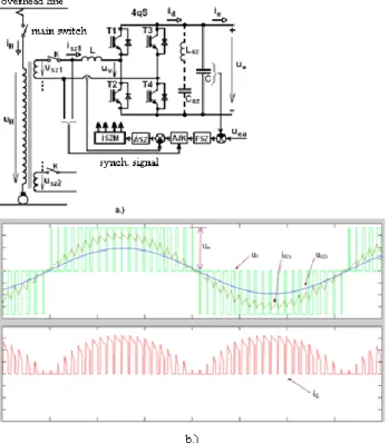
![Figure 3-5.: Simulated results of 4qS voltage and current time functions (brown: u sz1 [V], blue: i sz1 [A], green:](https://thumb-eu.123doks.com/thumbv2/9dokorg/1116499.78222/29.892.107.748.180.516/figure-simulated-results-voltage-current-functions-brown-green.webp)

![theothervehiclesarealsoinmotion,thehandlingofintersectionscenariosisacomplex inthearchitectureofthecontrolsystemitcanbehandledasaspecialfeatureofapath , ].Nevertheless,consideringpositionerrorscausedbyhumanparticipants,robustcontrol ]andGPSandstereovision](data:image/gif;base64,R0lGODlhAQABAIAAAP///wAAACH5BAEAAAAALAAAAAABAAEAAAICRAEAOw==)