Article
The Design of Performance Guaranteed Autonomous Vehicle Control for Optimal Motion in Unsignalized Intersections
Balázs Németh1,2,* and Péter Gáspár1
Citation: Németh, B.; Gáspár, P. The Design of Performance Guaranteed Autonomous Vehicle Control for Optimal Motion in Unsignalized Intersections.Appl. Sci.2021,11, 3464. https://doi.org/10.3390/
app11083464
Academic Editor: Luigi Fortuna
Received: 26 February 2021 Accepted: 6 April 2021 Published: 13 April 2021
Publisher’s Note:MDPI stays neutral with regard to jurisdictional claims in published maps and institutional affil- iations.
Copyright: © 2021 by the authors.
Licensee MDPI, Basel, Switzerland.
This article is an open access article distributed under the terms and conditions of the Creative Commons Attribution (CC BY) license (https://
creativecommons.org/licenses/by/
4.0/).
1 Institute for Computer Science and Control (SZTAKI), Eötvös Loránd Research Network (ELKH), 13-17. Kende utca, H-1111 Budapest, Hungary; peter.gaspar@sztaki.hu
2 Department of Control for Transportation and Vehicle Systems, Budapest University of Technology and Economics, 3-7. M ˝uegyetem rakpart, H-1111 Budapest, Hungary
* Correspondence: balazs.nemeth@sztaki.hu or nemeth.balazs@kjk.bme.hu
Abstract: The design of the motion of autonomous vehicles in non-signalized intersections with the consideration of multiple criteria and safety constraints is a challenging problem with several tasks. In this paper, a learning-based control solution with guarantees for collision avoidance is proposed. The design problem is formed in a novel way through the division of the control problem, which leads to reduced complexity for achieving real-time computation. First, an environment model for the intersection was created based on a constrained quadratic optimization, with which guarantees on collision avoidance can be provided. A robust cruise controller for the autonomous vehicle was also designed. Second, the environment model was used in the training process, which was based on a reinforcement learning method. The goal of the training was to improve the economy of autonomous vehicles, while guaranteeing collision avoidance. The effectiveness of the method is presented through simulation examples in non-signalized intersection scenarios with varying numbers of vehicles.
Keywords:coordinated control design; autonomous vehicles; learning-based control
1. Introduction and Motivation
The handling of intersection scenarios is an important challenge in the research field of autonomous vehicles. From the aspect of control design, several crucial tasks of the autonomous vehicle control in intersection scenarios should be formulated. For example, the ordering of autonomous vehicles in intersections has an impact on the energy consumption of the vehicles, traveling time, emissions and traveling comfort (due to the acceleration/deceleration maneuvers, for example) [1]. This leads to a multi-objective optimization task, which generally has a Pareto-optimal solution. Moreover, the solution of the optimization problem regarding autonomous vehicles in intersections can require lengthy computations. This poses the challenge of the minimization of the computational time, e.g., finding approximations of the optimal solution. From an application point of view, the accurate detection of a vehicle’s position in an intersection can be difficult. There exist camera-based vehicle localization strategies [2], solutions with LiDAR and camera fusion [3] and GPS and stereovision-based visual odometry solutions [4]. The detection and prediction of human behavior are also difficult and complex problems; see [5,6].
Nevertheless, considering position errors caused by human participants, robust control strategies are needed with which collision avoidance can be guaranteed.
Due to the special challenges of the control of autonomous vehicles in intersections, in the architecture of the control system it can be handled as a special feature of a path planning algorithm in future vehicles. Its main differences from the path planning problem are as follows. First, in intersections the autonomous vehicles can have interactions. Since the other vehicles are also in motion, the handling of intersection scenarios is a complex problem, which requires sensing, decision and control functionalities. In intersections the
Appl. Sci.2021,11, 3464. https://doi.org/10.3390/app11083464 https://www.mdpi.com/journal/applsci
risk of the collision is increased, e.g., compared to the motion of the autonomous vehicle along a highway. Second, various types of intersections on the road can be found—they can depend on the number of lanes, directions and signalization. A challenge of the autonomous vehicles and the intelligent transportation systems is the handling of vehicle interactions in unsignalized intersections [7]. In these types of intersections, the experiences of the human drivers has a role in the avoidance of the conflicts; e.g., the speed of the surrounding vehicles and the intentions of the further drivers must be estimated. In a general path planning algorithm, the waypoints, the rules and the information on the road and on the local traffic conditions can be considered to be given, and thus, it requires less estimation. Third, in urban areas the autonomous vehicles during their routes must travel through many intersections. Since these intersections are connected to each other, the motion of the vehicles in the intersections has an impact on the global performance of the traffic system, i.e., on the average speed or on the traffic density; see, e.g., [8].
Thus, during the design of the autonomous vehicle’s motion, the time minimization is an especially important at intersections. Moreover, the inefficient motion of autonomous vehicles in intersections can lead to increased energy consumption, e.g., a high number of stop and go maneuvers. Thus, during the design of the autonomous vehicle motion in intersections, a balance between the time minimization and the energy consumption minimization must be found. Although it is also a problem in a general path planning problem, it is a greater problem for intersections. Fourth, a special problem of vehicle control in intersections is the architecture of the control system. Since in intersections a high number of vehicles can be controlled and the presence of human-driven vehicles must be handled, an optimal solution of the motion problem can be found through the coordination of the autonomous vehicles in a centralized control system [9]. Nevertheless, it can require centralized control, which can lead to additional security, legal and privacy problems.
Therefore, it is requested to develop distributed control structures; e.g., in [10] the problem is formulated as distributed optimal control for a system of multiple autonomous vehicles and then solved using a nonlinear model predictive control (MPC) technique. Similarly, Kloock et al. [11] investigated intersection control of multiple vehicles using a distributed MPC approach, where priorities need to be assigned to vehicles. Thus, the challenge of distributed control is also different to the general path planning and tracking problems, where the coordination of the vehicles is limited, or where it is carried out on the level of the transportation system.
The high number of challenges in the field of autonomous vehicle control in inter- sections has motivated increased research activity, i.e., several publications with different approaches. Methods of one of the most important groups are based on the MPC technique;
see, e.g., [12–15]. Although they can provide appropriate results, the increase in the number of vehicles can make real-time computation difficult. A possible solution to the problem of increasing computational effort is the approximation of the optimal solution with neural networks; see, e.g., [16]. However, in this case it may be difficult to provide guarantees on collision avoidance for all intersection scenarios [17]. The quadratic programming method gives the possibility of real-time implementation compared to the convex optimization using space coordinates; see [18]. Collision avoidance is guaranteed through the definition of regions in the intersection with special rules, which reduces the complexity of the prob- lem, but the conservativeness of the solution increases. Due to the ordering problem of vehicles in an intersection, the control problem can be formed as a mixed-integer linear programming (MILP) task; see, e.g., a method on the coordination in [19]. The goal of the control is to find an arrival schedule of the vehicles, which ensures safety while it reduces the number of stops and intersection delays. Muller et al. [20] presents a cen- tralized MILP-based approach for intersection control in an urban environment of highly automated vehicles, with which the minimum vehicle delay at the intersection can be achieved. Another solution in the predictive control framework is to examine all ordering combinations of the vehicles [21], which can also be difficult for a high number of vehicles.
Thus, although MPC-based methods can provide effective and handy solutions to the
control problem of autonomous vehicles in intersections, a high number of vehicles can lead to numerical difficulties.
A further group of solutions is based on the minimax formulations of the optimal control problem, together with the coordination of the vehicles. For example, Tian et al. [22] proposed a game-theoretic approach to modeling vehicle interactions, in particular, for urban traffic environments with unsignalized intersections. In general, they are traffic models with heterogeneous control, and they are used for virtual testing, evaluation and calibration of autonomous vehicle control systems. A framework for intersection control, which is based on the queuing theory, was presented by [23]. Through this framework a capacity-optimal, slot-based intersection management system for the two- road crossing configuration was presented. A slot preassigning method for connected vehicles was also proposed in [24]. The connection of intersections can also be handled by the multi-agent viewpoint [25,26]. This solution provides the ability to quickly reverse individual lanes in response to rapidly changing traffic conditions. A further multi-agent solution based on a heuristic optimization algorithm was presented by [27]. The objective of the research was to reduce total time delay for the entire intersection, while collisions were prevented. The approaches in the field of trajectory planning are possible ways to formulate the problem of autonomous vehicle motion in intersections. The actual methods and the future challenges in path planning are summarized in [28]. Some similarities between the path planning and the problem of autonomous vehicles in intersections motivated the use of Bézier-based methods in the problem. For example, in [29] a Bézier curve optimization method was proposed to cope with these constraints, and autonomous vehicles were considered that were equipped with all the necessary sensors for obstacle detection. In this way, the obstacle avoidance problem was transformed into an optimization problem under equality constraints. Another method with the use of Bézier curves was found in [30], which presents a novel method to resolve the obstacle avoidance and overtaking problems named Hybrid Planning. An MPC-based solution to track the lane centerline while avoiding collisions with obstacles was found in [31]. Further relevant works in the topic of path planning are as follows. Hu et al. [32] presented a real-time dynamic path planning method; i.e., an optimal path with appropriate acceleration and velocity profiles is the result. A graph-based planning method to generate an actionable set of multiple drivable trajectories for race vehicles, is found in [33]. For road vehicles, Werling et al. [34] proposed an optimal trajectory generation method, with which velocity maintenance, merging, following, stopping and a reactive collision avoidance functionality were achieved. In [35]
a real-time safe stop trajectory planning algorithm, based on selection from a precomputed set of trajectories has been developed. Several papers deal with the selection of the velocity of autonomous vehicles, which has relevance in the problem of intersection scenarios.
For example, Herrmann et al. [36] proposed an optimization-based velocity planner using the multi-parametric sequential quadratic problem, with which a spatially and temporally varying friction coefficient, and a race-focused energy strategy for the road can be handled.
In [37] a solution to the mathematical problem behind the trajectory design problems has been provided; i.e., a general-purpose solver for convex quadratic programs based on the alternating direction method of multipliers is proposed. Moreover, in [38] a real-time velocity optimization algorithm for fixed paths was developed and implemented.
Another important group of efficient solutions on the problem contains the learning- based approaches, especially reinforcement learning (RL) [39–42]. The advantage of this method is its model-free property, which can provide solutions to the problem of constraint formulation. Moreover, the training of the control agent through a high number of epochs is carried out, which can lead to improved performances. A deep RL method was applied to unsignaled intersections in [39]. It also provided an analysis to explore the ability of the system to learn active sensing behaviors and safe navigation in the case of occlusions.
Tran and Bae [43] also presented a deep RL-based model that considers the effectiveness of leading autonomous vehicles in mixed-autonomy traffic at a non-signalized intersection.
Yudin et al. [44] offered a new approach to training the intelligent agent that simulates
the behavior of an unmanned vehicle, based on the integration of reinforcement learning and computer vision. Using full visual information about the road intersection obtained from aerial photographs, they studied through automatic detection the relative positions of all road agents with various architectures of deep neural networks. In spite of promising achievements, the resulting neural-network-based agents cannot provide a guarantee of collision avoidance for the vehicles.
That short review of the existing literature showed that several efficient solutions exist, but there are challenges for achieving a reliable control method. The goal of the recent research activities was to find a control design method with which many autonomous vehi- cles can be handled, while the energy consumption and time minimization requirements, along with safety, i.e., the avoidance of collisions, are ensured. Similarly, the purpose of this paper is to provide a novel solution to the recent problems through the following concept. The increase in the number of vehicles is handled through separation, i.e., the control designed for individual autonomous vehicles, which considers limited information on the environment. In the solution the performance requirements are priorized and the specifications are guaranteed through different methods, such as optimal control and RL-based techniques. Thus, in this way the advantages of each method, such as providing guarantees and optimization of the performance level, can be achieved.
This paper focuses on the optimal design of the longitudinal control of an autonomous vehicle. Its elements and the related problems regarding the paper can be summarized as follows.
• The objective may contain multiple criteria, the most important of which are the minimization of traveling time, energy consumption and the maximization of com- fort. The variables of the optimization task are the control inputs of the vehicles, e.g., longitudinal acceleration commands or traction/braking forces.
• The dynamics of each vehicle provide constraints in the optimization problem.
• Furthermore, the safe motion of the vehicles, i.e., collision avoidance, must be guaran- teed, which leads to constraints for vehicles with intersecting routes.
• The velocity of the vehicles must be kept in a predefined range, considering the speed limit.
• The control input of the vehicles must also be limited due to the physical limits of the driveline, the braking system and the tire–road contact.
In this paper the optimization problem of the vehicle’s motion is divided according to the performance aspects. First, a quadratic optimization problem is proposed, whose role is to guarantee collision avoidance and the limitation of the velocities of vehicles. The con- straint of collision avoidance is formed through a linear approximation of the quadratic constraint, which leads to high efficiency in computation. The quadratic optimization is solved at every time step during the motion of the vehicles. Second, the advantages of reinforcement learning in the improvement of the economy performances, e.g., the minimization of the control input, are exploited. In the training process the previously formed quadratic optimization task is applied as a part of the environment for learning.
Similarly, during the operation of the control system, the trained neural network and the quadratic optimization task operate together. The effectiveness of the resulting control system through simulation examples with various vehicles is analyzed.
Thus, the contributions of the paper are as follows. The control design problem for autonomous vehicles in intersections is formed in a novel way through the division of the problem. It leads to the reduced complexity of the control problem in real-time computation.
Moreover, an environment model for reinforcement learning is created, which guarantees that collision avoidance can be provided. An important benefit of the method is that the safety performance level of the resulting control structure is guaranteed; i.e., a collision of vehicles cannot be caused by the learning-based control agent. From an application point of view, an advantage of the method is that it is able to handle various situations at the intersection; i.e., the method is independent of the number of vehicles. Although this paper focuses on autonomous vehicle control, the proposed control design method may be used
for further applications, considering the similarities with the intersections. For example, in the field of microfluid research, an actual problem is to find modeling and control methods for the handling of T-junctions [45]. In [46] computational models for microfluidic bubble logic systems with T-junctions have been proposed. Learning methods have also been used for control purposes in this context; see, e.g., [47]. Thus, the contributions of the proposed control system may have relevance to further applications.
The paper is organized as follows. In Section2the model formulation for handling intersection scenarios is proposed. The cruise control design for the autonomous vehicle with robustness issues is found in Section3. The application of reinforcement learning for the improvement of economy performances is presented in Section4. In Section5 the effectiveness of the proposed method is shown through simulation examples. Finally, the conclusions and the future challenges are provided in Section6.
2. Model Formulation for Handling Intersection Scenarios
The goal of this section is to formulate the collision-free motion of the vehicles in intersection scenarios. The formulation includes the longitudinal motion model of the vehicles and the constraints on their motion to avoid collisions.
The longitudinal motion of the vehicles is formulated through the simplified kinemat- ics of vehicles:
vi(k+1) =vi(k) +Tai(k), (1) si(k+1) =si(k) +Tvi(k) + T
2
2 ai(k), (2)
whereiindex represents the id of the vehicle,nis the number of vehicles,viis longitudinal velocity andsiis longitudinal displacement.airepresents the longitudinal acceleration of the vehicle, which is handled as a control input command, andTis the time step of the discrete motion model. The longitudinal displacement is related to the center point of the intersection, and thus, it is defined assi =0 for alliat the center point. The longitudinal displacement of the approaching vehicle has a negative value, and the displacement of the vehicle moving away has a positive value.
In the environment model of the intersection, the autonomous ego vehicle is numbered 1. Thus, for example, in the case ofn =5 in the environment, the ego vehicle and four surrounding vehicles are incorporated. The control input of the autonomous vehicles is separated into two elements, as has been introduced in Section1as
a1(k) =aK(k) +∆(k), (3) whereaKis the control input command of the robust longitudinal controller and∆(k)is the additional input from the supervisor in the model.
The purpose of the supervisor in the collision-free motion model is to select∆(k)for the autonomous ego vehicle with the following objectives and constraints.
• The objective of the selection is to minimize the difference between the current control inputa1(k) and the output of the learning-based controlleraL(k). The aim of the minimization is to preserve the performance level of the learning-based controller, if possible.
• Some of the vehicles can intersect their routes at the intersection. Thus, an interven- tion witha1(k)must provide motion for the autonomous vehicle, with which a safe distancessa f ebetween the autonomous vehicle and the other surrounding vehicles with intersecting routes can be guaranteed. Since the number of vehiclesncan be high, a limited amount of surrounding vehicle motion must be simultaneously consid- ered; i.e.,nsrepresents the number of vehicles which are incorporated into the design process. It is a constraint in the selection of∆.
• The velocity of the vehicles must be inside of a predefined range. The upper bound of the range is defined by the speed limitvmaxor the curvature of the intersection.
The lower bound is represented by the stopping of the vehicle. Thus, it is necessary to select∆for all vehicles to keep velocities inside of the range. It is also a constraint in the selection process.
The selection process of∆for the autonomous ego vehicle is formed as an optimization problem as follows:
min∆(k) a1(k)−aL(k)2 (4a) subject to
(s1(k+1)−sj(k+1))2≥ssa f e, ∀j∈ns, (4b)
0≤v1(k+1)≤vmax, (4c)
∆∈∆, (4d)
where jrepresents the surrounding vehicles, whose motion can be in conflict with the autonomous vehicle; i.e., their routes are intersected. ∆represents the domain of the optimization variable. In the optimization problem the kinematics of the vehicle motion (1) is considered through the formulation of the constraints, the separation of the control input (3) is involved in the objective function.
The objective (4a) is transformed using (3) as
a1(k)−aL(k)2= aK(k) +∆(k)−aL(k)2=∆(k)2+2f(k)∆(k) + (aK(k)2+aL(k)2−2aL(k)aK(k)), (5) where f(a vector) is formed as f(k) =aK(k)−aL(k). Since(aK(k)2+aL(k)2−2aL(k)aK(k)) is independent of∆(k), it is omitted in the rest of the optimization problem.
The constraint for collision avoidance (4b) is formed to keepssa f ebetween the vehicles.
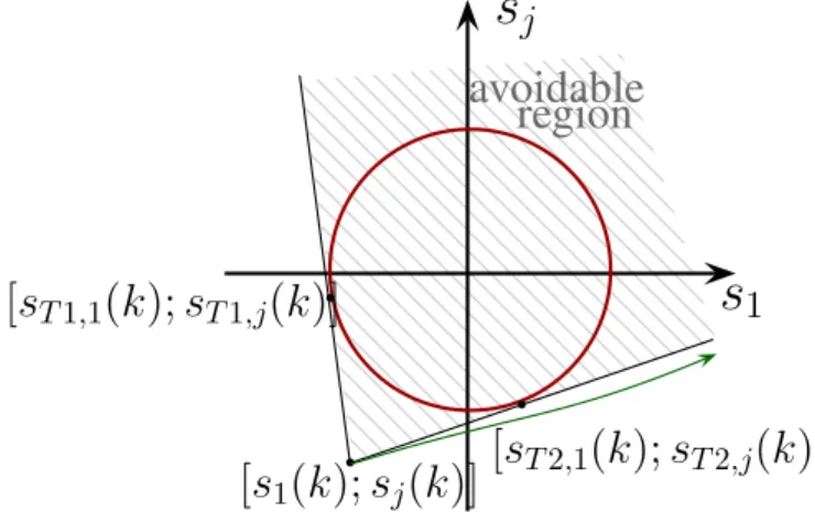
The distance is measured in the sense of the longitudinal displacements of the vehicles on their routes. Geometrically, the quadratic constraints (4b) represent that the trajectories of the autonomous vehicles1and the related surrounding vehicles must be out of a circle.
The radius of the circle is defined byssa f e; see Figure1a. For example, it there are two surrounding vehicles and the autonomous vehicle the trajectories must be out of a sphere, whose radius is represented byssa f e; see Figure1b.
s
1s
js
saf e[s
1(k); s
j(k)]
avoidable region
(a)Constraint illustration of a related pair
s1
sj
sl
[s1(k);sj(k);sl(k)]
ssaf e
(b)Constraint illustration on an example Figure 1.Geometrical illustration of the quadratic constraints.
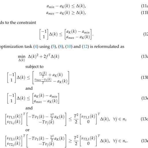
Although the circle perfectly describes the region of = state-space that must be avoided, it leads to a quadratic constraint in the optimization problem (4). Since the optimization problem must be solved at eachktime step during the motion of the vehicles, the quadratic constraint can make the solution of the optimization more complex, and it can make
the real-time solution more difficult. This motivates the transformation of the quadratic constraints into linear constraints. In this paper it is performed through the approximation of the avoidable regions of circles to the avoidable regions of half-planes.
The method of the approximation is illustrated in Figure2. First, the tangent lines to the circle from the actual state
s1(k) sj(k)Tare assigned. The avoidable half-plane is determined by the region between the tangent lines; i.e., the trajectories must be out of it.
Second, two linear inequality constraints are specified, which represent that the trajectory of the state must be out of the avoidable half-plane:
sT1,1(k) sT1,j(k)
T s1(k) sj(k)
≤
sT1,1(k) sT1,j(k)
T
s1(k+1) sj(k+1)
, (6a)
or sT2,1(k)
sT2,j(k) T
s1(k) sj(k)
≥
sT2,1(k) sT2,j(k)
T
s1(k+1) sj(k+1)
, (6b)
where
sT1,1(k) sT1,j(k),
sT2,1(k) sT2,j(k)are the tangent points on the circle at time stepk. Note that the linear constraints result in an outer approximation of the avoidable set.
There are regions of the half-space which cannot be reached due to the linear constraints, but they are out of the circle.
s j
s 1
[s
1(k); s
j(k)]
[s
T1,1(k); s
T1,j(k)]
[s
T2,1(k); s
T2,j(k)]
avoidable region
s j
Figure 2.Illustration of constraint approximation.
The longitudinal displacement of the autonomous vehicle atk+1 in (6) is transformed to express the linear constraints in terms of∆. The transformation is based on the mo- tion equation (1) and the relation of actuation separation (3). Moreover, the motions of surrounding vehicles fork+1 with their actual velocityvj(k)are predicted this way:
s1(k+1) =s1(k) +Tv1(k) + T
2
2 aK(k) +T
2
2 ∆(k), (7a)
sj(k+1) =sj(k) +Tvj(k), (7b) which can be substituted into (6). It leads to the linear constraints
sT1,1(k) sT1,j(k)
T"
−Tv1(k)−T22aK(k)
−Tvj(k)
#
≤ T
2
2
sT1,1(k) 0
T
∆(k), (8a) or
sT2,1(k) sT2,j(k)
T"
−Tv1(k)−T22aK(k)
−Tvj(k)
#
≥ T2 2
sT2,1(k) 0
T
∆(k). (8b)
Figure2illustrates that the reachable set for the state
s1(k+1) sj(k+1)Tis non-convex, which means that (8) formulates disjunctive inequalities. However, each constraint in (8) leads to convex reachable sets, which means that the optimization problem can be divided, as it is proposed below.
Another constraint in the optimization (4) is on the velocity of the autonomous vehicle;
see (4c). In the case of this constraint,vi(k+1)is expressed in terms of∆using the motion equation (1) and the relation of actuation division (3). The linear inequality constraint is formed as
0≤v1(k) +TaK(k) +T∆(k), , (9a) vmax ≥v1(k) +TaK(k) +T∆(k), (9b) which leads to
−1 1
∆(k)≤
" v
1(k)
T +aK(k)
vmax−v1(k)
T −aK(k)
#
, (10)
wherevmaxis the maximum velocity of the autonomous vehicle. In an urban environment it is determined by the velocity regulations, and in the case of cornering maneuvers at intersections, the curvature avoids skidding.
The last constraint in the optimization problem (4) is the limitation of the resulting optimization variable; see (4d). The value of∆is limited by the bounds ofa1(k), such as aminandamax, which represent full braking and throttle. Sincea1(k)is also influenced by aK(k), the constraints on∆(k)are formed as
amin−aK(k)≤∆(k), (11a)
amax−aK(k)≥∆(k), (11b)
which leads to the constraint −1
1
∆(k)≤
aK(k)−amin
amax−aK(k)
. (12)
The optimization task (4) using (5), (8), (10) and (12) is reformulated as
min∆(k) ∆(k)2+2fT∆(k) (13a)
subject to −1
1
∆(k)≤
" v
1(k)
T +aK(k)
vmax−v1(k)
T −aK(k)
#
(13b) and
−1 1
∆(k)≤
aK(k)−amin
amax−aK(k)
(13c) and
sT1,1(k) sT1,j(k)
T"
−Tv1(k)−T22aK(k)
−Tvj(k)
#
≤ T
2
2
sT1,1(k) 0
T
∆(k), ∀j∈ns (13d) or
sT2,1(k) sT2,j(k)
T"
−Tv1(k)−T22aK(k)
−Tvj(k)
#
≥ T2 2
sT2,1(k) 0
T
∆(k), ∀j∈ns. (13e)
The quadratic optimization in (13) contains disjunctive inequalities. This means that the optimization task for the solution can be reformulated to a mixed-integer optimization
problem [48]. In practice, the optimization problem (13) can be solved as a set of quadratic optimization problems, which has only “and” conditions between the constraints. Thus, in the case ofnssurrounding vehicles, 2ns distinct constrained optimization problems can be formed. Since the objective function for each problem is the same, the global minimum solution can be found through a comparison of their solutions. Finally, the solution is yielded by∆(k), which leads to the minimum value of the objective function, considering all of the optimization tasks. The optimization problem during the motion of the autonomous vehicle is continuously solved.
3. The Design of Robust Cruise Control
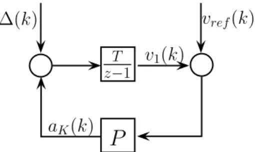
An intervention in the longitudinal dynamics of the autonomous vehicle at an inter- section has great importance for achieving the required motion profile for time stepk+1.
The control input of the vehicle is composed by two elements, aK(k)and∆(k); see (3).
The computation of∆(k)in Section2has already been proposed. In this section the design of the control interventionaK(k)is proposed.
The most important requirements for the controller are formed as follows.
• The control system must guarantee safe longitudinal motion for the vehicle, even ifaL
has degradation or a fault scenario. The safe motion is guaranteed throughaKand∆.
• The longitudinal controller must have robust characteristics, becausea(k)6=aK(k), if∆(k)6=0. Robustness must also be guaranteed in extreme vehicle dynamic scenarios:
for example, ifaK(k)suggests full throttle, but it has been overridden by∆(k)to be full braking. Similarly, robustness must be guaranteed ifaK(k)suggests full braking, but it has been overridden by∆(k)to be full throttle.
• The control signal aK(k)must be computed to avoid the saturation of the control actuationa(k). Since in the computation process the computation ofaK(k)is prior to
∆(k), the result of (13) is not considered in the computation ofaK(k). Thus, the role of the cruise controller is to guaranteeamin≤aK(k)≤amax.
The design of the longitudinal controller is based on the simplified vehicle model (1) with one state, such as the longitudinal velocityv1(k). The controller is formed as a gainP for velocity tracking, whose input is the velocity error; see Figure3. The reference signal for the tracking isvre f. The idea behind the formulation of the control design as a tracking problem is as follows. The vehicle must adapt to the environment, which determines the achievable velocity of the vehicle, e.g., through maximum speed limits. The aim of the cruise control is to consider the regulations and the motion of the other vehicles to achieve safe motion. The maximum speed limit information is provided byvre f(k), and information on the motion of the vehicles in the environment in the computation of∆(k)is included. Thus, through the selections ofvre f(k)and∆(k), safe motion is guaranteed.
P
v
ref(k)
∆(k)
T z−1
v
1(k )
a
K(k)
Figure 3.Closed-loop structure of the longitudinal control.
The selection ofPis determined by the requirement of robustness by the controlled system. In the presented structure,∆(k)is handled as a disturbance and the performance of the system is the minimization of the tracking error, such as|vre f(k)−v1(k)|. Thus, for the robustness issue, it is necessary to limit the impact of∆(k)disturbance on the performance.
The robustness criterion is based on the small-gain theorem [49]. As a consequence, theH∞
norm transfer function from ∆(k)on the velocity error must be smaller than 1, which guarantees disturbance attenuation.
In the computation of the transfer function the maximum value of the ¯∆=|∆(k)|is also considered. The maximum is determined by the vehicle dynamic scenario, if∆(k) implies full throttle instead of full braking or full braking is implied instead of full throttle.
Thus, the value of ¯∆is|amin|+|amax|. The transfer function from ∆i(k)to the velocity error is
G(z) = ∆¯
T z−1
1+zP−·T1. (14)
The criterion on the selection ofPis to guarantee||G(z)||∞<1.
The constraint on the control inputa1(k)is influenced by the limitation of the ref- erence signal. The reference velocity in Figure3represents the maximum speed limit vmax(k)for the vehicle on the given road section. Nevertheless, it is necessary to provide a reference velocity for the vehicle, with which the constraint ona(k)is kept. Thus,vre f(k)is computed as
vre f(k) =v1(k) +min amax
P , max amin
P ,vmax−v1(k)
. (15)
The expression represents that the reference velocity can differ from that actual velocity with a limited value. The value ofPhas a role in the computation of the reference signal.
Finally, the method of the selection ofPis as follows. It is recommended to select a value ofPas high as possible, which can result in fast operation of the tracking control.
However, the value ofPis constrained by the robustness criterion:
max P, (16a)
subject to
||G(z)||∞<1. (16b)
The output of the robust longitudinal controller isaK(k), which is used in the compu- tation of the control input (3) and in the computation of∆(k)(13).
4. Design of Motion Profile Using Reinforcement Learning
In the previous sections a control strategy was formed with which the safe motion of the autonomous vehicle in an intersection can be guaranteed. Nevertheless, in the design problem of the vehicle motion there are economy aspects that should be considered during the design process; i.e., it is recommended to minimize the control energy of the vehicles. In this section the consideration of the economy performance in the design process is proposed.
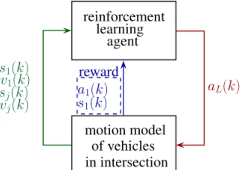
The goal of the design process is to find an agent which is able to generate the control signalaL(k). The agent is trained through a reinforcement learning process. The structure of the design process is illustrated in Figure4. The model for the learning process contains the optimization task (13) together with the result of the robust control design (16). The model guarantees the avoidance of the collision in the intersection for everyaL(k)signal. Thus, during the training process of the agent in every episode the safety performances are guaranteed, and similarly, the economy performance is improved. The output of the motion model is rewardr(k), which is composed bya(k)andv1(k)as follows:
r(k) =−Q1a2i(k) +Q2(s1(k)−s1(0)), (17) whereQ1andQ2positive values are design parameters, which scale the importance of each term inr(k). The reward contains the control inputs in the vehiclesa(k), which represent the economy performance of the vehicles. If the reward contains onlya(k), it can result
in unacceptably slow motion for the autonomous vehicle, becausea(k) = 0 is the best choice for the maximization of the reward. Thus, in the reward the traveled distance of the autonomous vehicle(s1(k)−s1(0))is also incorporated, wheres1(0)is the initial position of the autonomous vehicle. The observation for the agent includes the position of the autonomous vehicless1(k)and of the surrounding vehiclessj(k)j∈ns, and their velocities v1(k),vj(k)j∈ns.
in intersection motion model
of vehicles reinforcement
learning agent
aL(k) a1(k)
s1(k) reward s1(k)
v1(k) sj(k) vj(k)
Figure 4.Control structure in the learning process.
The goal of the reinforcement learning process is to maximize reward (17) during episodes. In this paper the training process through the deep deterministic policy gradient (DDPG) is carried out, which is a model-free, online, off-policy reinforcement learning method [50]. A DDPG agent is an actor-critic reinforcement learning agent that computes an optimal policy that maximizes the long-term reward. In this method, actor and critic approximators are used. Both approximators use the observations, which are represented byS. The purpose of the actor approximatorµ(S)is to find the actionAwithaL(k), which maximizes the long-term future reward. The role of the criticQ(S,A)is to find the expected value of the long-term future reward for the task.
The result of the training process is an agent whose output isaL(k). In the control process of the autonomous vehicle, the agent works together with the control strategy (13).
As a result, the collision avoidance of the vehicles in the intersection is guaranteed, and similarly, the economic performance of the vehicles is improved.
5. Simulation Results
Four simulation examples are shown to illustrate the effectiveness of the designed controller. The first and second examples show simplified scenarios, in which three vehicles are at the intersection. The goal of the simulations in scenario 3 is to shown that the proposed control system is able to adapt to various traffic environments, depending on the initial velocities and positions of the vehicles. The fourth example has increased complexity, in which seven vehicles are incorporated. In these simulations the closest three vehicles in the constraints of the optimization tasks are incorporated.
The RL-based agent was trained through 500 simulation scenarios, in which the number of vehicles, their initial velocities and positions were selected randomly; i.e., the vehicle number was varied between 1 and 7, the initial positions were selected between
−20 m . . .−40 m and the initial velocities were varied between 10 km/h . . . 50 km/h.
In the learning process of the neural networks, the following structures have been trained.
The actor network had eight neurons in the input layer; three fully connected layers with 48 neurons and Rectified Linear Unit (ReLU) functions in each layer; and one neuron with hyperbolic tangent functions in the output layer. The critical network has the same structure. In the structure and parameter selection of the neural networks, the k-fold cross-validation technique [51] and a hidden-layer number optimization process [52] can be used. The sampling time in each episode is selected atT =0.05 s. The terms in the reward function are considered with the same design parameters, such asQ1=−0.1 and
Q2=10. The training process has been performed through Matlab 2020a Reinforcement Learning Toolbox [53] on an Intel i7 CPU.
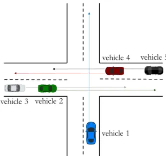
For the simplified examples, the first and second scenarios are illustrated in Figure5.
In these cases, vehicle 1 is the ego vehicle; vehicle 2 and vehicle 3 are the surrounding vehicles on the perpendicular road section. Both surrounding vehicles cross the route of vehicle 1, which results in a conflict situation. In the first scenario the following initial conditions were set: s1= −40 m,s2= −36 m,s3 = −41 m and all of the vehicles have 50 km/h initial velocity. In the second scenario, vehicle 3 had different settings, while the other vehicles had the same initial conditions, i.e.,s2=−48 m andv2=30 km/h. The safe distance was set tossa f e =8 m.
Figure 5.Illustration of the simplified intersection scenarios.
The results of the simplified scenarios are found in Figure6. Figure6a,b shows that the autonomous ego vehicle is able to guarantee keepingssa f e. Nevertheless, in the two scenarios, the ordering of the vehicles in the intersection is different. Since in scenario 1 the surrounding vehicles have increased velocity, the autonomous vehicle decides to reduce its velocity to 18 km/h and allows the surrounding vehicles with right of way to enter the intersection. In scenario 2 the autonomous vehicle has enough time to go through the intersection before vehicle 3 enters it. Thus, in this casev1can be increased after vehicle 2 leaves the intersection, see Figure6d. The differences in the motion of vehicle 1 also influence the trajectories in Figure6a,b. Moreover, the control input signals for each scenario are found in Figure6e,f. In case of scenario 2 the acceleration of the ego vehicle is increased to 3 m/s2in 2.6 s to avoid a collision with vehicle 2, while in scenario 1 the acceleration is increased later than 3 s by a lower value.
-40 -30 -20 -10 0 10 20 30 40 s1 (m)
-30 -20 -10 0 10 20 30
s2,3 (m)
avoidable region s1-s2 s1-s3
(a)Trajectories of the vehicles in scenario 1
-40 -30 -20 -10 0 10 20 30 40
s1 (m) -30
-20 -10 0 10 20 30
s2,3 (m)
avoidable region s1-s2 s1-s3
(b)Trajectories of the vehicles in scenario 2
0 1 2 3 4 5 6
Time (s) 15
20 25 30 35 40 45 50
Velocity (km/h)
(c)Velocity in scenario 1
0 1 2 3 4 5 6
Time (s) 20
25 30 35 40 45 50
Velocity (km/h)
(d)Velocity in scenario 2
0 1 2 3 4 5 6
Time (s) -4
-3 -2 -1 0 1 2 3
a (m/s2)
(e)Control input in scenario 1
0 1 2 3 4 5 6
Time (s) -4
-3 -2 -1 0 1 2 3
a (m/s2)
(f)Control input in scenario 2 Figure 6.Signals of the simplified scenarios.
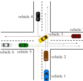
In the next simulation examples, it is proposed that the proposed algorithm provides safe motion for the autonomous vehicle in various scenarios. The intersection scenario is illustrated in Figure7, where vehicle 1 represents the autonomous vehicle and the other vehicles are the surrounding vehicles. In the next four simulations the initial positions and velocity values of the vehicles are varied, and thus, a varying ordering in the intersection is yielded. In all of the simulations, vehicle 1 has conflicts with the surrounding vehicles because of their route crossing. The goal of the simulations are to show that the autonomous vehicle is able to adapt to various traffic scenarios, and the proposed optimization (13) together with the reinforcement learning is efficient. The initial position and velocity values of the scenarios are listed in Table1.
Figure 7.Illustration on the intersection scenario with 5 vehicles.
Table 1.Initial conditions for scenario 3.
Initial Condition Scenario 3a Scenario 3b Scenario 3c Scenario 3d
s1(0) −8 m −25 m −26 m −30 m
s2(0) −20 m −10 m −20 m −10 m
s3(0) −30 m −30 m −8 m −25 m
s4(0) −25 m −8 m −25 m −8 m
s5(0) −35 m −35 m −45 m −30 m
v1(0) 50 km/h 50 km/h 40 km/h 35 km/h
v2(0) 50 km/h 50 km/h 50 km/h 50 km/h
v3(0) 35 km/h 35 km/h 50 km/h 50 km/h
v4(0) 50 km/h 50 km/h 50 km/h 50 km/h
v5(0) 45 km/h 45 km/h 40 km/h 45 km/h
Figure8shows the results of each scenario in the third simulation setup, related to Figure7. Figure8a illustrates the trajectories of scenario 3a, where vehicle 1 could go through the intersections first. Thus, the velocity of vehicle 1 was set to the constant maxi- mum 50 km/h, with which the avoidance of the collision was guaranteed; see Figure8b and the related control inputs in Figure8c. In scenario 3b the autonomous vehicle was further from the intersection at the beginning of the simulation; see Table1. Thus, it was not possible to go through the intersection first, and therefore, vehicle 1 was the third in line; see the trajectories in Figure8d.v1was slightly reduced before 2 s to guarantee the safe distance. Figure8f shows thatuwas close touLduring the entire simulation, which means that the learning process and the optimization (13) are efficient. In scenario 3c, the vehicle had reduced velocity related to the surrounding vehicles, and thus, it was fourth at the intersection (see Figure8g). While guaranteeing safe distance, the velocity was reduced, and at 5 s the the maximum velocity was achieved; see Figure8h. Althoughu is close touL, it is necessary to modify it to avoid the collision, e.g., between 1.5 s . . . 3.8 s (Figure8i). Figure8j shows the trajectories of scenario 3d, where vehicle 1 is the last in the ordering. Its reason is that the initial velocity is smaller than in scenario 3c; see Figure8k. Since for vehicle 5 the priority must be guaranteed, vehicle 1 must accelerate with a reduced value between 2 and 6 s; see the velocity profile in Figure8k and the acceleration command in Figure8l. Nevertheless,ucan be selected to be close touL, which can provide an improved level of economy performance, while the safety performance iis simultaneously guaranteed.
-30 -20 -10 0 10 20 30 40 50 s1 (m)
-30 -20 -10 0 10 20 30
s2,3,4,5 (m)
avoidable region s1-s2 s1-s3 s1-s4 s1s5
(a)Trajectories - scenario 3a
0 2 4 6 8 10
Time (s) 0
10 20 30 40 50
Velocity (km/h)
(b)Velocity - scenario 3a
0 2 4 6 8 10
Time (s) -1
-0.5 0 0.5 1
Control input (m/s2)
uL u uK
(c)Control input - scenario 3a
-30 -20 -10 0 10 20 30 40 50
s1 (m) -30
-20 -10 0 10 20 30
s2,3,4,5 (m)
avoidable region s1-s2 s1-s3 s1-s4 s1-s5
(d)Trajectories - scenario 3b
0 2 4 6 8 10
Time (s) 0
10 20 30 40 50
Velocity (km/h)
(e)Velocity - scenario 3b
0 2 4 6 8 10
Time (s) -3
-2 -1 0 1 2 3 4
Control input (m/s2)
uL u uK
(f)Control input - scenario 3b
-30 -20 -10 0 10 20 30 40 50
s1 (m) -30
-20 -10 0 10 20 30
s2,3,4,5 (m)
avoidable region s1-s3 s1-s2 s1-s4 s1-s5
(g)Trajectories - scenario 3c
0 2 4 6 8 10
Time (s) 0
10 20 30 40 50
Velocity (km/h)
(h)Velocity - scenario 3c
0 2 4 6 8 10
Time (s) -4
-3 -2 -1 0 1 2 3 4
Control input (m/s2)
uL u uK
(i)Control input - scenario 3c
-30 -20 -10 0 10 20 30 40 50
s1 (m) -30
-20 -10 0 10 20 30
s2,3,4,5 (m)
avoidable region s1-s2 s1-s3 s1-s4 s1-s5
(j)Trajectories - scenario 3d
0 2 4 6 8 10
Time (s) 0
10 20 30 40 50
Velocity (km/h)
(k)Velocity - scenario 3d
0 2 4 6 8 10
Time (s) -4
-3 -2 -1 0 1 2 3 4
Control input (m/s2)
uL u uK
(l)Control input - scenario 3d Figure 8.Signals of third scenarios.
Finally, the operation of the designed autonomous vehicle control system in a complex simulation scenario in urban context is analyzed. In the example, seven vehicles took part, i.e., the ego vehicle and six other surrounding vehicles. The illustration of the fourth scenario is found in Figure9. In this scenario the autonomous ego vehicle is illustrated as vehicle 1. In the example, all of the other vehicles are in conflict with vehicle 1, which means that the signals of vehicles 2–7 are used during the design of the control input a. The initial positions and velocity values are as follows: s1 = −34 m, s2=−25 m, s3=−4 m,s4=−30 m,s5=−75 m,s6=−102 m,s7=−128 m,v1=50 km/h,v2=50 km/h,v3 =40 km/h,v4 =50 km/h,v5= 50 km/h,v6= 40 km/h andv7=50 km/h.
In the scenario, ns = 3 surrounding vehicles during the solution of the optimization problem are considered.
Figure 9.Illustration on the complex intersection scenario.
Some scenes of scenario 4 can be found in Figure10. Moreover, the video of the entire scenario inhttps://youtu.be/VGqcoX-9YTYcan be seen. Figure10a shows that vehicle 2 and vehicle 3 already left the intersection and vehicle 4 was in the intersection performing a left turn. Since vehicles 2–4 were closer to the intersection than vehicle 1, the ego vehicle had to reduce its velocity to give way; see Figure11b. It was yielded by the actuation; see the acceleration commanduin Figure11c. Moreover, after vehicle 4 left the intersection, vehicle 5 arrived at 50 km/h; see Figure10b. Due to the reduced velocity of vehicle 1, it was not possible to go through between vehicle 4 and vehicle 5, and thus, vehicle 1 stopped.
Figure10c shows when vehicle 5 left the intersection, the velocity of vehicle 1 was increased to go through the intersection before vehicle 6 and vehicle 7 arrived (Figure10d).
(a)Vehicle 4 turns left (b)Vehicle 5 enters into the intersection
(c)Vehicle 1 starts to enter into the intersection (d)Vehicle 1 leaves the intersection Figure 10.Illustration of the complex fourth scenario.
Figure11 shows an insight into the operation of the control system. Figure 11a illustrates the trajectories of the vehicles and the avoidable region. The illustration shows that all of the trajectories are outside of the avoidable region, and thus, the safety constraint on the motion of the autonomous vehicle can be guaranteed. Figure11b shows the distances between vehicle 1 and the closest ns = 3 vehicles, where d1 is related to the distance between vehicle 1 and the closest vehicle andd3is related to the distance between vehicle 1 and the third closest vehicle. Note that the vehicles inns vary during the simulation, e.g., directly beforet=4 s distanced1is related tos1–s4,d2is relateds1–s5andd3is related tos1–s6; while directly aftert=4 s,d1is related tos1–s5,d2is relateds1–s6andd3is related tos1–s7. If there are less than three close vehicles, virtual vehicles with constant 100 m positions are defined; see, e.g.,d3after 5.5 s. Figure11b shows that all of the distances were abovessa f e=8 m during the entire simulation, independently from the selection of the closest vehicle. This was yielded by the control inputu, which is illustrated in Figure11d.
Figure11d also shows the further inputs, such asuK anduL. Since the role ofuKis to provide velocity tracking, its value was 3 m/s2constantly, becausev1<50 km/h during the entire simulation, except the initial velocity. The role ofuLis to provide vehicle motion, with which the reward function is maximized, so energy consumption is minimized and the traveled distance of the vehicle is maximized. However, none of the control inputs uKanduLare acceptable, because the safety constraints are not guaranteed. Thus,uKis modified through∆, which results in the control input signalu. The maximum deceleration of the vehicle before 5.5 s guaranteed the avoidance of collision with vehicles 2–5, and the maximum acceleration between 5.5 s . . . 8 s guaranteed the avoidance of the collision with vehicles 6 and 7. After 8 s, the conflict between the vehicles ceased, and thus, vehicle 1 could move withu=uLto minimize the objective in (13) to zero. As a result, the velocity of vehicle 1 was slightly increased after 8 s; see Figure11c. Moreover, Figure11c presents that the difference betweenvre f andv1is very small, which illustrates the effectiveness of the designed robust cruise control.
-30 -20 -10 0 10 20 30 40 50
s1 (m) -30
-20 -10 0 10 20 30
s2,3,4,5,6,7 (m)
avoidable region s1-s2 s1-s
3 s1-s
4 s1-s5 s1-s
6 s1-s7
(a)Trajectories of the vehicles
0 2 4 6 8 10
Time (s) 0
20 40 60 80 100 120
Distance (m)
d1 d2 d3
(b)Distances between vehicle 1 and the closest other vehicles
0 2 4 6 8 10
Time (s) 0
10 20 30 40 50
Velocity (km/h)
v1 vref
(c)Velocity of the autonomous vehicle
0 2 4 6 8 10
Time (s) -4
-3 -2 -1 0 1 2 3 4
Control input (m/s2)
uL u uK
(d)Control input of the autonomous vehicle Figure 11.Signals of the complex fourth scenario.
The simulation examples have shown that the proposed control algorithm is able to guarantee the safe motion of the autonomous vehicle; i.e., the collisions in the intersection are avoided. The contribution of the complex scenario is that the autonomous vehicle is able to handle the presence of increased number of vehicles in the intersection.
6. Conclusions
In this paper a motion control design method for autonomous vehicles in intersection scenarios has been proposed. The effectiveness of the proposed method through various simulation examples has been presented. The scenarios show that collisions between the autonomous and the surrounding vehicles is avoided, and moreover, the autonomous vehicle can adapt to the current traffic situation. Consequently, the designed control strategy is able to guarantee safe and economical motion of the autonomous vehicle.
The challenge of the future work is to analyze the traffic scenarios in which more autonomous vehicles with the same control strategy are incorporated. It is necessary to examine how it is possible to handle the concurrent situations, e.g., with the extension of the reward function in the reinforcement learning process. It requests the training of the same agents for each vehicles, but in the learning process the interaction of the vehicles must be considered. In this way, the proposed method can be an alternative solution of the distributed control solutions in the field of intersection scenarios. Moreover, a further challenge of the method has arisen from the aspect of the analysis; i.e., the design of velocity profile for the autonomous vehicle if it must pass through several consecutive intersections.
This means that the training of the RL-based agent must be carried out on an extended traffic network. In this case, further global traffic level performances in the reward function can be incorporated, e.g., the maximization of the traffic outflow on the network.
Author Contributions:Conceptualization, B.N.; methodology, B.N. and P.G.; supervision, P.G. All authors have read and agreed to the published version of the manuscript.
Funding:The research was supported by the Ministry of Innovation and Technology NRDI Office within the framework of the Autonomous Systems National Laboratory Program. The research was supported by the Hungarian Government and cofinanced by the European Social Fund through the project “Talent management in autonomous vehicle control technologies” (EFOP-3.6.3-VEKOP- 16-2017-00001). The work of Balázs Németh was partially supported by the János Bolyai Research Scholarship of the Hungarian Academy of Sciences and the ÚNKP-20-5 New National Excellence Program of the Ministry for Innovation and Technology from the National Research, Development and Innovation Fund.
Institutional Review Board Statement:Not applicable.
Informed Consent Statement:Not applicable.
Data Availability Statement: The data presented in this study are available on request from the corresponding author.
Conflicts of Interest:The authors declare no conflict of interest.
References
1. Mihály, A.; Farkas, Z.; Gáspár, P. Multicriteria Autonomous Vehicle Control at Non-Signalized Intersections. Appl. Sci.2020, 10, 7161. [CrossRef]
2. Mattern, N.; Wanielik, G. Camera-based vehicle localization at intersections using detailed digital maps. In Proceedings of the IEEE/ION Position, Location and Navigation Symposium, Indian Wells, CA, USA, 4–6 May 2010; pp. 1100–1107.
3. Quack, T.; Hesseler, F.; Abel, D. Infrastructure-Based Tracking of Road Users in Urban Intersections for Partially Available, Variable-Delay Sensor Data. In Proceedings of the 2018 26th Mediterranean Conference on Control and Automation (MED), Zadar, Croatia, 19–22 June 2018; pp. 1–7.
4. Wei, L.; Cappelle, C.; Ruichek, Y.; Zann, F. GPS and Stereovision-Based Visual Odometry: Application to Urban Scene Mapping and Intelligent Vehicle Localization. Int. J. Veh. Technol.2011,2011, 1–17. [CrossRef]
5. Li, J.; He, Q.; Zhou, H.; Guan, Y.; Dai, W. Modeling Driver Behavior near Intersections in Hidden Markov Model. Int. J. Environ.
Res. Public Health2016,13, 1265. [CrossRef]