Investigation of Localization Accuracy for UWB Radar Operating in Complex Environment
Jana Rovňáková, Dušan Kocur, Peter Kažimír
Department of Electronics and Multimedia Communications,
Faculty of Electrical Engineering and Informatics, Technical University of Košice, Park Komenského 13, 041 20 Košice, Slovak Republic
jana.rovnakova@tuke.sk, dusan.kocur@tuke.sk, peter.kazimir@tuke.sk
Abstract: The aim of this paper is to investigate localization accuracy of ultra wideband (UWB) radar with a minimal antenna array taking in the account complexity of the real environment (extended and multiple targets, presence of wall or other obstacle in the line of sight, practical restrictions of antenna setting). Simulation-based results show how the localization accuracy depends on the radar range resolution, deployment of the radar antennas and the accuracy of ranges estimated between transmitting antenna-target- receiving antenna. As the output, the distributions of the average localization errors in the monitored area are obtained. Their correctness is demonstrated by processing of the signals acquired by two M-sequence UWB radars with different range resolution and coverage.
Keywords: localization accuracy; UWB radar; antenna setting; complex environment;
TOA measurement
1 Introduction
Detection and localization of people by an ultra wideband (UWB) radar has numerous practical applications including anti-terror or anti-drug operations, victim search and rescue following an emergency or interior monitoring for aged people helping to ensure their health and safety [5], [16].
The minimal amount of radar antennas required for passive (uncooperative) target localization in two dimensional (2D) space by means of trilateration principles is one transmitting antenna (Tx) and two receiving antennas (Rx1, Rx2). UWB radars with such small antenna array usually utilize less complex signal processing, are cheaper and more flexible during measurement than the radars with multiple antennas or the sensor networks. On the other hand their localization accuracy and maximal range are limited.
The localization accuracy performance is in the literature evaluated from many aspects. In most cases, the Cramér Rao Lower Bound (CRLB) is used to assess the localization accuracy which can be attained with the available measurement set, e.g. [6], [7], [12], [17]. From them, [7] presents an analysis of target localization accuracy, attainable by the use of multiple-input multiple-output (MIMO) radar systems, configured with multiple transmit and receive sensors, widely distributed over an area. In [12] the authors investigate and compare the precision of selected localisation methods with respect to the wireless sensor network (WSN) geometry and highly inaccurate distance measurements. [17] analyzes the achievable accuracy of a new localization system, designed by the authors, using time- difference-of-arrival (TDOA) measurements by covering the sources for time measurement errors like thermal noise, timing jitter, and multi-path propagation.
The authors of [6] interestedly stated that the CRLB is more pertinent for outdoor applications where low-scattering channels prevail but not necessarily so for strong-scattering channels that characterize dense-multipath indoor environments in emerging commercial applications of UWB radios.
In latter papers, even derivation of a new CRLB based on a distance-dependent noise variance modelling is introduced for time-of-arrival (TOA) and TDOA measurements in [8] and [9], respectively. The authors demonstrate that the distance-dependent variance model impacts the derivation of the Fisher information matrix, eventually leading to a CRLB different from the existing derivations.
The localization accuracy can be evaluated by means of simulation results, too [1], [19]. For example in [19], the accuracy enhancement for 3D indoor localization has been demonstrated with the use of 4, 5, and 6 base stations. [1] deals with the 2D indoor localization accuracy of the short-range UWB radar acquiring TOA measurement with a minimal antenna array, what is exactly application on which we focus. In [1], though, the accuracy was investigated under ideal conditions, i.e.
a pinpoint target, no multiple reflections, no additional noise, etc. It was demonstrated that the quantization effect by itself results in the localization error up to 2.5 m, the largest target position estimation errors are located along the straight lines between Tx and all Rx antennas and that the ideal distance between antennas of UWB radar system with the range resolution of 1.7 cm and coverage up to 8.5 m should be set to 5 m.
However, in a real measurement it is not very functional to have the antennas so far each other. Many times the character of monitored area does not allow it, e.g.
the short length of wall through which the targets are tracked. More important is flexibility loss of the portable device and loss of radar data similarity resulting from small and symmetric distance between antennas utilizable for data association. These practical restrictions of antenna setting together with presence of wall or other obstacle in the line of sight as well as challenging nature of human targets create a complex environment which should be taken into account while investigating the localization accuracy of the UWB radar. It is the main goal of
this paper. For that purpose the simulation based considerations, extending the ideas and results provided in [1], will be given in Section 2. Consequently they will be validated by the experimental results provided in Section 3. Finally, the concluding remarks will be summarized in the last section.
2 Localization Accuracy
To understand the distribution of average localization errors inside a monitored area two things need to be explained. The first one relates to regular organization of the estimated positions which is described in Section 2.1. The second topic is about manifestation of measurement and processing errors further discussed in Section 2.2. After that the localization accuracy of UWB radar system with small antenna array will be shown in the form of localization error maps in Section 2.3.
2.1 Rays Formed from Estimated Locations
As the considered UWB radar system works with the minimal amount of radar antennas (Tx, Rx1, Rx2), the target locations are estimated by the direct method of localization [1]. The input data to this algorithm has a form of time-of-arrival (TOA) of signals propagating between Tx-target-Rxk, k=1,2. The correctly estimated and associated TOA couples from both receivers produce, after localization process, the true target positions and no false targets (ghosts). On the basis of the triangle inequality arising from the antenna layout and an arbitrary target position, difference between TOA estimated from both receivers and belonging to the same target fulfil the following inequality:
1 2 2
TOATOA c d (1)
whereTOAkrepresents TOA estimated by the receiver Rxk, cis the speed of light and ddist Tx Rx( , 1)dist Tx Rx( , 2) is the distance between adjacent antennas.
The foundation of (1) is illustrated in Figure 1 and in detail derived in [15].
Figure 1
Scheme of the layout of the radar antennas and the targets in a monitored area. Target T1 located on x- axis has TOA difference equal to 2d/c, target T2 located on y-axis has TOA difference equal to 0 and
target T3 located neither on x-axis nor on y-axis has TOA difference lesser than 2d/c.
If 2d is small (e.g. less than 1 m), the TOA difference can be used for simple, yet efficient data association [15]. Moreover if 2dis divided by the theoretical maximal radar range resolution
r 2 S c
f and properly adjusted according the relation
int(2 ) 1
r
N d
S if 2 int( )
r
d
S is even number, (2)
int(2 )
r
N d
S if 2 int( )
r
d
S is odd number (3)
( f – radar frequency, int( )x - the integer part of x),
then the quantityNrepresents number of TOA couples which meets (1).
Consequently, if from these TOA couples are computed target locations, they are regularly spread in the radar coverage on theNrays rising from the segment between Rx1-Tx-Rx2 (Figure 2). The distance between the adjacent positions located on the same ray is equal to the range resolution Sr and their total number on the ray corresponds to the total number of samples (chips) of the radar signal.
(a) (b)
(c) (d)
Figure 2
Rays formed from estimated locations: (a) N=31 obtained for d=0.5 m and Sr=0.0333 m, (b) zoom in the segment between Rx1-Tx-Rx2, (c) N=15 obtained for d=0.25 m and Sr=0.0333 m, (d) N=43
obtained for d=0.25 m and Sr=0.0115 m
From (2) and (3) can be easily implied that Nincreases with bigger d (Figure 2(c) vs. 2(a)) and finerSr(Figure 2(c) vs. 2(d)). From Figure 2 can be also seen that the biggest localization errors are in the surrounding of the x-axis and at the end of coverage area when the rays retreat from each other.
The relation between the number of rays N, the antenna distance d and the radar range resolution Sr is illustrated in Figure 3. It can be observed from there that notable increase of N is achievable with Sr0.01m. The values
r 0.07
S mprovide almost comparable values of N for d 0,1 m. It naturally holds - the larger N, the better localization accuracy.
0 0.2 0.4 0.6 0.8 1 0
50 100 150 200 250
Distance between antennas d [m]
Number of rays N
Sr=0.01m Sr=0.03m Sr=0.05m Sr=0.07m Sr=0.09m Sr=0.11m
Figure 3
The relation between the number of rays N, the antenna distance d and the radar range resolution Sr.
2.2 Measurement Errors and Processing Errors
The localization accuracy is influenced by measuring and processing errors.
According [3], the measurement errors can be classified to following groups:
S/N-dependent random measurement error,
random measurement error having fixed standard deviation, due to noise sources in the latter stages of the radar receiver,
bias error associated with the radar calibration and measurement process,
errors due to radar propagation conditions,
errors from interference sources such as radar clutter and radar jamming signals.
These errors depend mostly on properties of employed UWB radar system and can be partially reduced by a careful calibration.
The sources of processing errors accumulate with a complexity of the environment. The localization errors are particularly massive in the cases when is needed to monitor crowded full-furnished areas containing strong reflectors, moreover through some obstacle (e.g. wall or walls) with unknown parameters.
All such conditions influence the target range estimation and consequently the target localization accuracy. Considering UWB radar signal processing aimed at localization of people, the following error sources need to be especially treated within the particular processing phases:
time zero setting during pre-processing phase – incorrect finding of the first bigger peak indicating crosstalk results in a bias range error [18],
loss of reflections from motionless or mutually shadowed persons during background subtraction phase – missing data for localization [10],
evaluation of a strong reflector gradually shadowed by a moving person as another target during detection phase – false target detection [11],
replacement of extended targets (human body has radar cross section larger than the UWB radar range resolution) by simple targets (one value of time of arrival (TOA) on the path Tx-target-Rx for every target) and their association through all receivers during TOA estimation phase – incorrect replacement results in target range errors and incorrect association causes generation of the ghost targets [15],
wall parameter estimation and not exact methods of correction during wall effect compensation phase – bias range error due to unknown wall parameters or residual error due to approximate compensation methods [14],
arrangement of the computed locations on the limited number of rays during localization phase – localization errors if target is located outside the rays (Section 2.1),
distinction of crossing targets, slow change of direction for fast manoeuvring targets and track maintenance during tracking phase – despite of many advantages of tracking systems, improper setting of tracking parameters can lead to aggravation of the localization results [2].
Taking into account all the measuring and processing errors occurring in the complex environment, it is realistic to expect the target range error as several multiples of the maximal range resolution. Said by other quantities, TOA is estimated with error of few Ts, where Ts1 f represents a sample period.
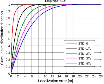
Figure 4 illustrates the increasing of localization error with the increasing of TOA error given by the standard deviation of a Gaussian distribution expressed in multiple of Ts. The figure has form of an empirical Cumulative Distribution Function (CDF). Here, CDF is defined by CDF E( )P E( e) where P E( e) is a probability that the localization error E is less than or equal to e. The CDF in Figure 4 were calculated for the antenna distanced0.5m, the range resolution
0.0333
Sr m and the standard deviationsSTD{0,1 , 2 ,3 , 4 }Ts Ts Ts Ts . The case 0
STD means that TOA was estimated, except for the quantization error, accurately. Then, the localization errors observable in Figure 4 for the red curve line results only from limited number of rays formed from estimated locations.
The maximal error around 6 m appertains to the positions located near the x-axis what corresponds with Figure 2(a). From the red CDF from Figure 4 can be also seen that 90% of all estimated locations has localization error less than 2 m. The increasing of the standard deviation leads to increasing of the maximal
localization error gradually up to 26 m. The localization error for 90% of all estimated locations rises with every consequent value of STD approximately about 2 m (Figure 4).
0 2 4 6 8 10 12 14 16 18 20 22 24 26
0 0.1 0.2 0.3 0.4 0.5 0.6 0.7 0.8 0.9 1
Localization error [m]
Cumulative distribution function
Empirical CDF
STD=0 STD=1Ts STD=2Ts STD=3Ts STD=4Ts
Figure 4
Illustration of the localization error increasing with the increasing of TOA error given by the standard deviation of a Gaussian distribution expressed in multiples of the sample period Ts by
means of the cumulative distribution function
2.3 Maps of Average Localization Errors
Distribution of the localization errors in a monitored area can be demonstrated through the maps of average localization errors. The map is created in the following steps:
the monitored area is divided to subregions,
from every subregion is randomly generated K positions,
for them is calculated exact TOA as round trip time between Tx-the kth position-Rxi for k=1,2,…,K and i=1,2,
every exact TOA is rounded (quantization error) and increased about the expected STD of a Gaussian distribution expressed in multiples of Ts (measuring and processing error),
from the couples of such TOA are computed the position estimates,
the difference between the true and estimated position express the localization error,
for every subregion is computed the average localization error,
finally, all the subregions are depicted in a common map where according to color is possible to distinguish regions with different localization errors.
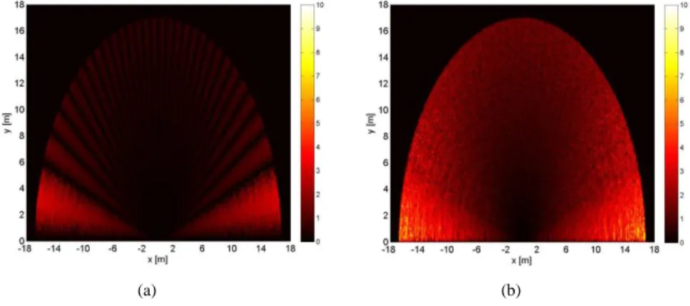
The illustration of three various visual display of the localization error distribution is given in Figure 5 and Figure 6. The first figure depicts accumulation of the localization errors under the same scale of colours expressing the average error from interval 0,10 m. The maps from Figure 5(a) to Figure 5(f) demonstrate the extension of the localization error due to increasing of TOA error. The results complement the information provided by the CDF from Figure 4.
Figure 6 represents a decrease of the localization error depending on the increasing of the distance between antennas. The colour scale adapts to maximal attained localization error. The maps from the first column are depicted also in the form of contour maps in the second column of Figure 6. The contour maps provide a clear understanding of the mutual relation between a given deployment of radar antennas and the achievable accuracy at various target locations. From Figure 6 can be observed the changing shape of the most precise areas.
(a) (b)
(c) (d)
(e) (f)
Figure 5
The maps of average localization errors obtained for d=0.5 m, Sr=0.0333 m and changing TOA error expressed as STD of a Gaussian distribution expressed in multiples of Ts (a) STD=0, (b) STD=1Ts, (c)
STD=2Ts, (d) STD=3Ts, (e) STD=4Ts, (f) STD=5Ts.
(a) (b)
(c) (d)
(e) (f)
Figure 6
The maps of average localization errors obtained for Sr=0.0115 m, STD=3Ts and changing d (a) d=0.1 m, (b) the contour map for d=0.1m, (c) d=0.5 m, (d) the contour map for d=0.5 m, (e) d=1 m, (f) the
contour map for d=1 m
3 Experimental Results
The validation of presented simulation results concerning the localization accuracy of UWB radar operating in complex environment is demonstrated by processing of the signals acquired by two M-sequence UWB radars with different range resolution and coverage [4], [16]. The first UWB radar system, depicted in Figure 7(a), has the range resolution 0.0115 m and coverage of 47 m. The remaining basic parameters are 13 GHz chip clock rate and 4095 impulse response samples regularly spread over 315 ns. During measurement, the radar was equipped with one transmitting and two receiving opened horn antennas (Figure 7(a)).
The second M-sequence UWB radar, depicted in Figure 7(b), has the range resolution 0.0333 m and coverage of 17 m. The remaining basic parameters are 4.5 GHz chip clock rate and 511 impulse response samples regularly spread over 114 ns. During measurement, the radar was equipped with one transmitting and two receiving closed horn antennas (Figure 7(b)).
(a) (b)
Figure 7
M-sequence UWB radars with: (a) the range resolution 0.0115 m and coverage of 47 m, (b) the range resolution 0.0333 m and coverage of 17 m
3.1 Measurement I
The first measurement was realized without an obstacle in the line of sight. The M-sequence radar with the coverage of 47 meters was located together with antennas in the long corridor. The distance between antennas was set to 0.42 m, because the area was narrow, with Tx between Rx1 and Rx2. The measurement scenario was simple – a person was walking from the position in front of Tx 40 m straight and then back with short stopping every 5 m.
The localization results obtained by the signal processing procedure for the detection, localization and tracking of moving targets, described in [13], are depicted in Figure 8(a). Here can be observed that despite of the scenario simplicity the localization errors reach the values above the 20 m. However, such results are consistent with the expected distribution of average localization errors represented in Figure 8(b).
The localization error map was computed for the parameters Sr=0.0115 m, d=0.42 m and STD=9Ts=0.69 ns. The value of STD was found for the used M-sequence UWB radar experimentally on the basis of various measurements. According the environment complexity, average TOA errors recomputed to ranges reach the values between 0.2 m to 0.3 m for human targets. It corresponds with
9 ,13s s
STD T T for Ts 0.0769ns. As the considered measurement was realized without an obstacle in the line of sight, STD=9Ts.
(a) (b) Figure 8
Measurement I: (a) estimated target positions, (b) expected localization errors for the parameters Sr=0.0115 m, d=0.42 m, STD=9Ts=0.69 ns
3.2 Measurement II
The second measurement was more challenging. The M-sequence UWB radar with the coverage of 17 m was located behind 0.17 m thick concrete wall (Fig. 9).
The distance between adjacent antennas was set to 0.38 m (maximal distance enabled by the used tripod), 0.14 m from the wall (Figure 9(a)). The monitored area was short corridor with a staircase depicted in Figure 9(b). During measurement, a person was walking along the corridor up the stairs and then back through the reference positions P1-P2-P1 marked in Figure 9(c).
The localization results obtained by the same signal processing procedure as in the first measurement are depicted in Figure 9(d). As the relative permittivity of the wall was not known, the wall effect compensation phase was omitted. As result, the bias error shifted all the estimated positions further from the radar antennas
(a) (b)
Rx1 Rx2 Tx
P1 P2
0.14m
0.73m 1.47m 0.73m
3.07m 1.8m
0.38m 6.65m
0.17m
(c)
(d) (e)
Figure 9
Measurement II: (a) the antenna deployment behind the wall, (b) interior of monitored area, (c) scheme of the measurement scenario, (d) estimated target positions, (e) expected localization errors
for the parameters Sr=0.0333 m, d=0.38 m, STD=5Ts=1.11 ns
(Figure 9(d)). In addition, the movement near by the rear wall caused the multiple reflections visible in Figure 9(d) for y-coordinate above 2 m.
The best localization accuracy of the target trajectory was achieved in the area 1 m to the left and to the right from Tx. The further parts of target trajectory was estimated with the error higher than 1 m, whereas when the person was walking up and down the stairs the localization error exceeded 2 m (Figure 9(d)).
These results correspond with the expected distribution of average localization errors represented in Figure 9(e). The localization error map was computed for the parameters Sr=0.0333 m, d=0.38 m and STD=5Ts=1.11 ns. Analogous to the
previous case, for the used M-sequence UWB radar holds that for human targets the average TOA errors recomputed to the ranges reach the values between 0.2 m to 0.3 m depending up the environment complexity. It corresponds with
3 ,5s s
STD T T for Ts0.222ns. As the considered measurement was realized through concrete wall with unknown parameters, the standard deviation of the TOA error was chosen 5Ts.
Finally, the tracking results from both considered scenarios are depicted in Figure 10. It can be seen from there that the correctly adjusted tracking system can considerably decrease the localization error.
(a) (b)
Figure 10
The target track estimated for scenario from: (a) measurement I, (b) measurement II
Conclusions
The simulation and experimental results presented in this paper provide practical view on the localization accuracy of UWB radars with minimal antenna array. The obtained maps of the localization errors enable to plan the emplacement of the antenna system depending on the monitored area in advance. They also help to decided about the suitability of the chosen UWB radar for some considered application. The introduced investigation of the localization accuracy taking into account the complexity of the monitored environment can serve as the basis for the analysis of localization accuracy for a sensor network consisted from independent UWB radar systems.
Acknowledgement
This work was supported by the VEGA grant agency under contract No.
1/0563/13 and by the Slovak Cultural and Educational Grant Agency under contract No. 010TUKE-4/2012.
References
[1] Aftanas M., Rovňáková J., Rišková M., Kocur D., Drutarovský M.: An Analysis of 2D Target Positioning Accuracy for M-sequence UWB Radar System under Ideal Conditions, The 17th International Conference Radioelektronika, Brno, Czech Republic, pp. 189-194, April 2007
[2] Blackman S. S., Popoli R. Design and Analysis of Modern Tracking Systems, Artech House Publishers, 1993
[3] Curry G. R.: Radar System Performance Modeling, second edition, Artech House, 2005
[4] Daniels D. J.: Ground Penetrating Radar, 2nd ed. London, UK: The Institution of Electrical Engineers; 2004, chapter M-sequence radar written by Sachs J.
[5] Geogiadis A., Rogier H., Roselli L., Arcioni P.: Microwave and Milimeter Wave Circuits and Systems – Emerging Design, Technologies and Applications, John Wiley & Sons, Ltd., Chichester, November 2012 [6] Gezici S., Tian Z., Giannakis G. B., Kobayashi H., Molisch A. F., Poor H.
V., Sahinoglu Z.: Localization via Ultra-Wideband Radios: A Look at Positioning Aspects for Future Sensor Networks, IEEE Signal Processing Magazine, Vol. 22, No. 4, pp. 70-84, July 2005
[7] Godrich H., Haimovich A. M., Blum R. S.: Target Localization Accuracy Gain in MIMO Radar-based Systems, IEEE Transactions on Information Theory, Vol. 56, No. 6, pp. 2783-2803, June 2010
[8] Jia T., Buehrer R. M.: A New Cramer-Rao Lower Bound for TOA-based Localization, IEEE Military Communications Conference (MILCOM), San Diego, CA, pp. 1-5, November 2008
[9] Kaune R., Horst J., Koch W.: Accuracy Analysis for TDOA Localization in Sensor Networks, Proc. of the 14th International Conference on Information Fusion (FUSION), Chicago, IL, pp. 1-8, July 2011
[10] Kocur D., Rovňáková J., Urdzík D.: Short-Range UWB Radar Application:
Problem of Mutual Shadowing between Targets, Elektrorevue, ISSN 1213- 1539, Vol. 2, No. 4, pp. 37-43, December 2011
[11] Leung S. W., Minett J. W., Chung C. F.: An Analysis of the Shadow Feature Technique in Radar Detection, IEEE Trans. Aero. Elec. Sys., Vol.
35, No. 3, 1999, pp. 1104-1106
[12] Niemeyer F., Born A., Bill R.: Analysing the Precision of Resource Aware Localisation Algorithms for Wireless Sensor Networks, Accuracy Symposium, pp. 41-44, July 2010, Leicester, UK
[13] Rovňáková J.: Complete Signal Processing for through Wall Tracking of Moving Targets, LAP LAMBERT Academic Publishing, Germany, September 2010
[14] Rovňáková J., Kocur D.: Compensation of Wall Effect for Through Wall Tracking of Moving Targets, Radioengineering journal: Special Issue on Workshop of the COST Action IC0803, Vol. 18, No. 2, pp. 189-195, June 2009
[15] Rovňáková J., Kocur D.: TOA Estimation and Data Association for Through Wall Tracking of Moving Targets, EURASIP Journal on Wireless Communications and Networking, The special issue: Radar and Sonar Sensor Networks, Volume 2010, pp. 1-11, September 2010
[16] Sachs J.: Handbook of Ultra-Wideband Short-Range Sensing, Wiley-VCH, December 2012
[17] Tüchler M., Schwarz V., Huber A.: Accuracy of an UWB Localization System Based on a CMOS chip, Proc. of the 2nd Workshop on Positioning, Navigation and Communication (WPNC) & 1st Ultra-Wideband Expert Talk (UET), pp. 211-220, 2005
[18] Yelf, R: Where is True Time Zero?, Proc. of the 10th International Conference on Ground Penetrating Radar, Vol. 1, pp. 279-282, June 2004 [19] Zhang C., Kuhn M., Merkl B., Fathy A. E., Mahfouz M.: Accuracy
Enhancement of UWB Indoor Localization System via Arrangement of Base Stations, Proc. GA, 2008