Iterative parameter identification method of a vehicle odometry model
M´at´e Fazekas,Bal´azs N´emeth, P´eter G´asp´ar
Institute for Computer Science and Control, Hungarian Academy of Sciences, Kende u. 13-17, H-1111 Budapest, Hungary. E-mail:
[mate.fazekas;balazs.nemeth;peter.gaspar]@sztaki.mta.hu
Abstract:The paper proposes an off-line iterative estimation algorithm for wheel circumference estimation of autonomous vehicles. The motivation of the paper is that the signals of the GPS are not available in parking garages or in several urban areas, e.g. next to the buildings with high walls. Therefore, in these situations the wheel encoder based odometry can be an appropriate choice for autonomous vehicle localization, which requires the precise estimation of the wheel circumference. The proposed novel method has three layers, in which the Kalman-filtering with an enhanced tuning method and the least squares algorithm are performed in an iterative loop.
Since the off-line methods uses all of the measurements at once, a highly accurate estimation with low sensitivity on the noise can be reached. The efficiency of the algorithm is presented through CarMaker simulations.
Keywords:parameter identification, autonomous vehicle, vehicle odometry, Kalman-filtering 1. INTRODUCTION AND MOTIVATION
Vehicle localization became a widely research topic in the automotive industry with appearing of the driver assis- tance systems and the autonomous vehicle functions. In the recent years several methods for localization using a wide range of sensors were presented, such as camera, LiDAR, GPS, IMU and wheel encoders. The perception based methods require prior teaching or well recognizable features, see Bloesch et al. (2015). The fusion of GPS and IMU measurements could be precise on higher velocity scenarios, but it assumes the actual knowledge of the covariances of the signals. Moreover, the signals of the GPS are not available in parking garages or in several urban areas, e.g. next to the buildings with high walls. Therefore, in these situations the wheel encoder based odometry can be an appropriate choice for vehicle localization and navigation. However, these localization methods require the model of the vehicle, which can contain parameter uncertainties. Thus, the estimation of some vehicle param- eters is an important feature of the autonomous vehicle localization.
The odometry based on the vehicle model was widely used in mobile robot applications in the last few years, see e.g. Larsen et al. (1999). With the appearing of the the parking assist functions the dead-reckoning localisation be- came standard in the automotive industry (Brunker et al.
(2017a)). The wheel encoder based models are also used in the automated navigation as part of the fusion algorithm
? This work has been supported by the GINOP-2.3.2-15-2016-00002 grant of the Ministry of National Economy of Hungary and by the European Commission through the H2020 project EPIC under grant No. 739592. The work of Bal´azs N´emeth was partially supported by the J´anos Bolyai Research Scholarship of the Hungarian Academy of Sciences and the ´UNKP-18-4 New National Excellence Program of the Ministry of Human Capacities.
see Thrun et al. (2006), where the wheel motion clearly im- proves the result of the localization, when the GPS signals are unavailable. In the odometry based navigation systems the well-calibrated vehicle model is required to ensure the highly accurate pose estimation. A detailed calibration algorithm can be found in Lee and Chung (2008). However, it uses pre-defined paths and assumes precise start and final position measurements. An automated calibration is presented in Larsen et al. (1998), where the reference mea- surements are specific guide marks. Nowdays, in an intel- ligent autonomous system the self-calibration is required, with which the functionallity in varying circumstances i.e. tyre wearing or wheel changing can be guaranteed.
Thus, auto-calibration is requested for wide range of the onboard sensors in an automated vehicle. However, the perception sensor based algorithms often require high com- putation capacity. The IMU measurements are generally inaccurate, because of sensor biases and noises. The GPS measurements are suitable to estimate the real value of the parameters. A self-adaptive method is presented in Brunker et al. (2017b), which deals with the estimation of the time delay of the sensor.
The parameter identification problem is handled conven- tionally with the least squares approximation, while the optimal state estimation at various environmental condi- tions is guaranteed by Kalman-filters, see Crassidis and Junkins (2012). However, the identication of the system parameters of a dynamic model from noisy inputs and outputs is a complex problem. Using a Kalman-filter for the estimation is a potential solution, as presented in Larsen et al. (1998); Freeman et al. (1986); Brunker et al.
(2017b). This application is called in several literature as Augmented Kalman-filter. It handles the system parame- ters as state variables and it modify their values in every iteration step. Thus, a constant value is not achievable and
the effect of the actual noise is higher than the previous noises.
In nonlinear scenarios a possible solution can be the Extended Kalman-filter, which generally operates with a first order Taylor linearization. This calculation is an approximation of the optimal result, in which the normal distribution of the Gaussian variables during linearization is considered. Thus, the estimated states can be biased, see e.g. Freeman et al. (1986); Herzog (2013).
The scope of this paper is to propose a novel iterative parameter identification method for wheel encoder based odometry. The identification algorithm has three main layers, in which a Kalman-filter is designed for state estimation and the result of the fusion is used in a least squares (LS) estimation to determine the values of the parameters. The off-line algorithm estimates the circumference of the wheels, which is a crucial parameter in the model of the on-line odometry. Since the variation of the wheel circumference has a low dynamics, the off-line estimation can be an appropriate solution. The advantage of the method is that it is not necessary to find a balance between the computation time and the preciseness of the estimation due to the off-line computation. In the method an iterative procedure is proposed to improve the preciseness of the parameter identification.
The proposed method can have several other application areas in the autonomous vehicle control, such as the estimation of the vehicle position at low velocities or the determination of the IMU signal bias and covariance values. A well-parameterized vehicle model odometry is often needed for the perception based methods, see e.g.
Funk et al. (2017).
The paper is organized as follows. In Section 2 the two- wheel model of the odometry is presented. Moreover, the iterative parameter identification method is found in Section 3, while the tuning of the estimator is proposed in Section 4. Simulation results are presented in Section 5 and finally, the contributions of the paper and the future challenges are summarized in Section 6.
Motivation examples of the wheel radius identification In the following example the impact of the wheel radius on the vehicle motion is illustrated. The aim of the simulation is to show that the unknown tyre wear can have a high impact on the autonomous vehicle maneuvering, if pure odometry navigation is implemented. Using the high- fidelity vehicle simulation software CarMaker the accuracy of the pose estimation is investigated on account of the uncertainty of the wheel radius on the rear wheels.
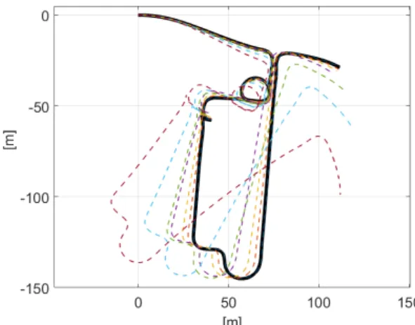
In the examples the nominal tyre radius is 312.6mmand the sampling time is selected as 50Hz. A complex parking- garage maneuvering is analyzed. The tyre wear values on the rear wheels are found in Figure 1, where RL and RR means rear left and rear right. However, the radius values of the wheels are considered to be the nominal value in the odometry of the navigation system. The resulted errors can be found in Table 1 as well. The estimated paths with various tyre wear values are presented in Figure 2.
Fig. 1. Pose errors in a parking garage scenario
Fig. 2. Position data with different tyre wear
The results show that small deviation from the nominal wheel radius can lead to a significantly different course of the vehicle. However, another conclusion of the motivation example is that the precise estimation of the actual wheel radius can result in an appropriate vehicle motion. Thus, if the wheel radius can be estimated precisely, it can be used for long distance navigation in the areas without GPS, or in the areas with imprecise GPS signals.
2. TWO-WHEEL VEHICLE MODEL OF THE ODOMETRY
The dead-reckoning navigation is based on a model, of which state vector xkcontains the longitudinal and lateral vehicle positions xk, yk and the heading angle θk. The inputs of the system are the longitudinal vk and angular ωk velocities of the reference point, which can be the midpoint of the rear track. The only difference between the odometry models is the calculation of these velocities. The wheel encoder based odometry models use the rotation encoders of all wheels and the wheel angle encoders of the front wheels. In case of a two-wheel model based odometry the angular velocity is calculated only from the front wheel angles. However, in this paper the main focus is on the parameter identification, therefore the estimation method is based on the two-wheel odometry model, in which both velocities contain the wheel radius parameter.
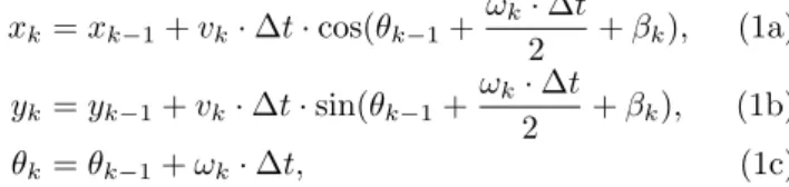
The planar motion of the vehicle is calculated as
xk=xk−1+vk·∆t·cos(θk−1+ωk·∆t
2 +βk), (1a) yk=yk−1+vk·∆t·sin(θk−1+ωk·∆t
2 +βk), (1b)
θk=θk−1+ωk·∆t, (1c)
where βk is the side-slip angle of the vehicles. However, during the identificationβk≈0 is assumed.
The velocities are calculated through the rear wheel speeds, which are resulted by the wheel rotation measure- ment and the wheel circumference, such as
vk =nRL,k·cRL+nRR,k·cRR
2·∆t , (2a)
ωk =nRR,k·cRR−nRL,k·cRL
tR·∆t , (2b)
whereni is the rotation number of the wheel,ci = 2πriis the wheel circumference, ri is the dynamic wheel radius, tRis the rear track and ∆tis the sampling time.
3. ITERATIVE METHOD OF THE OFF-LINE PARAMETER IDENTIFICATION
The accuracy of the presented odometry model highly depends on the calibration of the kinematic parameters.
For example, the variation in the track width is less significant, while the deviation from the nominal wheel circumference is more significant due to the vertical wheel load and the tyre wear. Thus, the accuracy of the model based estimation highly depends on the real value of ci. The identification uses the onboard sensors, such as the measurement of GPS position, the magnetic heading, the MEMS acceleration, the yaw-rate from the gyroscope and the wheel rotation. The process of the iterative solution is illustrated in Figure 3.
Fig. 3. Process of the iterative parameter estimation The method has three main layers, in which the Kalman- filtering and the Least Squares optimization are connected
together in an iterative way. This approach can also be feasible for identification of Hammerstein and Wiener models, see in Ma et al. (2017).
3.1 Calculation of the reference signal
The GPS and IMU measurements are fusioned to reach the absolute position and orientation valuesexk= [xek,eyk,θek]T, which are considered as references for the computation.
This fusion method has been investigated already in a wide range of papers considering the dynamic equation of ¨p=a, wherepis the position andais the acceleration.
The implemented method is similar to Caron et al. (2006).
In the fusion of this layer the measurement of the wheel encoders are not used.
3.2 Design of the Kalman-filter
The inputs of the two-wheel vehicle model are measured with the wheel encoders
uk−1= [nRL,k−1·cRL nRR,k−1·cRR], (3) whereni,k−1 represents the rotation number of the wheel from the encoders. The resulted nonlinear system model is
xk=f(xk−1,uk−1), (4) which contains the equations of the two-wheel model (1).
The core of the method is the design of an Extended Kalman-filter, which uses the wheel encoders as inputs, the reference position and the orientation values, which are generated through the first layer as measurements.
Moreover, the nonlinearity is approximated with the first derivative of the system model. The filtering of ˆxk = [xk, yk, θk]T is performed in the following two steps.
• Prediction based on the model The predicted states and covariance matrix are calculated as follows
ˆ
x−k =f(ˆxk−1,uk−1), (5a) Σ−k =FkΣk−1FkT +P, (5b) where the Jacobian is stated as follows and compute in the previous state as
Fk = ∂f(x,u)
∂x x=ˆx
k−1,u=uk−1
. (6)
• Innovation based on the measurements In the innovation phase the measurements are used to im- prove the estimation. The state and the covariance calculated as follows
ˆ
xk = ˆx−k +Gk(yk−h(ˆx−k)), (7a) Σk = (I−GkHk)Σ−k, (7b) where h(x) is the measurement equation, which is h(x) = [xk, yk, θk]T. The Jacobian is stated asHk = I and the measurement vector is yk = xek. Gk is the Kalman-Gain factor, which ensures the optimal estimation of the states and guarantees the minimum covariance. The gain equation follows as
Gk = Σ−kHkT(HkΣ−kHkT +M)−1. (8) The estimation highly depends on theP andM matrices, which are the model and measurements covariances. The tuning and the setting of the proper values of these matrices are found below in Section 4.
3.3 Least squares method in the iterative design
The LS approximation is the conventional method for parameter identification, when algebraic equations can be formed between the measured and the estimated parame- ters. The relationship is generally formulated as
zk
|{z}
Z
= φk
|{z}
Φ
ϑ+εk, (9)
where zk is the measurement, φk contains algebraic func- tions and other measurements,εsymbolizes the measure- ments noise andϑis the parameter vector to be identified.
The resulted solution of the optimal parameter values are ϑˆ= (ΦTWΦ)−1ΦTW Z (10) where W is a positive definite weighting matrix. The coefficients ofW are set asdiag([1 1 10]) to compensate the effect of 1mlateral or longitudinal and 1radheading errors. In the presented estimation method the algebraic function is formulated using a fusioning method. The fusioned states are resulted by the filter of the second layer and the calculated references of the first layer, such as
exk =f(ˆxk−1,uk−1). (11) The relation is ordered in the form of (9) as follows:
zk =
xek−ˆxk−1 eyk−yˆk−1 θek−θˆk−1
, (12a)
φk =
nRL,k
2 ·cos(ˆθk−1) nRR,k2 ·cos(ˆθk−1)
nRL,k
2 ·sin(ˆθk−1) nRR,k2 ·sin(ˆθk−1)
−nRL,kt
R
nRR,k tR
, (12b) ϑ= [cRL cRR]T. (12c) The second and the third layers of the presented algorithm run in an iterative loop to guarantee the right approxima- tion of the real parameter values.
4. TUNING METHOD OF THE KALMAN-FILTER The Kalman-filter estimation highly depends onP andM covariance matrices, as it has already been stated in the previous sections. Generally, the matrices are considered in diagonal form and the coefficients ofM are the deviations of the sensors. The values of P are calculated from the effect of the deviations of the inputs on the system model.
In the presented method the goal is to improve the identification method of the system parameters to reach a more accurate estimation. Thus, the Kalman-filter of the second layer must guarantee the convergence to the real values during the iterations. In practical applications these values are unknown, and thus a grid search or an a priori fix setting of the matrices are not suitable.
The proposed tuning method operates with the mean deviation from the reference, which is calculated in the first layer of the estimator. After the LS optimization in the iterative loop the two-wheel vehicle model (1) with the new parameters is simulated on the whole dataset. Then, the mean position and orientation errors from the results are calculated. The iterative estimation persists until the errors are not increased permanently. The convergence towards the real parameter values is guaranteed through the appropriate selection of P and M matrices. The
experiences show that the ratio of the coefficients has more impact on the result of the estimation, related to the specific numerical values.
The measurement covariance values are selected to be constant, while the model covariance matrix is varied in every iteration steps as follows. In the early steps, when the model uncertainty is high, due to the inaccurate wheel parameters, the coefficients are higher than the values of matrixM. Step by step assuming the continuous learning of the real parameters, the values of the M matrix are steadily decreasing. Thus, the covariance matrices are set to
M =diag([1 1 0.01]), (13a) P =diag
150 iq
150 iq
15 iq
, (13b)
wherei is the actual iteration number andqis a variable in the range of 1≤q≤2.
5. SIMULATION RESULTS
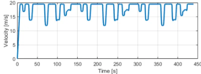
The efficiency of the proposed estimation method is demonstrated through various simulation examples, using the high-fidelity vehicle dynamic software CarMaker. It is assumed that the measured signals contain noises, which have Gaussian distribution and the standard deviations of the sensors are σGP S = 3, σAcc = 0.2, σY awR = 0.02, σHead = 0.15. The measurements are generated with a sedan passenger car, which is driven along 3 laps of the Hockenheim race track. The velocity profile and the path of the track are found in Figure 4 and in Figure 5, respec- tively.
Fig. 4. Velocity profile
Figure 7 presents the results of the wheel circumference estimation using the proposed iterative off-line method.
The mentioned auto-tuning scheme guarantees the con- vergence. When the local minimum has been reached, the iteration has been stopped, see Figure 6, where the red dashed line shows the stop of the iteration step. The rest of the iterations are only done for illustration proposes.
The errors of the parameters are ∆cRL = 0.41 mm and
∆cRR= 0.43mm, whose relative error is lower than 0.05
%. The mean error from the ground reference is 7.87 m and 0.93◦, the maximum errors are only 15m and 4.58◦. These are small values in the field of recursive odometry methods, since the overall traveled distance is more than 7.5 km.
Moreover, for the analysis of the proposed method the simulation is performed 10 times on the track with re- generated noises. The result of the circumference estima- tion is presented in Figure 8. The mean of the absolute
Fig. 5. Path of the reference track
Fig. 6. Errors of iterations
Fig. 7. Iterations of wheel circumference estimation deviation from the real value of the circumference is 0.86 mm and the maximum error is less than 1.5 %. The efficiency of the auto-tuning scheme is also demonstrated in Figure 8. The simulations are performed, when the P matrix of the Kalman-filter is settled to an appropriate constant value (Fix RL-RR). The results show that the mean of the absolute error is 1.6 times higher (1.39mm) than the error of the iterative solution with various model covariance. Thus, the iterative solution with the proposed tuning method has high efficiency.
Figure 8 shows that in the second and third scenarios the solution with the varying covariance results in a less precise circumference estimation. However, the mean errors in the position and the orientation are smaller, see Figure 9 and Figure 10. Thus, these results confirm that the iteration must be stopped at the minimum value of the mean position and orientation error - even if the circumference
Fig. 8. Result of the simulation scenarios
error is slightly increased, see Section 4. It can be avoided with the consideration of βk, but can result in a more complex estimation method.
Fig. 9. Position error the simulation scenarios
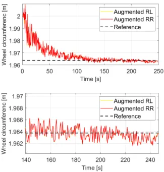
Fig. 10. Orientation error of the simulation scenarios For comparison purposes, the estimation is also performed using the mentioned Augmented Kalman-filter in the in- troduction section. The estimatedcRL, cRRare acceptable in both of the methods, see Figure 11. The mean of the absolute deviation from the real circumference is reduced around 50% and the variance is significantly smaller with the iterative method. The explanation of this result is that the off-line iteration uses all of the measured signals at once, which results in a smaller sensitivity of the results on the noises. In contrast the augmented method estimate the parameters in every timestamp. Furthermore, the dynamic wheel radius can change in the corners due to the lateral dynamics. This and the effect of the actual noise probably result noisy estimation of the wheel circumference param- eters. Figure 12 shows the value of the parameters at the augmented method in a concrete scenario. The converga- tion to the true value is appropriate, however the changing of the value between the timestamps is significant, the process can identify the wheel circumference only with
Fig. 11. Comparison of the estimation method
a 2 mm uncertainty. Therefore the determination of a constant final value is not evident.
Fig. 12. Augmented Kalman-filter method 6. CONCLUSIONS
The paper proposed an off-line iterative estimation algo- rithm for a wheel circumference estimation, which has high accuracy. The method has three layers. First, a reference signal calculated, which is fusioned with a two wheel odometry model in a Kalman-filter algorithm in the second layer. Thirdly, a parameter identification based on a least squares method is performed. The estimation runs in an iterative loop, where the convergence to the real values is guaranteed by a tuning method with various covariance matrices. Since the off-line methods uses all of the mea- surements at once, a highly accurate estimation with low sensitivity on the noise can be reached. The efficiency of the algorithm is presented through CarMaker simulations.
As a future challenge, the applied vehicle odometry model might be improved through the consideration of the lateral
dynamics. Through the improved model the changing of the tyre radius in corners and the variation of the vertical load can be considered.
REFERENCES
Bloesch, M., Omari, S., Hutter, M., and Siegwart, R.
(2015). Robust visual inertial odometry using a direct EKF-based approach. InIEEE/RSJ International Con- ference on Intelligent Robots and Systems (IROS), 298–
304.
Brunker, A., Wohlgemuth, T., Frey, M., and Gauterin, F.
(2017a). Odometry 2.0: A slip-adaptive UIF-based four- wheel-odometry model for parking. In IEEE Transac- tions on Intelligent Transportation systems.
Brunker, A., Wohlgemuth, T., Michael, and Gauterin, F. (2017b). GNSS-shortages-resistant and self-adaptive rear axle kinematic parameter estimator (SA-RAKPE).
InIEEE Int. Vehicles Symposium, Los Angeles, USA.
Caron, F., Duflos, E., Pomorski, D., and Vanheeghe, P. (2006). GPS/IMU data fusion using multisensor Kalman filtering: Introduction of contextual aspects.
Information Fusion, 7, 221–230.
Crassidis, J.L. and Junkins, J.L. (2012). Optimal Estima- tion of Dynamic Systems. CRC Press.
Freeman, J., Hassan, F., and Morton, D. (1986). Kalman filter parameter identification: a practical approach.
Transactions of the Institute of Measurement and Con- trol, 8(1), 24–28.
Funk, N., Alatur, N., Deuber, R., Gonon, F., Messikom- mer, N., Nubert, J., Patriarca, M., Schaefer, S., Sco- toni, D., Bnger, N., Dube, R., Khanna, R., Pfeiffer, M., Wilhelm, E., and Siegwart, R. (2017). Autonomous electric race car design. InEVS30 Symposium, Stuttgart, Germany.
Herzog, F. (2013). Kalman filter and parameter identifi- cation.
Larsen, T.D., Bak, M., Andersen, N.A., and Ravn, O.
(1998). Location estimation for an autonomously guided vehicle using an augmented Kalman filter to autocali- brate the odometry.
Larsen, T.D., Hansen, K.L., Andersen, N.A., and Ravn, O. (1999). Design of Kalman filters for mobile robots;
evaluation of the kinematic and odometric approach.
InIEEE International Conference on Control Applica- tions.
Lee, K. and Chung, W. (2008). Calibration of kinematic parameters of a car-like mobile robot to improve odom- etry accuracy. In IEEE International Conference on Robotics and Automation.
Ma, J., Ding, F., Xiong, W., and Yang, E. (2017). Com- bined state and parameter estimation for hammerstein systems with time delay using the kalman filtering.
International Journal of Adaptive Control and Signal Processing, 31.
Thrun, S., Montemerlo, M., Dahlkamp, H., Stavens, D., Aron, A., Diebel, J., Fong, P., Gale, J., Halpenny, M., Hoffmann, G., Lau, K., Oakley, C., Palatucci, M., Pratt, V., Stang, P., Strohband, S., Dupont, C., Jendrossek, L., Koelen, C., Markey, C., Rummel, C., van Niekerk, J., Jensen, E., Alessandrini, P., Bradski, G., Davies, B., Ettinger, S., Kaehler, A., Nefian, A., and Mahoney, P.
(2006). Stanley: The robot that won the DARPA Grand Challenge. Journal of Field Robotics, 23(9), 661–692.