Developing Stability Control Theories for Agricultural Transport Systems
Tamás Szakács
Institute of Mechatronics and Autotechnics
Bánki Donát Faculty of Mechanical Engineering and Security Technology Óbuda University
Népszínház u. 8, H-1081 Budapest, Hungary E-mail: szakacs.tamas@bgk.uni-obuda.hu
Abstract: The design and management of agricultural transport systems is facing a series of challenges. The goals of increasing vehicle mobility and reducing soil stress have always been in the center of attention. Involving trailer wheels in the production of pulling force could be beneficial in both cases. In this way, the mobility of the transport system could be secured even in heavy soil conditions, and the soil damage could be reduced as well.
Despite the potential advantages, trailer protrusion is not currently practical. The reason for this is the lack of proper safety measures. The origin of this problem is the force generated by the trailer protrusionacting on the drawbar, which can bring the tractor into an unstable state, causing the tractor to roll over or the vehicle train to jack-knife. To avoid such accidents, a control system must be developed which can recognize the beginning of unstable vehicle behavior and either by warning or intervention help to maintain the stable state of the vehicle.
The goals of this paper can be summarized as follows:
– To introduce a computer simulation model of an agricultural transport vehicle-park consisting of different dynamical models of tractors and trailers. The aim of this model- park is to perform stability analysis of tractor – propelled axle trailer vehicle combinations.
– To introduce stability criteria equations for future stability control programs which can determine different unstable states, and by interaction can re-stabilize the vehicle combinations.
Keywords: Vehicle-train; stability; agricultural transport systems
1 Introduction and Motivation
The subject of this paper is the stability analysis of transport vehicle combinations consisting of agricultural tractors and propelled axle trailers, and the reduction of accidents related to the trailer drive. Special attention has been paid to the accidents caused by the trailer protrusion. In order to achieve the stability increase, I have developed a computer model of a transport vehicle park, which is capable of performing dynamical simulations of transport vehicle trains and which can be the basis for developing stability control theories.
Propelled axle agricultural trailers, and the related problems:
Tractors involved in heavy agricultural transporting tasks are ballasted by extra weights in order to make it possible to produce the pulling force which is required to move the trailer in heavy soil conditions. In my opinion instead of ballasting the tractors, it could be more beneficial to involve the wheels of the trailer in the force development to move the train. This could secure the mobility of the transport system in heavy soil conditions, and the soil damage could be reduced as well.
Involving the wheels of the trailer in the production of the pulling force has the following possible advantages:
- Despite the general tendency towards increasing power in agricultural machinery, the weight of the tractor can be reduced.
- By means of optimized weight and driving torque distribution, soil damage, environmental pollution and operation costs can be reduced.
- By making the transport system more independent from soil conditions, harvesting losses can also be reduced.
Despite the potential advantages, because of the lack of safety measures, trailer protrusion is not part of practical life. The origin of the problem is that the trailer can generate a side force on the rear wheels of the tractor, which under certain conditions can bring the tractor into an unstable state. The trailer can cause the tractor to roll over or to jackknife.
The conclusion can be drawn, that the tractor-trailer vehicle combination can only be used when it is equipped with a control system that can avoid the trailer drive originated accidents to happen.
2 The Models Used for Developing the Stability- Programs
In this chapter the models used for the stability analysis of the agricultural transport vehicle trains and the methods of instability-determinations are briefly introduced. The models I have developed in Matlab/Simulink environment are created for this work. The models are developed in a modular system so that they can be used for the simulation of other types of vehicles in addition to agricultural transport systems. During the development phase, special expectations of agricultural transport systems have been taken into consideration.
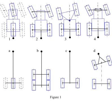
2.1 The Vehicle Model Park Developed for the Task
In order to model agricultural transport systems, I have developed dynamic models of different tractors and trailers. From the model, vehicle combinations can be created as in the reality.
1 2 3 4
a b c d
Figure 1 Vehicle model park
Figure 1 shows the modelled agricultural transport vehicle park. Available tractors are a single-track tractor (1), a system-tractor (2), a joint-tractor (3), and a common ploughing tractor (4). The trailers available are a single-track trailer (1), a semi-suspended tandem axle trailer (2), a semi-suspended single axle trailer (3), and a pulled trailer (4).
The models are created in a Matlab/Simulink environment and built in a modular system. This ensures that different sub-models can be changed within models, and new model units (like a trailer behind a car, a plough behind an agricultural tractor, or a different tractor) can be inserted in the vehicle model if the simulation goals require it.
I have created an animation-window, which helps via simplified schemas of the vehicles to follow the motion of the vehicle train. It has indications for the state of the stability control system, and helps to create animations for demonstration goals.
2.2 Determination of the Pulling Angle
Pulling angle: (Also tow angle (ProPride Inc.)) The horizontal component of the angle between the pulling and the pulled vehicle. Notation: γ (o or rad)
δL
δR
B w γ
γ γ2 γ1
ltr
wC
lpót
lk
rB rlk
A w
rC
sptr sppót
Figure 2
The extended Ackermann-condition of vehicle trains
One method of determining the state of the vehicle is based on measuring the pulling angle and comparing its value to the expected one. To determine the expected value of the pulling angle, I have introduced the extended Ackermann conditions of steered wheel angles to vehicle trains. Figure 2 shows a tractor and a
trailer attached to it. The angles of the steered wheels (δL, δR) are calculated in the conventional manner of Ackermann’s method (Ackermann, 1990).
The Ackermann condition of vehicle train is fulfilled when not only the axles of the wheels of the tractor but also the wheels of the trailers are pointing in the theoretical turning center (momentan centrum). The γstat pull-angle in the steady curving can then be calculated using the notations of Figure 2 as follows:
γstat=γ1+γ2 (1)
where
⎟⎟⎠
⎜⎜ ⎞
⎝
= ⎛
B k
r arctan l
γ1 and (2)
⎟⎟
⎠
⎞
⎜⎜
⎝
⎛
= +
⎟⎟⎠
⎜⎜ ⎞
⎝
= ⎛
) arcsin (
arcsin
γ2 2 2
B k
pót lk
pót
r l
l r
l . (3)
Equations (2) and (3) substituted in eq. (1):
⎟⎟
⎠
⎞
⎜⎜
⎝
⎛ + +
⎟⎟⎠
⎜⎜ ⎞
⎝
= ⎛
) arcsin (
arctan
γ 2 2
B k
pót B
k
stat l r
l r
l (4)
The turning radius of the rear axle is:
2 w ) tan(δ
r l A
L tr
B= + (5)
The calculated steady state γstat pulling angle is equivalent only in steady curving with the actual pulling angle. The reason for this is that in contrast to the δL, δR
steering angles of front wheel of the tractors, which immediately occur as the steering wheel is turned, the pulling angle is continuously changing as the vehicle moves. To reach its steady state value, the vehicle has to travel a certain distance.
My goal was to set up a model or equation which describes the actual value of the pulling angle, not only in steady but also in transient state.
A -
γ
stat+ ∫ γdyn
Figure 3
Determination of γdyn actual pull-angle based on the γstat steady-state pull-angle
Figure 3 shows the block scheme realization of the transient state pull-angle determination. In this case, the matrix A is simplified to scalar, and its value is the reciprocal of the time required by the rear axle of the trailer to reach the position of the rear axle of the tractor.
In equation:
k pót
tr x
l l A v
= + , (6)
where vtrx is the speed of the tractor (in m/s), lpót+lk is the distance of the axles of the tractor and the trailer (in meters).
The actual value of the pulling angle in a differential equation form:
stat din
din γ γ
dt dγ A
1 + = (7)
The solution of the equation depends on the input function (γstat). Using a step input function with the amplitude of γstat, the equation of γdin output will be:
(
-At)
stat
din γ 1 e
γ = − . (9)
2.3 Stability Determination
The stability determining functions are logical criteria functions of which the value is 0 if the vehicle behaves as expected, and 1 if instability is detected.
The general form of the criteria equations is:
[ ]
[ ]
⎩⎨
⎧
∉
∧
>
∈
∨
= <
high low
high low
ected ected
measured ected
ected if
ected ected
measured ected
ected stab if
exp exp
exp exp
, 1
exp exp
exp exp
, 0
min min
…
… (10)
where:
- expected is the calculated value of the stability determining parameter.
- expectedmin is the threshold value of the expected parameter. If measured lower is expected, then no stability validation is done,
- expectedlow is the lower limit of the reference band used in the comparison of expected and measured values,
- expectedhigh is the upper limit of the reference band used in the comparison of expected and measured values.
The expected values and the stability determining method can then be embedded in vehicle and Fuzzy logic controller design, and its application as an embedded system can be considered as well. (Farkas, Halász, 2006)
3 Validations by Field Measuring
Figure 4
Schematic drawing of the measured tractor-trailer combination (Horváth, 1996)
3.1 Combined Braking and Steering Test
Figure 5
Measuring stages of the combined braking and steering test
I have done the validations using a vehicle combination consisting of a Hungarian made SR-10 type propelled axle forwarder attached to a Landini Landpower agricultural tractor.
The measurements were performed on the lands of the forest of Kisalföldi Erdőgazdaság Rt. at the Ravazdi Erdészet location. The measuring track is shown in the Figure 5. The steady-state stage is 30 metres long, and the braking stage is also 30 meters. The steering angles are from a to d 0, 7, 15, and 28 degrees (measured on the front left wheel).
The measurements were performed on a dry sunny day, with temperatures in the range of 20-23oC. The soil was a brown forest soil, permanently maintained, grass covered clearing.
During the taking of the measurement, data were partially manually and partially electronically recorded. The measuring sets became a code for further pairing of the corresponding manually and instrumentally recorded data.
The vehicle-train, after a pre-stage travels, at the second stage either proceeded straight ahead or took a turn with the steering wheel turned to 7, 15 or 18 degrees (a-d variations in the Figure 5), while at the same time decelerating to still-stand by the smooth application of the brakes. The measurement is continued till the still-stand of the vehicle. During the measurement, the steering-wheel angle, the pulling angle, and the acceleration were recorded by a data recording system, and the number of the rotations of the wheels, the time required to pass stages 1 and 2, the speed of the tractor, and a trigger signal were recorded manually. Having completed the first series of measurements, two similar sets of measurements followed. In this way three repetitions were performed.
The goal of the test is to determine the accelerations, wheel slips and curving stability during braking and combined braking and steering.
3.2 Roundabout Test
One of the stability programs is based on measuring the pulling angle between the tractor and the trailer. The roundabout test is to validate the determination of the expected value of the pull angle in steady and transient states. The first stage is a lead up, while the second stage is a roundabout at the maximum steering angle of the tractor. Figure 6 shows the plan of the test and details. In this test only the trailer drive was applied.
Figure 6
Plan and data of the roundabout test
3.3 Validation Test
Figure 7
Plan and data of the validation test
The validation tests were performed in an empty barn, which was under construction. The barn had fine sand and a level bedding, which appeared ideal and easily reproducible. In the bedding I marked a short stage to achieve a near steady-state running of the vehicle combination, followed by either a 20-meter- long straight track, or a left turning one. The same data sets were recorded as in case of the combined braking and steering test. The goal of the measuring was to check the functionality of the measuring instruments, and to perform measurements to validate the pull-angle and yaw-rate determinations.
4 Processing the Measuring Data and Results 4.1 Evaluation of the Braking and Steering Test
0 5 10 15 20 25 30 35 40 45 50
0 5 10 15 20 25
Series1 Series2 Series3 Series4 Poly. (Series3) Poly. (Series4)
Steering angle δ(o)
right left
Wheel slip s(%)
slip_l slip_r av. slip_l av. slip_r
trend. slip_l trend. slip_r
Figure 8
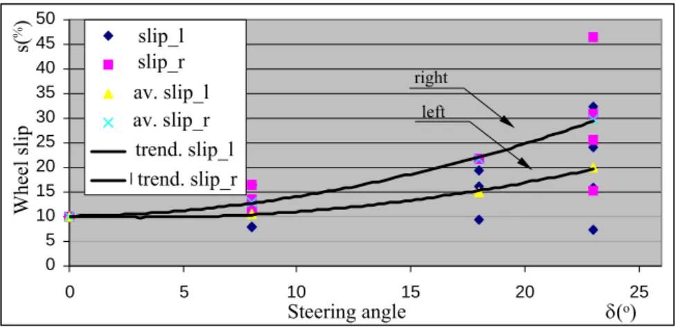
Wheel slips as function of steering angle
Figure 8 shows the dependency of the slip of the driven wheels as a function of the steering angle. The continuous line is a tendency curve drawn over the average calculated slip at the set steering wheel angles. It can be seen that the slip differentiates between inner and outer wheels in the respect of turning direction.
The slip of the inner wheel is proportionally greater than the outer, depending on the steering angle. The averages of the slip values rise proportionally with the steering angle. The reason for this is that the travelling losses increase with the steering angle, and the increased losses indirectly cause increased slip values.
4.2 Evaluation of the Roundabout Test
The goal of the roundabout test is to bring the vehicle train to an extreme state in order to validate the stability program and the calculation method of the pulling angle. During the test only the trailer drive was used with the steering angle set at 28 degrees to the right.
Data recorded during the test were:
- Numbers of rotations of the trailer tires (nb, nj) - Accelerations of the trailers body (aA1x- aA4y) - Steering angle (δ)
- Pulling angle (γ)
- Travel speed of the train (vh)
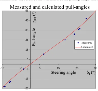
Figure 5 summarizes the result of the validation of the pulling angle calculation.
-25 -15 -5 5 15 25 35 45 55
-15 -5 5 15 25 35
Mért Számított
Measured and calculated pull-angles
Steering angle δl (o) Pull-angle γstat (o )
Measured Calculated
Figure 9
Comparison of measured and simulated pulling angle
Figure 9 shows the comparison of the calculated and the measured steady-state pulling angles. The continuous line shows the function of equation 4, and the squares are the date gained from the field measuring. This result validates the determination of the steady-state pull-angle determination.
From the recorded measurement data, the steering and pull angle data have been taken (Figure 10 upper part). I have created a computer model of the vehicle train and set the parameters in accordance with the measured vehicle. Using the recorded speed and steering data, I have reproduced the simulation with the model. The pull angle produced by the simulation then was compared with the measured one (Figure 10 lower part), after which after I draw the following conclusions. The model used for determining the transient state of the pulling angle gives satisfactory results; therefore, it can be used as the parameter of vehicle stability determination.
Time t(s)
Time history of the steering and the pulling angle
- Steering and pulling angleγ(o)
steering angle
pulling angle
Measured and simulated pulling angles
Pulling angle γ (o)
simulated
measured
Time t(s)
Figure 10
Comparison of measured and simulated pulling angle
Conclusions, summary
Stability determinations were developed using a self-developed model park of agricultural transport vehicles. Among the stability determination methods, the pulling angle based determination proved to be the most accurate, and the easiest to measure its determination parameter. The pulling angle determination model was validated by a series of field measurments. The expected pulling angle can be compared with the measured one, and from the deviation the stability of the vehicle train can be determined. The advantage of this method is that the pull angle deviation can be caused both by the pulling vehicle and the trailer; in this way abnormal behavior of either of them can be determined.
Acknowledgments
The author would like to express his appreciation to the Forestry of of Kisalföldi Erdőgazdaság Rt. for providing the vehicles, area and the crew for the measuring, and prof. Pérer Szendrő and Lajos Laib for the support, as well as the leaders of Óbuda University for providing the working conditions.
References
[1] Towing Definitions on the ProPride Inc. home page.
http://www.propridehitch.com/trailer_sway/towing_definitions.html downloaded at 02.01.2010
[2] Mitschke, M: Dynamic der Kraftfahrzeuge. 2. Auflage, Band C, Berlin Springer 1990
[3] Ferenc Farkas, Sándor Halász: Embedded Fuzzy Controller for Industrial Applications, Acta Polytechnica Hungarica, Vol. 3, No. 2, 2006, pp. 41-63 [4] Horváth Béla (Editor): SR-8 kihordó gépesítési információ Panax Kft.
Nyomdaüzeme, 1996, p:30