Implementation of Medical Imaging Algorithms on Kiloprocessor Architectures

(1)

Implementation of Medical Imaging Algorithms on Kiloprocessor Architectures

G´ abor J´ anos Tornai

Faculty of Information Technology and Bionics P´ azm´ any P´ eter Catholic University

Scientific Advisor:

Gy¨ orgy Cserey Ph.D.

Consulent:

Tam´ as Roska DSc.

A thesis submitted for the degree of Ph.D.

Budapest, 2014

(2)

(3)

I would like to dedicate this thesis to my loving wife, my children and parents ...

Love never fails. But where there are prophecies, they will cease;

where there are tongues, they will be stilled; where there is knowledge, it will pass away. For we know in part and we prophesy

in part, but when completeness comes, what is in part disappears.

When I was a child, I talked like a child, I thought like a child, I reasoned like a child. When I became a man, I put the ways of

childhood behind me. For now we see only a reflection as in a mirror; then we shall see face to face. Now I know in part; then I

shall know fully, even as I am fully known. 1 Cor 13,8-12

(4)

Acknowledgements

I deeply thank Tam´as Roska and P´eter Szolgay the former and the present head of the doctoral school for their advice and encouragement giving me the strength to go on.

It is hard to precisely articulate how I thankGy¨orgy Cserey my advisor the fascinating work lasting more than seven years. Without his excellent ideas and inspiration I would not have been successful in my doctoral studies. We managed to find a way to discuss the real life problems and joys as well.

I thank Ion Pappas his support, encouragement, advices, and inspiration. During our collaboration I learned how industry and academy can benefit from each other.

I thank Barnab´as Garay for guiding my first steps in the world of partial differential equations. Additionally, he showed me how math- ematicians treat problems. Thanks for the great impression.

To the other doctoral students: András Horváth, Attila Stubendek, Domonkos Gergely, Miska Radványi, Tamás Fülöp, Ádám Rák, Tam Zsedrovits, Miki Koller, Csaba Józsa, Csaba Nemes, Bence Borbély, Zoli Tuza, Jani Rudan, Dóri Bihari, Anna Horváth, András and Zsolt Gelencsér. Thanks for the chat near the lunch, the help, the seminars on Fridays, and the other activities.

I thank Vida Tivadarn´e Katinka her eternal service and patience to make the administrative side of life much easier, the work of the dean’s office, the administrative and financial personnel.

I had some really great teachers who should be mentioned here as well. I am grateful to Zsuzsanna Vágó, Miklós Rásonyi, János Lev-

(5)

endovszky and Árpád Csurgay from the Faculty, Mária Bertalan and Katalin Szabó from Reformed Collage Secondary School of Debrecen.

The ¨Oveges scholarship of General Electric Healthcare and the datasets provided by the company are gratefully acknowledged.

The support of grants Nos. T ´AMOP-4.2.1.B-11/2/KMR-2011-0002, and T ´AMOP-4.2.2/B-10/1-2010-0014 are gratefully acknowledged.

Thank you Father, Mother, Piri, Tam´as, Ildi and the whole family.

Everything.

Niki, Magdi and Blanka. You are worth fighting for, and it is a great joy to return back home to you.

(6)

Abstract

This dissertation presents two specific fields of medical imaging: (i) fast digitally reconstructed radiograph (DRR) generation on Graph- ical Processing Units (GPUs) allowing two dimensional to three dimensional (2D to 3D) registration to be performed in real-time and (ii) several sides of the level-set (LS) based methods: theoretical aspects such as initial condition dependence and practical aspects like mapping these algorithms on many core systems.

The generation of DRRs is the most time consuming step in intensity based 2D x-ray to 3D (computed tomography (CT) or 3D rotational x-ray) medical image registration, which has application in several image guided interventions. This work presents optimized DRR rendering on graphical processor units (GPUs) with optimization rules and compares performance achievable on several commercially available devices. The presented results outperform other results from the literature. This shows that automatic 2D to 3D registration, which typically requires a couple of hundred DRR renderings to converge, can be performed on-line, with the speed of 0.5-10 frames per second (fps). Accordingly, a whole new field of applications is opened for image guided interventions, where the registration is continuously performed to match the real-time x-ray.

I investigated the effect of adding more small curves to the initial condition which determines the required number of iterations of an LS evolution. As a result, I discovered two new theorems and devel- oped a proof on the worst case of the required number of iterations.

Furthermore, I found that these kinds of initial conditions fit well to many-core architectures. I have shown this with two case studies, which are presented on different platforms. One runs on a GPU

(7)

and the other is executed on a Cellular Nonlinear Network-Universal Machine (CNN-UM). Additionally, segmentation examples verify the applicability of the proposed method.

(8)

Nomenclature

Roman Symbols

B Diameter of an object D Domain of φ

F Driving force, also known as speedfield of the LS equation F driving force of LS equation

N(.) Neighborhood set of the argument Greek Symbols

φ LS function

Γ Background region

γ interface (curve, surface) to be tracked Ω Object region

τ time constant of the CNN cell Acronyms

AP Anterior-Posterior

API Application Programming Interface ASIC Application Specific Integrated Circuit

(12)

CBCT Cone Beam Computed Tomography CNN Cellular Neural Network

CNN-UM CNN-Universal Machine CPU CentralProcessing Unit CT Computed Tomography

CUDA Computing Unified Device Architecture DRR Digitally Reconstructed Radiograph DSP Digital Signal Processor

FPGA Field Programmable Gate Array

GFLOPS Giga Floating Point Operations per Second GPU Graphical processing unit

ISA Instruction Set Architecture LAT (Medio-)Lateral

LS Level-Set

MIP Maximum Intensity Projection MR Magnetic Resonance

N_it Number of iterations

ODE Ordinary Differential Equation PDE Partial Differential Equation PTX Parallel Thread Execution

SIMT Single Instruction Multiple Threads SM Streaming Multiprocessor

(13)

SoC System on a Chip

TPC Texture Processing Cluster UMF Universal Machine on Flows US Ultrasound

VSoC Visual System on a Chip

(14)

List of Figures

1.1 2D to 3D registration. . . 3

1.2 Illustration of LS based methods . . . 4

2.1 DRR rendering geometry . . . 8

2.2 2D projected image to 3D image registration . . . 8

2.3 Block diagram of a GPU and logical hierarchy of execution . . . . 12

2.4 DRR rendering . . . 14

2.5 Illustration ofCT scanner and radiological phantom . . . 17

2.6 Execution time dependence on division pattern and block size in the case of 1024 threads. . . 20

(15)

2.11 Execution time dependence on division pattern and block size in

the case of 20480 threads. . . 25

2.14 Large thread number (40960) on four GPUs . . . 28

3.1 Curve representation and motion by L_in and L_out . . . 40

3.2 Illustration of definitions . . . 44

3.3 Common initial conditions . . . 51

3.4 Proposed initial condition family . . . 52

3.5 UMF diagram of LS evolution . . . 54

3.6 Initial conditions and two test objects . . . 62

3.7 White matter segmentation on T1 weighted MR image . . . 65

3.8 Comparison of mean curvature evolution of PDE approximation and fast LS evolution. . . 67

3.9 Dice index of mean curvature evolution. . . 68

3.10 Validation of fast LS evolution. . . 68

3.11 Initial condition dependence of evolution – segmentation example 72 A.1 Theoretical GFLOPS and bandwidth of GPUs . . . 82

A.2 Memory hierarchy of GPUs . . . 85

B.1 CNN cells in 2D rectangular grid . . . 91

B.2 Illustration of a CNN-UM . . . 93

(16)

C.1 8800 GT–Large thread numbers . . . 96

C.2 280 GTX–Large thread numbers . . . 97

C.3 Tesla C2050–Large thread numbers . . . 98

C.4 580 GTX–Large thread numbers . . . 99

(17)

List of Tables

2.1 Summary of DRR rendering results . . . 10

2.2 Properties of GPUs used in this work . . . 13

2.3 Impact of branching and linear memory on kernel performance . 18 2.4 Execution time measurements with optimized parameters . . . 29

3.1 Time measurements on NVIDIA GTX 780 GPU compared to Intel core i7 CPU . . . 58

3.2 Examples of the Theorems . . . 62

A.1 Nomenclature dictionary . . . 83

B.1 Template parameter values . . . 93

(18)

Chapter 1 Introduction

Medical imaging analysis helps doctors in a wide spectrum starting from diagnosis formation to therapy monitoring. It is possible to discover an abnormal change in a given region, to quantify the possibility of different cancer types in specific tissues. These methods work correctly and precisely thanks to the sophisticated algorithms and the development of the semiconductor devices and technology making them realizable in feasible time. In this way, a lot of healthcare procedures and protocols become fast and reliable, for example, minimally invasive operations are available thanks to the advanced imaging systems and analysis.

The mentioned new devices are the many-core architectures spreading and developing in the last few years. The reason of this technology trend is the scaling down of the technological feature size. The former classical architecture with one processor core and increasing clock frequency was blocked by the dissipative power wall and the wiring delay since the secondary parasitic effects can not be neglected any more. The solution to this problem was a slight decrease in the clock frequency and the placement of more processor cores on the same chip.

These cores are organized according to a given topology. This is true for central processing units (CPU), graphical processing units (GPU), some application specific integrated circuits (ASIC), and field programmable gate arrays (FPGA) as well.

As an example, one can think of the SUN SPARC [1] and the IBM POWER [2]

for CPUs with several cores, Fermi and Kepler architecture of Nvidia and AMD Southern Islands for GPUs. The Q-Eye focal plane processor and the Xenon

(19)

architecture are good examples for ASICs. All previous examples are homogen architectures. However, there are examples for inhomogen ones as well. Xillinx and Altera FPGAs have naturally a throng of programmable logic but incorpo- rate other elements like digital signal processor (DSP) slices, classical CPU cores (POWER, ARM), etc. Both Intel and AMD manufactures such chips that have a full functional GPU next to the processor cores with a commonly managed cache.

Each of these devices have several great properties of the following like huge performance, bandwidth, low power dissipation, or small chip area. However to be able to benefit from these advantages, new algorithms, and new optimization methods shall be considered for the set of tasks to be solved. These tasks may include completely new ones or older ones considered unfeasible. In my dissertation I present two tasks and their solutions mapped on given many-core devices.

The first task is the rendering of digitally reconstructed radiographs (DRR) that is a key step to several image guided therapy (IGT) applications. I am focusing on the alignment of 3D images taken before the intervention and 2D images taken during an intervention. This alignment procedure called is 2D to 3D registration.

The second task is to achieve as much speedup as possible on a level set (LS) method. The LS methods in general have vast applications from computational geometry through crystal growth modeling to segmentation. I have chosen a method ideal for fast (medical image) segmentation among others.

During my graduate work firstly I wanted to find a solution to be able to realize 2D to 3D registration in real-time in interventional context. The motivation came from the problem assignment of GE Healthcare. It was known both from the literature and from various measurements on CPU that the DRR generation is the most time consuming step. More than the 95% of the execution time is spent with this task if it is done on the CPU. There is the question how can the DRR generation be faster with orders of magnitude without quality degradation.

DRRs are simulated X-ray images since, the attenuation of a virtual X-ray beam is calculated by an algorithm by projecting 3D computed tomography (CT) images or 3D reconstructed rotational X-ray images. In particular, DRRs are used in patient position monitoring during radiotherapy or image guided surgery for automatic 2D to 3D image alignment [3,4,5], that is called 2D to 3D registration,

(20)

(a) reality (b) virtual

Figure 1.1: 2D to 3D registration. (a) The intervention is monitored from several directions for example with a frontal view (anterior-posterior, AP) and a side view (lateral, LAT). These 2D projection images are aligned with a preoperative CT scan from the same region: (b) the proper pose of the CT is searched until it matches with the pose of the patient’s actual one.

and overlay illustrated in Figure 1.1. In my thesis I considered the fast calculation of the DRR rendering that is usually the most time-consuming step and performance bottleneck in these applications. I present a solution to accelerate the 2D to 3D registration performance by properly mapping, implementing and optimizing the DRR execution on state of the art GPUs. So, during an intervention the 2D to 3D registration can be done in real-time. This makes possible for example the on-line tracking and data fusion of interventional devices in the pre-operative CT volume, or the precise dose delivery in an oncological radiation therapy application.

The use of LS based curve evolution has become an interesting research topic due to its versatility and accuracy. These flows are widely used in various fields like computational geometry, fluid mechanics, image processing, computer vision, and materials science [6,7, 8]. In general, the method entails that one evolves a curve, surface, manifold, or image with a partial differential equation (PDE) and obtains the result at a point in the evolution (see Figure1.2). The solution can be a steady state, (locally) stable or transient. There is a subset of problems where only the steady state of the LS evolution is of practical interest like segmentation,

(21)

(a) change of the curve (b) level set function (c) driven by a force field

Figure 1.2: Illustration of LS based methods. (a) Given a curve whose shape is driven by forces acting on its perimeter. (b) Various considerations (automatic handling of topological changes, numerical stability, etc.) suggest to embed the curve in a higher dimensional function as its LS.(c)From now on, the evolution of the higher dimensional function is considered and the desired curve is represented implicitly as the zero LS of this function.

(shape) modeling and detection. Only this subset is considered in this work.

In addition, I do not form, design any operator or driving force/speed-field for driving the evolution dynamics of the LSs.

The initial direction in this field was the mapping and analysis of the previ- ously described subset of LS to many-core architectures. The experience gathered during the experiments made me recognize and propose answers to the following questions. Is there a family of initial conditions that was not considered on conventional CPUs since it was not logical? What kind of initial condition can be mapped optimally to many-core architectures? Is there a worst case bound on the required number of iterations of a given LS evolving method?

The structure of this dissertation is as follows. Chapter2presents the work on fast DRR rendering on GPU for 2D to 3D registration. Furthermore, a specific aspect of optimization rules and block size dependence of GPUs are revealed.

In Chapter 3 the initial condition family for efficient mapping of LS evolution to many-core architectures is proposed giving both the theoretical and the practical side of the material. Chapter 4 gives the conclusions of the dissertation and summarizes the main results. Appendix A describes GPU architecture and GPU computing. AppendixB gives an introduction to CNN computing together with some template definitions. Appendix C shows further measurement data connected to the DRR generation on GPUs that was left out from the main text.

(22)

Chapter 2 Fast DRR generation for 2D to 3D registration on GPU

In this Chapter I present my work related to 2D to 3D registration and fast DRR rendering. Firstly, the background and the context of my work is described in Section2.1. The review of the related work is presented in Section2.2. Then the hardwares, the algorithm, the datasets and measurement setup are described in Section2.3. It is followed by the results in Section 2.4. Section 2.5 discusses my results and Section2.6 gives the conclusions.

2.1 Background

Motion and exact position in general is a major source of uncertainty during several kinds of intervention like radiotherapy, radiosurgery, endoscopy, interventional radiology, and image guided minimally invasive surgery. Patient position and motion monitoring plays an essential role in this scenario if it meets the (critical) time requirements of the given application. However, to solve this task, registration has to be applied and if the most recent results are not counted it is performed usually in 20-1000 seconds depending on the size of the data, the exact algorithm and the hardware. This procedure can estimate the six degrees of freedom rigid transformation connecting the 3D (pre-interventional) data to the (intra-interventional) monitoring data. Registration brings the pre-

(23)

operative data and interventional data together in the same co-ordinate frame.

Pre-interventional data are 3D computed tomography (CT), and magnetic resonance (MR) images while intra-interventional data are 2D ultrasound (US), X-ray fluoroscopy, and optical images, or 3D images like cone beam CT (CBCT), US, or 3D digitized points or parametrized surfaces.

In minimally invasive surgery, registration offers the surgeon accurate position of the instruments relative to the planned trajectory, the vulnerable regions and the target volume. In radiation therapy and radiosurgery, it adjusts the radiation precisely to the actual position of the target volume compensating both inter- and intrafractional motion that is of great importance for exact dose delivery.

In endoscopy, it provides augmented reality by rendering virtual images of the anatomy and pathology and uncovering structures that are hidden from the actual view.

Registration can be 2D to 3D or 3D to 3D. In the former case pre-interventional CT or MR is registered to intra interventional 2D X-ray projection images. In the latter case the intra interventional image is a CBCT, CT, MR, or US image. There are methods like 2D to 3D slice to volume and video to volume well [9,10, 11].

The different datasets are represented in different coordinate systems. The pre-interventional data, the intra-interventional data, and the treatment (intervention room, patient) itself define their own coordinate system. So depending on the type one can differentiate between 3D to 3D, image to patient; 3D to 3D, image to image; and 2D to 3D, image to image registration. Registration finds the transformation T that links the different coordinate systems. In the first case no intra-interventional image is taken but some points or landmarks are determined and aligned on the patient and the image. So there is no direct correspondence with all points of the pre-interventional data. In the second caseT maps all points that appear on both images. This case incorporates image resampling and interpolation. The third case is 2D to 3D image to image registration that may refer to volume to slice or volume to projected image registration. This dissertation is connected to the latter one.

2D projected image to 3D image registration can be semi-intramodal [3, 4, 12, 13, 14, 15, 16, 17] where the 2D image is some kind of X-ray (fluoroscopy,

(24)

subtraction angiography) and the 3D image is a CT, or multi-modal [18, 19, 20, 21, 22, 23, 24] where the 3D image is usually an MR image. Semi-intramodal means the intensity of both images describes similar characteristic namely, the attenuation of the X-ray beam however, the beam used for the CT has different frequency characteristics than those used for 2D X-ray image. Multi-modal means the quality of the tissue measured in the case of MR is independent from the X- ray beam attenuation of the same tissue. The registration algorithms have very similar basic steps. The first step is the initialization of the transformation T and preprocessing of each data if needed. The second step is to make the 2D and the 3D image comparable. This can be intensity based, gradient based, and geometry based.

Intensity based methods are the most intuitive and among the most successful ones. In this case, the 3D volume is projected with a given camera geometry (see Figure 2.1). The projection can be ray-cast type (DRR image), or maximum intensity projection type (MIP image). And this image (DRR, MIP image) is compared to the interventional image. Geometry based methods create correspondence between points, surfaces, or landmarks from the images and use only these features to optimize T. Obviously, these processes require less data. The gradient based method lies somewhere in the middle [25]. It creates the gradient map first from the 3D image and projects only this map. The next step is the calculation of the similarity measure like information theoretic type (mutual information, Kullback-Lieber divergence), norm type (k.kp, p= 1,2), or correlation type metrics to be optimized. Then an optimizer (Powell’s method, Downhill simplex, Levenberg-Marquardt, sequential Monte Carlo, gradient descent, simulated annealing) modifies T and it starts again from creating the comparable images. There was an evaluation of several different optimizers in radiotherapy [26] and were found to have equal performance. The workflow of intensity based 2D projected image to 3D image registration can be seen in Figure 2.2.

DRRs are simulated X-ray images generated by projecting 3D computed tomography (CT) images or 3D reconstructed rotational X-ray images. The DRR rendering is usually the most time-consuming step and performance bottleneck in these applications. In this Chapter, I present a solution to accelerate the 2D to 3D registration performance by implementing and optimizing the DRR execu-

(25)

Figure 2.1: DRR rendering geometry. Rays are determined by virtual X-ray source and pixel locations on the virtual image plane, inside the ROI.

Figure 2.2: 2D projected image to 3D image registration. 2D to 3D intensity based image registration is an iterative process. From the 3D image (sampled) DRRs are rendered according to the camera geometry of the 2D projected image and the actual state of the transformation. This sampled DRR is compared to the original projective X-ray with a similarity measure (mutual information, L1, L2

norms, correlation type ones, etc.), and this evaluation is fed to the optimizer which makes a better approximation of the rigid transformation connecting the two datasets. This procedure is iterated until a desired confidence is reached.

(26)

tion on state of the art Graphical Processing Units (GPUs). GPUs have become efficient accelerators of several computing tasks. They are kilo-core devices with high computing capacity and bandwidth.

2.2 Related Work

Although DRR rendering based registration is far the most reported method, it has some drawbacks. First of all, DRR rendering requires high computational complexity. Additionally, its application together with 3D MR images is limited since there is no physical correspondence between MR and X-ray attenuation of any matter except if special contrast agents are present. Another problem is that by the projection of the 3D image, valuable spatial information is lost. There was a study where a probabilistic extension was introduced to the computation of the DRRs that preserves the spatial information (separability of tissues along the rays) and the resulting non scalar data is handled via an entropy based similarity measure [27]. Unfortunately, the computational burden is even higher in this case.

There are numerous papers [3] presenting a wide spectrum of results connected to the acceleration of DRR generation or reducing the required number of renderings [33,13,34,32]. These results can be divided into three classes: results relying only on algorithmic improvements implemented on CPU, others based on GPU computing that includes algorithmic innovations as well, and methods reducing DRR generation to a subspace that can be a segmented volume, back- projected ROI, or a statistical model. The third class (reduction to a subspace) is a hybrid method since it incorporates some features of the geometric and gradient based methods as well. Table 2.1 presents a condensed summary of the reported results in acceleration of DRR rendering without degrading the volume into a subspace. In addition, it presents specific results in 2D to 3D registration that are straightforward in the way of DRR rendering, as well.

The algorithmic approaches include shear warp factorization [35], transgraph [34], attenuation fields [16], progressive attenuation fields [14] and wobbled splat- ting [12]. The first three approaches require considerable pre-computation (up to 6 hours) the last two do not. The hardware based improvements use mainly

(27)

Table2.1:SummaryofpublishedresultsconnectedtofastDRRrenderingand2Dto3Dregistration. HardwareFabTDPPriceYearROIsizetDRRtRegistCommentsGroup IntelXeon(2.2GHz)2005256×25650ms100sSWcache,0.4-6hpreproc[16 IntelPentium4(2.4GHz)2005200×200-2-17minSWcache,nopreproc[14 IntelXeon2009256×256-30-120sROIrand.samp.(5%)[12 IntelCore(1.8GHzoctal)2009256×17250ms-multithreadedraycast[28 GeForce7600GS(12SM)90nm32W140$2007512×51254-74ms-voxelbased,(6·106voxel)[29 GeForce7800GS(16SM)110nm75W200$2008256×25673ms-X-raypostproc.imitation[15 GeForce8800GTS(16SM)65nm140W300$2012taskdep.-0.4-0.7sspecialROIselection[30 GeForce8800GTX(16SM)90nm160W600$2012512×26751ms-100%[31 GeForce580GTX(16SM)40nm244W520$2012512×267184ms-100%[31 GeForce8800GTX(16SM)90nm160W600$2012512×26727ms-ROIandlineintegralsamp.[31 GeForce580GTX(16SM)40nm244W520$2012512×2678ms-ROIandlineintegralsamp.[31 GeForce8800GT(14SM)65nm105W280$2012400×2251.2-7.3ms-rand.samp.(1.1-9.1,100%)[32 GeForce280GTX(30SM)65nm236W460$2012400×2250.5-4.5ms-rand.samp.(1.1-9.1,100%)[32 TeslaC2050(14SM)40nm238W2700$2012400×2250.4-3.9ms-rand.samp.(1.1-9.1,100%)[32 GeForce580GTX(16SM)40nm244W520$2012400×2250.3-2.5ms-rand.samp.(1.1-9.1,100%)[32 TeslaC2050(14SM)40nm238W2700$2014400×2250.23-2.7ms-rand.samp.(1.1-9.1,100%)own GeForce570GTX(15SM)40nm219W330$2014400×2250.18-2.2ms-rand.samp.(1.1-9.1,100%)own

(28)

GPUs [29, 15, 36, 17, 37, 38, 30, 32, 31] but not exclusively [28]. The accurate ROI selection based on a planned target volume together with the DRR rendering performed on the GPU in a recent work [30] indicates the viability of quasi real time operability. Additionally, stochastic techniques are also applied by generating randomly sampled DRRs, or sampling the rendered full DRRs [13,18,12,32].

There are two advantages generating and using randomly sampled DRRs. The first reason is the DRR generating time, it is nearly always smaller compared to the full DRR. The second reason is the drop in the metric calculation time. It must be emphasized that the precision of the registration does not degrade provided the sampling density does not drop below 5−3% [13, 18, 12]. Therefore, the evaluation presented here is essential to show how fast the DRR rendering can be done on the GPU for registration purposes.

2.3 Materials and Methods

During the work connected to the DRR rendering the following materials and methods were used. First, I give a condensed overview of GPUs. After the algorithm is specified together with four optimization rules for the realization, the datasets are itemized, and the measurement setup is depicted.

2.3.1 GPU

Recent GPU models are capable of non-graphic operations and are programmable through general purpose application programming interfaces (APIs) like C for CUDA [39] or OpenCL [40]. In this Chapter, C for CUDA nomenclature is used.

The description below is a brief overview of GPUs, and only those notations are summarized that have an impact on the performance of the DRR rendering.

An extensive description of GPUs is found in Appendix A. A schematic block diagram of a GPU can be seen in Figure2.3(a).

A function that can be executed on the GPU is called a kernel. Any call to a kernel must specify an execution configuration for that call. This defines not just the number of threads to be launched but their logical arrangement as well.

Threads are organized into blocks and blocks build up a grid. An illustration

(29)

(a) (b)

Figure 2.3: (a)Schematic block diagram of a GPU. (b) Illustration of logical hierarchy of execution. Threads are organized into blocks and blocks are groupped to form a grid.

can be seen in Figure2.3(b). The dimensionality of a block or a grid can be one, two or three. The number of threads in a block is referred to as block size. This is a three tuple of positive integers but in this work only one-dimensional blocks and grids are considered. For a given (total) number of threads, the block size has a great impact on the performance and there have been no explicit rules to find its optimal value for an algorithm implementation. Physically, the scheduling of threads within a block on a streaming multiprocessor (SM) is done in fixed units.

This fixed unit is called ’warp’ and comprises of 32 threads. The warp size is 32 on all GPUs that are employed in this work. As a consequence, the vendor advises block sizes that are multiples of 32, at least 64 to avoid underutilization as a rule of thumb. The parallel thread execution (PTX) [41] is an intermediate, device independent GPU language above architecture specific instruction set.

During the compilation, the kernel is translated first to PTX and then compiled to device dependent code.

Texture memory is a special kind of memory space hidden from direct access from a kernel function. It is a read only, cached memory optimized for spatially coherent local access. Its caching is managed via texture processing clusters (TPC) that is a group of SMs. Each TPC has one channel to access its cache space. The texture memory is read through a texture reference specifying the reading and interpolation mode.

(30)

Table 2.2: GPUs used in this work. Streaming Multiprocessors (SMs) are a compact group of cores. Texture Processing Clusters (TPCs) are responsible for texture memory that is a cached read-only memory employed in this work.

Compute capability is composed of a major and a minor version number used by the vendor denoting architectural versions. See AppendixA.4 for details.

8800 GT 280 GTX C2050 570 GTX 580 GTX

cores 112 240 448 480 512

SMs 14 30 14 15 16

TPCs 7 10 14 15 16

compute capability 1.1 1.3 2.0 2.0 2.0

CLK_proc (GHz) 1.5 1.3 1.15 1.5 1.5

CLK_mem (GHz) 0.9 1.1 1.5 2 2

bus width (bit) 256 512 384 384 384

released in 2007 2008 2009 2010 2010

2.3.2 Algorithm and realization

A ray is a line segment determined by the virtual X-ray source position and a pixel location on the virtual image plane in the 3D scene (Figure2.4). The logarithm of a pixel intensity is the line integral of the ray segment inside the volume.

There are two basically different ways to map the task on a many core hardware. The first possible approach is volume based. The contribution of voxels of a volume tile is calculated for each pixel in the image, and then iterated to the next tile inside the volume. The second one is ray based, namely, each thread follows a ray and approximates the line integral along the ray known as DRR pixel intensity or sampling value. The first method was rejected because random sampling is applied on the DRRs to reduce the computational burden of calculat- ing the objective function for a given point in the 6 dimensional parameter space.

Furthermore, one voxel can contribute to many pixels locally on the image plane.

So the internal bandwidth of the GPU would have been wasted by very inefficient global memory reads and by repetitive uncoalesced writes.

The algorithm has two main parts. The goal of the first part is to obtain a

(31)

Figure 2.4: DRR rendering. Pixel intensities are approximated line integrals along the dashed line segments (volume interior). ROI is resampled for each DRR rendering. Similarly, the CT position and orientation are varied by uniform distribution.

normalized direction vector corresponding to the ray calculated by the thread, an entry and an exit point on the volume of the given ray. This goal is reached through several steps. First the 2D position of the pixel (within the virtual image plane) corresponding to the ray is transformed into the coordinate system of the CT data. This is followed by the calculation of the entry and exit points of the ray on the CT volume. Then the normalization follows that resizes the direction vector to be equal to a side of a voxel in the volume. The second main part is the main loop that approximates the line integral (see Listing2.1).

The following optimization rules were applied to maximize the efficiency of the implementation of the algorithm:

1. Slow ‘if else’ branches shall be replaced with ternary expressions that are compiled to ‘selection’ PTX instructions that are faster than any kind of branching PTX instructions.

2. Data that is read locally and in an uncoalesced way shall be placed in texture memory provided it is not written.

3. Avoid division if possible and use the less precise, faster type (div.approx, dif.full instead of div.rnd).

4. If the denominator is used multiple times calculate inverse value and mul-

(32)

tiply with it.

Rules 1, 3 and 4 have impact on the first part of the algorithm and the Rule 2 applies to the second part. A conditional statement can be realized with two different assembly constructs. The more general is the conditional jump. All if- else statements are compiled to conditional jumps. This instruction causes first a 12 CLK waiting delay and then the different code paths are serialized out.

However, the other possibility is less flexible, the select (ternary) instruction is executed within a single CLK.

Although divisions are unavoidable, their optimized usage have major impact on the performance of the first part especially on the two newer GPUs. The two older devices have two different divisions, a basic and a faster one. The basic has 60 CLK while the fast has a 40 CLK delay. The two newer devices are based on the Fermi architecture that is capable of IEEE compliant floating point operations (addition, multiplication, division, rounding modes, etc.) as well. The delay of an IEEE compliant division is several hundred CLKs. The second rule effects the main loop, more precisely its efficiency.

Listing 2.1: Main loop inside the kernel: line integral approximation along a ray. ‘integ’ is the integral on the voxel intensities traversed, ‘pos’ is the actual position inside the volume, its initial value is on the volume surface, ‘dir’ is a voxel sized direction vector. ‘Image3D’ is the 3D texture with linear interpolation and

‘tex3D’ is a built in texture reading function. ‘C’ and ‘K’ are scaling constants corresponding to the scanning protocol. They give a linear approximation of the mapping between Hounsfield Unit and attenuation coefficient of the given voxel on the X-ray hardness defined by the scanning protocol

f l o a t i n t e g = 0 . 0 f ;

f o r(i n t j = 0 ; j < i n t( r a y l e n g t h ) ; ++j ) {

i n t e g += tex3D( Image3D , pos . x , pos . y , pos . z ) ; pos . x += d i r . x ;

pos . y += d i r . y ; pos . z += d i r . z ; }

(33)

P i x e l V a l u e [ t h r e a d I D ] = exp(−C∗i n t e g + K) ;

2.3.3 Data and measurement

The rendering plane is chosen to be 300×300 mm² with a resolution of 750×750.

An ROI size of 160×90 mm² (400×225 pixels) is selected within it. The ROI is sampled randomly: the locations of the pixels are chosen by a 2D uniform distribution. Several sampling ratios (1.1−9.1,11−44%) and full sampling are investigated: rendering of 1024, 1536, 2048, 3072, 4096, 6144, 8192, 10240, 20480, 30720, 40960 and 90000 pixels (full sampling, 400×225 pixels). This last case is referred to as full ROI DRR. Each pixel intensity is calculated by one thread on the GPU. So the number of pixels are equal to the number of threads launched on the device.

The measurements can be divided into two sets. The first set is done on four GPUs (8800 GT, 280 GTX, Tesla C2050, 580 GTX), the used GPU compiler and driver version was 3.2 and 260.16.19, respectively. The hosting PC contained an Intel Core2 Quad CPU, 4GB of system memory running Debian with Linux kernel 2.6.32. In this case two datasets were used a CT scan (manufactured by GE Healthcare, CT model Light Speed 16 see Figure 2.5(a)) of a radiological torso phantom (manufactured by Radiology Support Devices, Newport Beach, CA, model RS-330 see Figure2.5(b)) and a scan from an annotated data set [42].

The former is referred to as phantom dataset and the latter is referred to as pig dataset. The resolution of the reconstructed image was 512×512×72 with data spacing (0.521 mm, 0.521 mm, 1.25 mm) in the case of the phantom dataset. Its dimensions are regular for spine surgery aided with 2D to 3D image registration.

The reconstructed image of the pig dataset has the following dimensions: 512× 512×825 with data spacing (0.566 mm, 0.566 mm, 0.4 mm). In the first set of measurements only the block size dependence of the optimized kernel using all rules was measured. If the sampling ratio is below 10% the phantom dataset is used since this scenario is relevant for 2D to 3D registration. If the sampling ratio was above 10% the pig dataset was used. These measurements show clearly the block size characteristics of the GPUs.

The second set of the measurements is done on two GPUs (Tesla C2050, 570

(34)

(a) (b)

Figure 2.5: Illustration of (a) CT scanner [43] and (b) radiological phantom [44]

GTX), the used compiler and driver was 5.5 and 331.67, respectively. The hosting PC contained an Intel Core i7 CPU, 8GB of system memory running Debian with Linux kernel 3.12. In this case only the phantom dataset was used. This set of measurements highlights the impact of the rules presented in Section2.3.2on the DRR rendering kernel performance.

The pixel locations were resampled for each kernel execution. Similarly, for each kernel execution the initial reference pose of the CT volume was varied (perturbed) in the range of ±20 mm and ±15 deg by uniform distribution. The perturbation of the volume pose and the resampling of the pixel locations mimic the repetitive DRR rendering need of a 2D to 3D registration process. It shall be noted that other results [13, 18, 12] showed that 2D to 3D image registration algorithms can robustly converge with good accuracy even if only a few percent of the pixels are sampled randomly.

2.4 Results

First, I demonstrate the performance gain caused by the rules described in sub- section 2.3.2 in consecutive order. This is presented together with the results from the optimization of the block size on a recent version of the GPU compiler and driver. Then the block size dependence is demonstrated on an old version of the GPU driver showing that this characteristic appears regardless of the driver or the GPU.

(35)

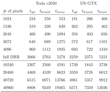
Table 2.3: Impact on kernel performance using rules 1 and 2 described in sub- section2.3.2. Kernel execution times are average of 100 executions and the unit µs. Columns topt present execution times of kernels using all rules. Columns t_branch present execution times of kernels using all rules but rule 1. Columns t_linear present execution times of kernels using all rules but rule 2.

Tesla c2050 570 GTX

# of pixels t_opt t_branch t_linear t_opt t_branch t_linear

1024 234 258 553 181 206 408

1536 319 339 639 263 295 462

2048 466 490 1094 358 403 656

3072 648 689 1275 572 617 1101

4096 969 1112 1935 693 722 1310

full DRR 2666 2763 5278 2259 2375 5221

10240 2307 2560 4591 1739 1843 3738

20480 4469 4539 8623 3359 3728 6012

30720 6515 6971 13766 4961 5357 9912

40960 8808 9249 19465 6571 7359 13026

The results of the first two rules are presented in Table 2.3. The missing branching optimization resulted in a 6-13% performance decrease, 8% in average if the optimized version is considered 100%. The linear memory caused a 1.75- 2.4 times slowdown consequently on both GPUs based on the Fermi architecture nearly independent from the block size and number of threads.

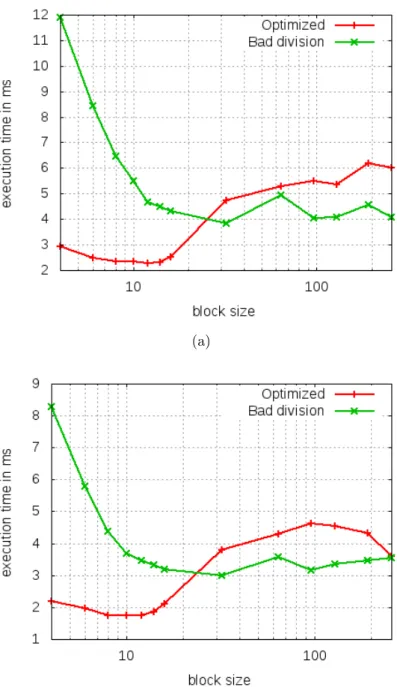
Rules 3 and 4 can be measured effectively only together so, in the following these rules are covered together with the block size dependence of the execution time. In Figures2.6-2.13 the execution time dependence of division pattern and block size on Tesla C2050 GPU and GTX 570 GPU. Both GPUs show similar characteristics. First of all, the gain is 2.3 if the best result of the optimal kernel is compared to the best result of the kernel with bad division pattern in the case of 1024 threads. This ratio is in the range of 1.92-2.36 on the Tesla C2050 GPU

(36)

and in the range of 1.75-2.25 on 570 GTX GPU.

From 1024 to 3072 threads (see Figures2.6-2.9) the performance of the kernel using the unoptimized division pattern is lower or equal to the optimized kernel independently from the block size. These are the cases when the SMs of the GPUs are not filled completely. However, these are the cases that are used in 2D-3D registration in most cases.

In the case of larger number of threads there is a range where the bad division pattern performs better than the optimized one provided the same block size is used (see Figures 2.10-2.13). The reason is as follows. In all cases the execution time is built up of two dominating components and the block size has completely the opposite effect on them. The first component is the pack of division operations in the first part of the algorithm and the second one is the repetitive texture fetch operation in the main loop. If the block size increases the effectiveness of the divisions increases as well (see the identical nature of the first part of the green lines in Figures 2.10-2.13). In case the block size decreases to the optimum the effectiveness of the texture fetch with this reading pattern increases. The weight of the two component is different in the case of the optimized division pattern compared to the unoptimized division pattern, the execution time curve is shifted as well. Since the weight of the divisions decreased in the case of the optimized pattern the direction of the shift is towards the smaller number of threads in a block.

My previous results showed similar characteristics [32] on two additional hardwares with older compiler and driver. These results are presented in Table 2.4 and referenced in Table 2.1.

On 8800 GT GPU optimal block size is 8 in all cases. The increase of the execution time with respect to the optimal execution time is in the range of 57,3−116,8% the mean of the increase is 82%. On 280 GTX GPU optimal block size is 8 in all cases. The increase of the execution time with respect to the optimal execution time is in the range of 8,3−27% the mean of the increase is 18.7%. On Tesla C2050 GPU optimal block size varies from 10 to 16. The increase of the execution time with respect to the optimal execution time is in the range of 5− 23%, the mean of the increase is 9.3%. On 580 GTX GPU optimal block size varies from 8 to 16. The increase of the execution time with

(37)

(a)

(b)

Figure 2.6: Execution time dependence on division pattern and block size n the case of 1024 threads. On the x axes there is the block size and the y axes is the execution time inms. Red curve corresponds to mean of measurements applying all rules, while green curve corresponds to measurements applying only rules 1 and 2. (a) Shows characteristics in the case of Tesla C2050 GPU. (b) Shows characteristics in the case of 570 GTX GPU.

(38)

(a)

(b)

(39)

(a)

(b)

(40)

(a)

(b)

(41)

(a)

(b)

Figure 2.10: Execution time dependence on division pattern and block size in the case of 10240 threads. On the x axes there is the block size and the y axes is the execution time in ms. Red curve corresponds to mean of measurements applying all rules, while green curve corresponds to measurements applying only rules 1 and 2. (a) Shows characteristics in the case of Tesla C2050 GPU. (b) Shows characteristics in the case of 570 GTX GPU

(42)

(a)

(b)

(43)

(a)

(b)

(44)

(a)

(b)

(45)

(a) 8800 GT (b) 280 GTX

(c) Tesla C2050 (d) 580 GTX

Figure 2.14: Large thread numbers (40960) on 8800 GT, 280 GTX, Tesla C2050, and 580 GTX in the case of the Pig dataset. The execution time of the optimized kernel is depicted as a function of the block size. The results of the four GPUs can be seen. It is clear that the best block size is in the range of 8-16. This is an unexpected result since the physical scheduling of threads is made in warps (32 threads).

(46)

Table 2.4: Optimized execution characteristics on old compiler and driver [32].

Columns ‘t_o’ represent the means of optimized execution times of DRR computing kernel in µs. Columns ‘bs’ show optimized block sizes for device and thread number pairs. Columns ‘SU’ present speedup of execution times compared to naive block size of 256.

8800 GT 280 GTX Tesla c2050 580 GTX

# of pixels to bs SU to bs SU to bs SU to bs SU

1024 1257 160 1.12 547 96 1.61 417 10 2.44 297 8 2.44

1536 1588 10 1.25 826 160 1.3 510 14 1.97 342 16 2.07

2048 2128 14 1.37 1144 12 1.1 690 32 1.45 391 16 1.78

3072 3016 8 1.34 1480 8 1.3 886 32 1.92 550 192 1.21

4096 3922 10 1.56 1922 10 1.32 1159 64 1.57 700 128 1

6144 5815 16 1.59 2641 10 1.51 1508 64 1.64 1006 192 1.3

8192 7300 32 1.09 3424 10 1.36 2222 128 1.31 1290 256 1

full ROI 5269 128 1.34 4545 32 1.31 3989 128 1.1 2666 128 1.17

respect to the optimal execution time is in the range of 8.2−14.8% the mean of the increase is 11.1%.

2.5 Discussion

In this Chapter, 4 rules are presented that proved to be an essential aid to optimize a fast DRR rendering algorithm implemented in C for CUDA on more contemporary Nvidia GPUs. Furthermore, a significant new optimization parameter is introduced together with an optimal parameter range in the presented case. The presented rules include arithmetic, instruction and memory access optimization rules as well. The performance gain is presented corresponding to the 4 rules as well as to the block size. For thread numbers required to the registration (1024-3072) all rules caused performance gain independently from the block size. However, outside this interval, gain from the division pattern vanishes and changes to loss if the block size is not taken into account together with the division pattern. Namely, for the same block size the execution time is better in the case of unoptimized division pattern than in the case of optimized division

(47)

pattern (see rules 3-4 in Section 2.3.2). It is illustrated in Figures 2.10-2.13. A likely explanation is given for this phenomenon in Section2.4.

I have showed through several experiments that the block size is an important optimization factor and I have given the interval (between 8 and 16) where it resides in nearly all cases for randomly sampled DRR rendering independently from the hardware. These optimized values differ from values suggested by the vendor in nearly all cases. Additionally, the same interval has been determined with similar characteristics on an old compiler and driver combination on two other older GPUs as well. This indicates that this characteristic is independent from the compiler and the driver and it is an intrinsic property of the NVIDIA GPUs. Further measurement data is provided in the Appendix C.

The ray cast algorithm is embarrassingly parallel: the pixels are independent from each other and similarly, integrals of all disjoint segments of a ray are independent too. Another advantage of the algorithm is its independence from the pixel and virtual X-ray source locations. The performance bottleneck of the algorithm is its bandwidth limited nature. For each voxel read instruction there are only four floating point additions. There are possibilities to improve even further the execution time. Line integral of disjoint segments can be computed independently. This enables the complete integral of one pixel to be calculated by one or more blocks. A block works on a segment that can be either the complete line inside the volume or a fraction of it. In the case of full ROI DRRs the block and grid size can be chosen to be 2D, so a block renders a small rectangle of the ROI. This arrangement may be more effective, since the locality is better than in the 1D case, which was used in this work. Completely different approaches can not be much faster in the random case because rendering is bandwidth limited.

The presented results outperform a similar attempt from the literature [31,30].

The comparison is easier to the work of Dorgham et al. [31]. In one case nearly the same (8800 GT and 8800 GTX) and in another the same (580 GTX) GPUs were used. Both the 3D data and the number of rendered pixels are in the same range (512×512×267 vs 512×512×72 in the case of 3D data and 512×267 vs 400×225 in the case of number of pixels). Furthermore, the GPU compiler and driver is assumed to be the same because of the date of the publication. After normalizing by the ratio between the 3D data and the number of pixels a 5.1

(48)

times speedup appears in the case of 8800 GT GPU and 1.81 times speedup in the case of 580 GTX GPU [32]. If different compiler and driver is allowed than the result of Dorgham et al. on 580 GTX can be compared to the the result of 570 GTX GPU (see Table2.3) normalized with the number of SM-s. The speedup is 2.33.

The comparison to the work of Gendrin et al. [30] is hard since, we have only implicit information on the speed of the DRR rendering. It presents an on-line registration at the speed of 0.4-0.7s. However, the 3D CT volume is preprocessed by (a) intensity windowing (b) and the unnecessary voxels are cut out. The windowing eliminates pixels under and above proper thresholds and maps the voxel value to a 8 bit range. Furthermore, not only the ROI is remarkably smaller than in our case but the projected volume as well. Unfortunately, there is no precise information about the reduced volume size making the exact comparison hardly possible.

2.6 Conclusions

Execution time optimization is in the heart of real time applications. Finding optimization rules and optimal parameters is a non-trivial task. I showed that the rules I defined are indeed effective optimization rules in several important and relevant cases on more GPU hardware. I emphasized the effect of block size on the performance. Furthermore, I determined its optimal range for the DRR rendering. Of course, these results should help in any other cases when the task contains calculation of random projection.

To automatically register the content of an X-ray projection to a 3D CT, 20-50 iteration steps are required. For each iteration, 10-20 DRRs are computed depending on the registration procedure. On the whole this amounts to 200-700 DRRs to be rendered for a registration to converge. DRR rendering is the most time consuming part of the 2D to 3D image registration. Following the presented implementation rules, the time requirements of a registration process can be decreased to 0.6-1 s if full-ROI DRRs are applied. If random sampling is used the time requirement of registration can be further reduced to 0.07-0.5 second resulting in quasi real time operability. This achievement allows new services and

(49)

protocols spread in the practice in the fields where real time 2D to 3D registration is required like patient position monitoring during radiotherapy, device position and trajectory monitoring and correction during minimally invasive interventions.

The code-base was integrated into a prototyping framework of GE. As for my last information the company considered the possibility to use the module in later upcoming softwares.

(50)

Chapter 3 Initial condition for efficient

mapping of level set algorithms on many-core architectures

This Chapter is organized as follows. Section 3.1 summarizes the related work.

Section3.2 describes the interface propagation in an introductory level and presents the fast LS method of Shi. Section 3.3 gives the necessary definitions and tools to handle rigorously the theoretical results presented in Section 3.4. It is followed by Section3.5 presenting the proofs of the Theorems. This part of the dissertation focuses on the initial condition and its impact on the evolution in both theoretical and practical ways. The theoretical part is covered in Sections3.4and 3.5. The context of the practical side is laid down in Section3.7 namely it shows the conventional and the proposed initial condition families. This Section helps to understand the significance of the results. Section3.6describes the two hardware platforms namely, a mixed mode CNN-UM implementation and a GPU, that executed the two case studies described in Section3.8. This Section also presents some examples of the Theorems and demonstrates a segmentation example. It is followed by Section3.9 comparing the Shi LS evolution against a numerical PDE approximation in three cases using different force fields. Section 3.10 gives the discussion and Section3.11 concludes this Chapter.

The use of Level Set (LS) based curve evolution has become an interesting

(51)

research topic due to its versatility and accuracy. These flows are widely used in various fields like computational geometry, fluid mechanics, image processing, computer vision and material science [6]. In general, the method entails that one evolves a curve, surface or image with a partial differential equation (PDE) and obtains the result at a point in the evolution.

There is a subset of problems where only the steady state of the LS evolution is of practical interest like segmentation and detection. In this Chapter, only this subset is considered. In addition, I do not form any operator or force field (F) for driving the evolution of the LSs. However, two theoretically worst case bounds of the required number of iterations are proposed to reach the steady state for a well defined class of LS based evolution. These bounds depend only on the initial condition. Furthermore, the bounds only allow an extremely small number of iterations if the evolution is calculated with a properly chosen initial condition.

These kinds of evolutions are calculated very quickly on many-core devices.

The subject of this Chapter is both theoretical and practical. The theoretical side is clearly two new Theorems in the worst case of the required number of iterations of the LS evolution of [45]. This evolution omits the numerical solution of the underlying PDE and successfully approximates it with a rule based evolution. It is based on the sign of the force fields (F) normal to the curves to be to change. Theorem1gives a general bound and Theorem2assumes a special kind of discrete convexity defined in Section3.3.

The practical side is presented through two case studies, namely, the LS evolution of Shi can be mapped in a straightforward way on two completely different many-core architectures. With a lot of small curves in the initial condition, which would be unfeasible on a conventional single core processor, the proposed The- orems ensure small number of iterations. Additionally, with the change in the initial condition (instead of one curve, a lot of small curves are used) the computing width of the many-core platform is utilized.