RACER data stream based array processor and algorithm implementation methods as well as their applications for parallel, heterogeneous computing architectures Ádám Rák

(1)

RACER data stream based array processor and algorithm implementation methods as well as

their applications for parallel, heterogeneous computing architectures

Ádám Rák

A thesis submitted for the degree of Doctor of Philosophy

Scientic adviser:

György Cserey, Ph.D.

Faculty of Information Technology and Bionics Péter Pázmány Catholic University

Budapest, 2014

(2)

Acknowledgements

I thank Interdisciplinary Technical Sciences Doctoral School of Pázmány Péter Catholic University, Faculty of Information Technology and Bionics, and its senior masters, Professor Dr. Tamás Roska, and Professor Dr. Péter Szolgay for the encouragement and advisement during my studies.

I would like to thank György Cserey, for his support, encouragement, advices and inspiration.

I thank my colleagues for their advices and with whom I could discuss all my ideas: Gergely Balázs Soós, Gergely Feldhoer,

Ákos Tar, József Veres, Balázs Jákli, Norbert Sárkány, Gábor Tor- nai, Miklós Koller, István Reguly, Csaba Józsa, András Horváth, At- tila Stubendek, Domonkos Gergely, Mihály Radványi, Tamás Fülöp, Tamás Zsedrovits, Csaba Nemes and Gaurav Gandhi.

I thank Vida Tivadarné her patience and devoted work to make the administrative issues much easier, the help of PPCU's dean's oce and the help of academic and nancial department.

The support of grants Nos. TÁMOP-4.2.1/B-11/2-KMR-2011-0002 and TÁMOP-4.2.2/B-10/1-2010-0014 are gratefully acknowledged.

I am grateful to Anna for providing her friendship and our discussions even her always busy schedule.

I am very grateful to my mother and father and to my whole family who always believed in me and supported me in all possible ways.

(3)

Abstract

This dissertation (i) describes polyhedron based algorithm optimization method for GPUs and other many core architectures, describes and illustrates the loops, data-ow dependencies and optimizations with polyhedrons, denes the memory access pattern, memory access eciency ratio and absolute access pattern eciency, and presents problem decomposition; (ii) introduces a new data stream based array processor architecture, called RACER and presents the details of the architecture from the programming principle to the applied pipeline processing; (iii) presents a new algorithmic approach developed to evaluate two-electron repulsion integrals based on contracted Gaussian basis functions in a parallel way, provides distinct SIMD (Single Instruction Multiple Data) optimized paths which symbolically transforms integral parameters into target integral algorithms.

(4)

List of Figures

2.1 (a) Geometric polyhedron representation of loops in the dimensions ofi, j loop variables. (b) Another example, 2D integral-image calculation, where data-ow dependencies are represented by red arrows between the nodes of the polyhedron. The dependency arrows point in the inverse direction compared to the data-ow. . . 17 2.2 Polyhedrons can be partitioned into parallel slices, where parallel

slices only contain independent parts of the polyhedron. For an example, rotating the polyhedron depicted in Figure 2.1(b), an optimized parallel version can be transformed. . . 18 2.3 Schematic overview of the steps we need to take before we can

apply geometric polyhedral transformation for optimization. . . . 21 2.4 Polyhedron representation of the dot-product example (a). Re-

arranging the parentheses in associative chains gives a possible solution for its parallelization (b). . . 22 2.5 Scheduling polyhedron nodes to the time×core plain. In the rst

step we place horizontal and vertical barriers, which segment the plane into groups (a). The horizontal barriers are synchronization points of the time axes, so they separate dierent parts of the execution in time and the vertical barriers separate the core groups.

In the next step microschedule the inside the groups to obtain the nal structure (b). . . 24 2.6 Typical coalescing pattern used on GPUs, where the core or thread

IDs correspond to the accessed memory index . . . 28

iv

(8)

LIST OF FIGURES v

2.7 (a) A simple coalesced memory access pattern. (b) Random memory access aided by cache memory. (c) Explicitly using the local memory for shuing the accesses in order to achieve the targeted memory access pattern. . . 29 2.8 Run times of an 8192×8192 matrix transposition algorithm are

depicted on NVIDIA GPU architectures. In the Full-coalesced case I use local memory to achieve coalescing for memory reads and memory writes at the same time. The other two cases are naive implementations, where either the reads or the writes are coalesced only. In the case of Tesla C2050 there is a noticeable improvement which is thanks to the sophisticated and relatively large caches on the NVIDIA Fermi architecture. The NVIDIA GTX780 contains further improved caching which reects of the benchmark times. . 30 2.9 Top and left macroblock dependence of the intra coded blocks due

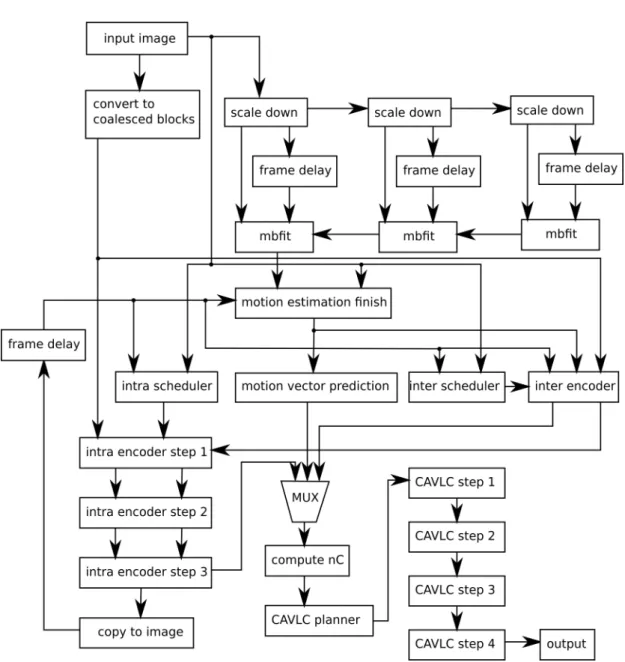
to the in-frame prediction . . . 33 2.10 Data-ow diagram of the GPU implementation of the H.264 video

encoder . . . 34 2.11 Data-ow diagram of the lossy encoding part of the GPU imple-

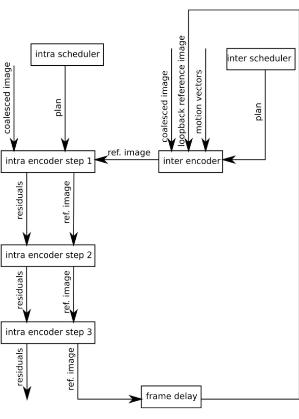
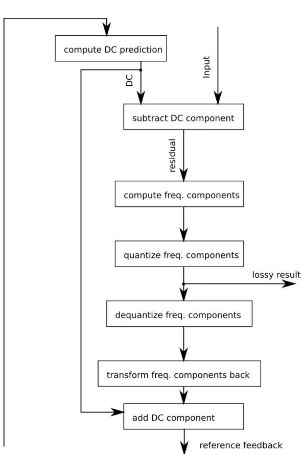
mentation . . . 35 2.12 Data-ow diagram of the non GPU adapted version of the intra

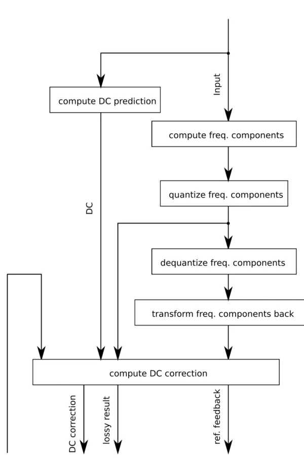
encoder. The reference feedback, which causes the dependencies, loops all the blocks, so the they cannot be factored out of the dependency. . . 39 2.13 Data-ow diagram of the GPU adapted version of the intra en-

coder. The new feedback loop uses DC correction instead of the reference image inside the intra computation, this way most of the computation is free of dependencies. . . 40 2.14 The results of the benchmark of my GPU implementation built

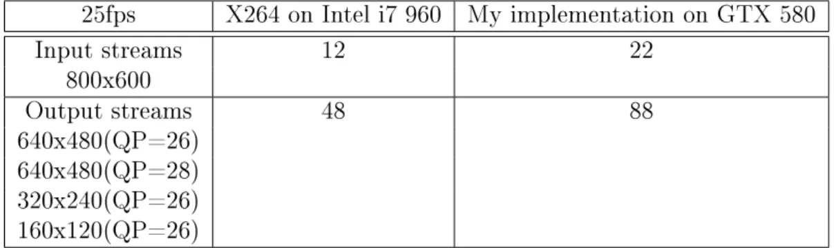
into a live video transcoding system compared to the CPU implementation. The inputs stream were decompressed, rescaled and re-encoded into dierent resolutions and image qualities. . . 41

(9)

LIST OF FIGURES vi

2.15 The results of the benchmark of my GPU implementation built into a live video transcoding system compared to the CPU implementation. The inputs stream were decompressed, rescaled and re-encoded into dierent resolutions and image qualities. . . 41 3.1 The main functional blocks of the RACER computer architecture

can be seen. The architecture includes a central processing unit (RCPU), memory units (MU), periphery units (PU), control unit (RCU) and instruction stream router unit (ISRU). The units of the architecture are connected to each other through the RCPU. . 52 3.2 The program stream which consists of the instruction stream and

the data stream divided into data elements, and the disassembly stream. . . 52 3.3 A simple data stream processing example is shown, where the addi-

tion of two data streams from dierent sources is realized element- by-element by an adder operator realized in the RCPU. The width of data streams can be 4×32 bits, but this parameter can vary depending on the hardware implementation. . . 54 3.4 The computation of Figure 3.3 realized on RACER architecture.

The addition of the rst and second data channel of the input data stream is computed, and the result is placed in the rst channel of the output data stream. Of course the RCPU can perform more complex operations, too . . . 55 3.5 Illustration of the RACER memory, it sorts the information by

tags. In this sorting process one of the channels of the data stream contains the indexes. These indexes are related to the data elements of the data stream, which the SPU arranges by their indexes and it creates the corresponding output data stream. . . 56

(10)

LIST OF FIGURES vii

3.6 Structure of the RACER MU with the communication paths. The RACER MU contains a memory processing unit (MPU) for comparing the data elements. This MPU can be an ALU or an FPU, it should have at least minimally adequate computing capability for data sorting, and is controlled by the memory control unit (MCU).

The MCU receives and executes the related parts of the instruction stream. The MU also includes a data link controller unit (DLCU), which is connected through the data bus to a port of RCPU, where the data transmission can be implemented. . . 58 3.7 Internal structure of the RACER central processing unit. This de-

vice contains the block of processing elements and the data routing elements. The processing elements are connected to the neighbors and are able to process operations on program streams based on the instruction stream. The role of the data routing elements enables the passage of the stream to the processing elements. The processed data stream can leave to the RACER memory or other peripheries through the input/output communication ports. . . . 60 3.8 Internal connections of the RACER CPU, the structure is black,

the connections are gray. These connection gates provide the passage of the data stream between processing elements and data routing elements, between data routing elements and between processing elements. . . 61 3.9 A simple algorithm routed on the RACER CPU. Grey depicts the

used elements. The data streams pass through the data routing elements and processing elements. The processing elements perform calculation operations on the data streams. The data streams merge into one data stream in the junction, which leaves the RCPU through the output port. The data streams are displayed by their traversed routes. . . 63

(11)

LIST OF FIGURES viii

3.10 The internal structure of the processing element of the RACER architecture is depicted. The processing element includes an input multiplexer (input MUX) capable of processing the input of the ports, a local memory connected to the input MUX, a local processing unit (LPU) connected to the output of the input MUX, and an output multiplexer (output MUX) connected to the output of the LPU, providing the output of the processing element. . . . 65 3.11 The internal structure of the FPU without pipeline stages. The

FPU contains a multiplier unit, two comparative units (compara- tors) and an adder unit, which are connected to each other. . . 67 3.12 The internal structure of the FPU with pipeline stages. The multi-

plier, the adder and also the comparison unit comprises more than one pipeline stages. Pipeline registers, that are suitable to store data elements, are assigned to the pipeline stages of the processing. 68 3.13 Connection of two consecutive pipeline stages for half-speed mode.

The feedback plays an important role in controlling when the data propagates, and it eectively enforces the half-speed operation. . . 71 3.14 Timing diagram of a single pipeline stage during normal operation.

It can be seen that data transfer speed is half of the clock speed because of the half-speed operation. . . 71 3.15 The pipeline control cycles through various states during the op-

eration of the pipeline . . . 72 3.16 The state table of a single pipeline stage for half-speed mode. The

state change only happens when the inputs trigger it, otherwise it remains the same. The Data Input is copied to the Data Output, and is latched till it is cleared by the rising edge on the Feedback Input. . . 72

(12)

LIST OF FIGURES ix

3.17 The algorithm of the Mandelbrot-set calculation implemented on RACER computer architecture. The branches or logic operations are depicted by rectangles or squares and are implemented by processing elements. Depending on the design of the processing elements, more than one logic operations can be implemented by one processing element. The feedback streams depicted by lled triangles have priority in the junctions. Without giving priority of particular feedback data streams deadlock occurs and the data streams would be waiting for each other. In data merging junctions, a data stream arriving from a triangle depicted branch has priority to be processed while a stream arriving from the other branch has to be waiting. . . 76 3.18 The possible implementation of the Game of Life cellular automa-

ton rule processing is depicted in RACER graph representation. . 81 3.19 The local tiling for 3 ×3 neighborhood with delay elements on

RACER architecture is depicted. The delay chains receive three inputs from the MUs corresponding to the three consecutive lines, and generate the whole 3×3 tile from it. . . 82 4.1 MD PRISM algorithm consists of a set of interrelated pathways

from shell-pair data to the desired brakets. It consist of the McMurchie- Davidson recurrence relations and contraction steps. Every possible path from the shell-pair data to the (ab|cd) braket format represents a possible solution of the integral problem. Depending on the degree of contractions and the angular moments walking dierent paths can result in dierent run-times. The PRISM meta algorithm tries to the nd the ideal path. . . 96

(13)

4.2 HGP PRISM algorithm consists of a set of interrelated pathways from shell-pair data to the desired brakets. It consist of the Head- Gordon-Pople reuccrence relations and contraction steps. Every possible path from the shell-pair data to the (ab|cd)braket format represents a possible solution of the integral problem. Depending on the degree of contractions and the angular moments walking dierent paths can result in dierent run-times. The PRISM meta algorithm tries to the nd the ideal path. . . 97 4.3 The structure of the BRUSH meta algorithm. All possible paths

are merged together into a graph. The algorithm includes the MD-PRISM and HGP-PRISM transformation steps along with my symbolic transformation steps. The left C_L and rightC_R contraction steps are depicted in the Figure. In the branches for partially uncontracted brakets the contraction step is missing, since it is a trivial identity transformation. . . 99

x

(14)

Chapter 1 Introduction

In recent years a new direction has started in the world of computing, which is based on increasing the number of cores and execution units rather than the clock frequency of the processors. This trend is manifested in all of the network devices, desktop computers and even in cell phones. The main reason for this can be traced back to physical laws, as the miniaturization of microchips and the increase of the clock frequency led to a much too long communication time between the remote parts of the processor. This delay is caused mostly by wiring and metal connections of the chip. The further increase of the clock frequency is therefore not only impeded by a limit determined by the silicon's switching speed, but it also increases the experienced value of the delay. Too much delay implicates more fragmentation of the architecture into several execution units and cores.

According to Moore's law, the manufacturing cost of digital integrated elec- tronics per transistor is becoming cheaper. This will help the above mentioned direction further, as in a well-designed multiprocessor system, the increase of the number of cores is a simple task. This way not only more and more transistors, but more and more cores (or, raw computing power, increasing at the same rate as dened in Moore's law) are gained for the same price.

This trend is lead by graphics processing unit (GPU), which is achieved and even exceeded the number of 5760 cores per microchip in 2014. These multi- core or many-core systems are DSP, FPGA, CELL and GPU, but this trend encompasses the embedded, multimedia processors too.

1

(15)

2

Besides the rapid development of the hardware, the question arises how these architectures can be programmed eciently. Many-core processor systems show not only more variety than traditional predecessors, but require fundamentally new programming approach. In order to integrate as many cores as possible in a processor unit, the computational units were simplied as much as possible.

Practically most of the results of the last twenty years had been thrown away from single processor core optimization. Which focused on a single processor core optimization. Thus the dierence between a simple computational unit, e.g.

Floating-Point Unit, and a core with full functionality is not clear. The functional dierences between many-core and traditional processors are illustrated by that if a strict serial program has been executed on a many-core processor, then the running time is often 100 times slower than running it on a non-parallel CPU.

The standard OpenCL programming language has been created to program such a new parallel systems. OpenCL is a low level C language, which pushes o the problem of parallelization of the algorithms to the programmers.

The ecient implementation of an algorithm requires the deep knowledge of the target architecture. Based on experiences, this knowledge is necessary even while using OpenCL language because the smallest optimization solutions can be speed up the program by a few orders of magnitude. The problem is even more complicated, because the manufacturer (NVIDIA, AMD-ATI) changes its architecture in every year and fundamentally redesigns it in every two years.

Moreover it is common that the manufacturer has diculties to understand its own product and exploit its advantages.

There is signicant demand to have solutions that can automate the parallel implementation of algorithms with mathematically backed methods. This includes those methods too, where implementing algorithms eciently on a new architecture is assisted by machine learning.

Considering these problems, my aim was to analyze the parallelization of general algorithm classes and demonstrate my results and methods on a few dicult algorithms.

The trend is obvious, the number of cores per processor will increase exponentially in the next ve-ten years. However, the dierence between each, following

(16)

3

architectures is not only the number of processors, but the changes of architectures. This evolution leads not only to higher number of processing units, but to the more ecient and optimized operation and also to the increased computational power per area. If we examine the parallel architectures, we nd that the objective is to maximize the general purpose computing power per unit area by employing trade-os. These trade-os and disadvantages at the most common architectures are the following:

The diculties of memory reading and writing of CPUs are hidden by using traditional cache hierarchy. This solution, especially if we have more processor units, increases untenable the ratio between chip area of cache memory and chip area of pure computing. It is a good balance for the less computationally intensive tasks, but quite wasteful in case of scientic or graphical computations.

DSP: digital signal processor. These devices are very similar to CPUs, the dierence is mainly between their parameters. DSPs are designed for running signal processing algorithms eciently (FFT, matrix-vector operations) with low power consumption and competitive price. The chip area (ie. the cost of manufacturing) is much smaller than CPUs', because of the above reasons, DSPs has less cache memory. Therefore the system memory access patterns of DSPs is more restricted if we want to exploit the available bandwidth.

The vector based SIMD (single instruction multiply data) architecture of GPUs (graphical processing unit) introduces a very strong constraint on the implementation of threads. In a workgroup every thread has to do the same operation on dierent data, reading the data from adjacent memory. Therefore both the memory bandwidth and computing resource utilization of the silicon area are very high. But working with this architecture the programmer has to solve the ecient use of memory, contrary to the CPU, this system does not hide the architecture details and does not solve the related problems.

Cell BE (cell broadband engine): this is a hybrid architecture, which includes a classic PowerPC CPU processor connected to SPUs (synergistic processing units).

The SPUs are very simplied vector processing units, which have relatively large local memory on chip. The programmers are responsible to solve even every tiny technical problems, from the appropriate feeding of the pipeline to organize the

(17)

4

internal logic of the memory operations. This device has only indirect memory access via the local memory.

FPGA (eld programmable gate array): On this architecture, arbitrary logic circuit can be implemented within certain broad limits. Usually the implemented circuit is relatively ecient, since the desired circuit is realized physically on the FPGA by connecting on-chip switches. Consequently the logic circuits of the FPGA can be adapted directly to the given task, therefore this architecture can exploit most eciently the available processing units. However the cost of this enormous exibility is the low density of the processing units on the chip surface, since the switching circuits and universal wiring need large chip area.

Systolic Array: this classical topological array processor architecture contains eectively only execution (computing) units, adder and multiplier circuits, which are usually solve some linear algebra operations in parallel. Its applicability is very limited, because its topology is specic for the executed algorithm. This architecture does not contain neither memory architecture, nor program control structure. These units should be provided by another system. The exibility is sacriced for eciency, since the computing units utilized almost 100 percent- age during operation and the surface of the silicon chip contains eectively only computing units.

CNN (cellular nonlinear/neural networks): this architecture is ecient at using local image processing operations (low resolution image processing algorithms on grayscale images) with extremely high speed and low power consumption. Ev- ery pixel is associated to a processing unit, the process is analog and there is only a very little analog memory. Accessing the global memory compared to the internal speed is very slow and also needs the digitalization of the pixels. This architecture is optimized for 2D topological computations with low memory.

Considering these problems, my aim was to design a computational architecture (RACER architecture), which is not limited by the disadvantages of the previous parallel architectures, Turing complete and fully general algorithms can be implemented eciently on it, moreover its performance per area is maximized as much as possible.

The dissertation is organized as follows. Chapter 2 describes polyhedron based algorithm optimization method for GPUs and other many core architectures, de-

(18)

5

scribes and illustrates the loops, data-ow dependencies and optimizations with polyhedrons, denes the memory access pattern, memory access eciency ratio and absolute access pattern eciency, and presents problem decomposition.

Chapter 3 introduces a new data stream based array processor architecture, called RACER and presents the details of the architecture from the programming principle to the applied pipeline processing. Chapter 4 presents a new algorithmic approach developed to evaluate two-electron repulsion integrals based on contracted Gaussian basis functions in a parallel way, provides distinct SIMD (Single Instruction Multiple Data) optimized paths which symbolically transforms integral parameters into target integral algorithms. Chapter 5 summarizes the main results and highlights further potential applications, where the contributions of this dissertation could be eciently exploited.

The author's publications and other publications connected to the dissertation can be found at the end of this document.

(19)

Chapter 2 Polyhedron based algorithm

optimization method for GPUs and other many core architectures

This chapter introduces a new method of a compiler application to many-core systems. In this method, the source code is transformed into a graph of polyhedrons, where memory access patterns and computations can be optimized and mapped to various many core architectures. General optimization techniques are summarized.

2.1 Introduction

The multi-core devices like GPUs (Graphics Processing Unit) are currently ubiq- uitous in the computer gaming market. Graphical Processing Units, as their name implies are used mostly for real-time 3D rendering in games which is not only a highly parallel computation, but also needs great amounts of computing resources. Originally, this need encouraged the development of massively parallel thousand core GPUs. However these systems can be used to implement not only computer games, but also other topological, highly parallel scientic computations. Manufacturers are recognizing this market demand, and they are giving more and more general access to their hardware, in order to aid the usage of GPU for general purpose computations. This trend has recently resulted in relatively

6

(20)

2.1 Introduction 7

cheap and very high performance computing hardwares, which opened up new prospects of computationally intensive algorithms.

New generation hardwares contain more and more processing cores, sometimes over a few thousand, and the trends show that these numbers will exponentially increase in the near future. The question is how developers could program these systems and may port already existing implementations on them. There is a huge need for this today as well as in the forthcoming period. This new approach of the automation of software development may change the future techniques of computing science.

The other signicant issue is that GPUs and CPUs have started merging for the biggest vendors (Intel, NVIDIA, AMD). This means that developers will need to handle heterogeneous many core arrays, where the amount of processing power and architecture can be radically dierent between cores. There are no good methodologies for rethinking or optimizing algorithms on these architectures.

Experience in this area is a hard gain, because there seems to be a very rapid (≈3 year) cycle of architecture redesign.

Exploiting the advantages of the new architectures needs algorithm porting, which practically means the complete redesign of the algorithms. New parallel architectures can be reached by specialized languages (DirectCompute, CUDA, OpenCL, Verilog, VHDL, etc.). For successful implementations, programmers must know the ne details of the architecture. After a twenty years long evolution, ecient compiling for CPU does not need detailed knowledge about the architecture, the compiler can do most of the optimizations. The question is obvious: Can we develop as ecient GPU (or other parallel architecture) compilers as the CPU ones? Will it be a two decade long development period again or can we make it in less time?

Every algorithm can be seen as a solution to a mathematical problem. The specication of this problem describes a relationship from the input to the output.

The most explicit and precise specication can be a working platform independent reference implementation, which actually transforms the input from the output.

Consequently, we can see the (mostly) platform independent implementation, as a specication of the problem. This implicates that we can see the parallelization

(21)

2.1 Introduction 8

as a compiling problem, which transforms the inecient platform independent representation into an ecient platform dependent one.

Parallelization must preserve the behavior in the aspect of specication to give the equivalent results, and should modify the behavior concerning the method of the implementation. Automated hardware utilization has to separate the source code (specication) and optimization techniques on parallel architectures [9].

The polyhedral optimization model [53] is designed for compile-time parallelization using loop transformations. Runtime parallelization approaches are based on TLS (Thread-Level Speculation) method [54], which allows parallel code execution without the knowledge of all dependencies. Researchers are inter- ested in algorithmic skeletons [52] recentely. Usage of skeletons is eective if the parallel algorithms can be characterized by generic patterns [55]. Code patterns address runtime code optimizations too.

There are dierent trends and technical standards emerging. Without the claim of completeness, the most signicant contributions are the following: Open- MP [16] - it supports multi-platform shared-memory parallel programming in C/C++ and FORTRAN, practically it adds pragmas for existing codes, which direct the compiler. OpenCL [66] - is an open, standard C-language extension for the parallel programming of heterogeneous systems, also handling memory hierarchy. Threading Building Blocks of Intel [17] - is a useful optimized block li- brary for shared memory CPUs, which does not support automation. One of the automation supported solution providers is the PGI Accelerator Compiler [18]

of The Portland Group Inc., but it does not support C++. There are application specic implementations on many-core architectures, one of them is a GPU boosted software platform under Matlab, called AccelerEyes' Jacket [20].

Overviewing the growing area, there are partially successful solutions, but there is no universal product and still there are a lot of unsolved problems.

2.1.1 Parallelization conjecture

My conjecture is that any algorithm can be parallelized, even if ineciently. This statement disregards the size of the memory, which can be a limiting factor, but serial algorithms suer from the same problem too, so this is still a fair

(22)

2.1 Introduction 9

comparison. In order to dene this statement in a mathematically correct way, I need a simple denition of the parallelization potential of non-parallel programs.

For easier mathematical treatment we can disregard the eect of limited global memory of the device.

Given ∀P₁ non-parallel program, with the time complexity Ω(f(n)) > O(1), let us suppose that ∃P_M ecient parallel implementation on M processors with the time complexity O(g(n))where:

M→∞,n→∞lim f(n)

g(n) =∞ (2.1)

This means that given big enough inputs, where the input size is n, and an arbitrary huge number of core, we can achieve arbitrary big speedup over the serial implementation of the algorithm. From Equation 2.1 we can derive a practical measure of how well an algorithm can be implemented eciently on a parallel system:

η(M) = lim

n→∞

f(n)

g(n) η(M)≥O(1) (2.2)

In case of arbitrary big input sizen, we can achieve only a speedup limited by the number of cores. I call this speedup η(M), which is a function of the number of cores the architecture has. This limit depends on both the implemented algorithm and the architecture, so η(M) can be called parallelization eciency. It can describe in an abstract way how much the implemented algorithm is parallelization friendly. It can be seen that achieving practical speedup is equivalent to η(M)>O(1). Consequently if η(M) =O(1) then the problem is not (eciently) parallelizable so, Equation 2.1 does not hold.

Some brute-force algorithmic constructions for many-cores yield inecient speedup, for example Equation 2.3, which means that the measured speedup of the algorithm is the square root of the number of parallel cores.

η(M)≥√

M (2.3)

(23)

2.1 Introduction 10

This limit is very arbitrary, but in my opinion anything lower than √ M speedup is not economical, because this scales very well for small architectures, where the number of cores is below 16, like CPUs, but is very impractical for GPUs, where the number of cores is measured in thousands.

I can state that anything with a parallelization eciency less than √ M is practically not parallelizable in the many-core world, however that is why I chose the lower limit of my conjecture to be √

M.

2.1.2 Ambition

Parallelization is a very dicult and potentially time consuming job if done man- ually. Fully automating it is a computationally impossible task, but even partially automating it, on a set of algorithmic classes can greatly increase the productivity of the human programmer.

My aim was to describe algorithms using a general mathematical representation, which enables us to tackle the algorithm parallelization more formally, and hopefully more easily. I used polyhedral geometric structures to describe the loop structure of the program, which is used in modern optimizing compilers for high level optimizations. However, it was unable to represent more complicated dynamic control structures and dynamic dependencies inside loops, so I had to extend the theory to encompass a wider range of algorithmic classes.

In a static loop, we know everything about the control-ow behavior of the loop in compile time, this can be easily extended by allowing the loop bounds to be known just before the start of execution of the whole loop structure [22, 23].

A dynamic loop, or control-ow, in the other hand cannot be known in compile time, every decision in the code happens in run-time depending on the results of the ongoing computations.

While the classical polyhedral approach covers many useful algorithms, it can be very lacking in practice, because the lack of dynamic control handling. My ob- servation is that by just including a few more very constrained algorithmic classes containing dynamic control can practically cover most useful cases, especially if we only consider GPU programming. This approach simplies the original dif- cult problems into tting the algorithms into these classes, after that we have

(24)

2.2 Polyhedrons 11

recipes for implementing these classes on the given architectures.

2.2 Polyhedrons

Because computation time generally concentrates in loops, it is practical to depict the algorithm as a graph of loops, where the graph represents the data-ow between the dierent loops. These loops are the hot points of the algorithm and we can run them on parallel architectures for better performance. Hot point means that most of the execution time is concentrated inside them. This is a very general way of porting algorithms, but there are numerous issues with this approach that I aimed to mitigate.

When we execute an algorithm on a parallel architecture, it usually boils down scheduling loops on cores. This in practice means, that we try to map the parallel execution onto the parallel hardware units, in both space and time. In order to optimize and schedule them better, we can convert loops into polyhedrons. This allows a mathematical approach where each execution of the core of the loop is a single point of the polyhedron, because (well behaving) loops are strictly bounded iterative control structures. This mapping between discrete geometric bodies and loops is a straightforward transformation if possible.

Discrete polyhedra can be dened multiple ways with linear discrete algebra.

I dened these loop polyhedra as generic lled geometric shapes in a discrete euclidean space bounded by at faces. The exact denition can vary by context in the literature. My denition is as follows:

Points: x¯∈N^d Bounding inequality system: M·

x¯ 1

≥¯0 whereM ∈R^(d+1)xn Points of the polyhedra:P:=

¯ x

M· x¯

1

≥¯0

F_{f ilter}^Π :=P→ {true, f alse}

Kkernel :={∂R1...∂Rn,S, ∂W}

(2.4)

Denition 2.4 denes the polyhedron corresponding to a loop structure. The polyhedron contains points of a ddimensional space of loop variables. The given

(25)

2.2 Polyhedrons 12

matrix inequality denes a convex object in this space. All points of this convex object are part of the polyhedron, these points dene set P.

In the denition,x¯is a point of the polyhedron, matrixMdenes the faces of the polyhedron. In the algorithm x¯ corresponds to each execution of the core of the loop structure, and Mcorresponds to the bounds of the loops. These bounds can be linearly dependent on other loop indexes, which allows us to rotate and optimize the polyhedron.

It is desirable to allow minimal dynamic control-ow in this formalism, so I have dened F_{f ilter}^Π , which is a scheduling-time executable function to decide the subset of polyhedron nodes that we would like to execute. This means that this function is quasi static in the sense that it had to be decided just before we start to execute the loop structure, but we do not know the result of this function before that. If we run a scheduler before the loops, to map them into parallel execution units, we can use this F_{f ilter}^Π function to lter out the polyhedral nodes early. This way we can prevent the scheduling of empty work to the execution units. It is important to note that ltered non-functional parts should be in minority, otherwise the polyhedral representation is useless for optimization, and it is processing a sparsely indexed structure instead of an actual polyhedron.

The K_kernel represents the kernel operation to be executed in the nodes, this is the formal representation of the core of the loop structure. I treat this code as sequential data-ow, which has memory reads at the start, and writes at the end.

In Denition 2.4 ∂_R1...∂_Rn are the memory reads, Sis the sequential arithmetic, and ∂W is the memory write. If we cannot t the extra control-ow inside the kernel into our representation, we can treat the rest inside as data-ow function S, but any side eects should be included in the memory operations ∂_R, ∂_W.

Because of the possibly overlapping memory operations, internal dependencies arise, and possibly between polyhedrons too. We depict dependency set asDwith the following denition:

(26)

2.2 Polyhedrons 13

D:={f_i|f_i :P→P} f_i(¯x) :=round

D_i·

x¯ 1

where D_i ∈Q^(d+1)xd F_{f ilter}^D :=DxP→ {true, f alse} Dependency condition

f_i(¯x)can be evaluated at scheduling-time in O(1) time

(2.5)

Dependency set is a function which maps from nodes of the polyhedron to nodes of the polyhedron. In practice, it denes that a given node of the polyhedron depends on which nodes must precede it in execution time. A dependency set can be dened as multiple maps. Most algorithmic cases can be covered by a linear dependency mapping, which can be represented as a linear transformation on the index vector.

Dependencies arise from the overlapping memory operation, mostly because one operation uses the result of another one, or less likely they update the same memory and one overwrites the output of another.

The domain of Matrix D is rational numbers, this allows more general transformations, so we can represent most dependencies by a linear transformation.

In simple cases it is an oset, but it can be a rotation as well, e.g. the swap (or mirror) of the coordinates. Most of the time linear transformations should have enough power of representation, because the original algorithms are created by human intelligence, and these loops tend to have linear dependencies, otherwise it would be too dicult to understand.

In practice however, there are dependencies which are dynamic/conditional and can only be evaluated during execution time. I propose the formal treatment of dynamic dependencies, in the case where we can evaluate them no later than the start of the loop structure containing the mentioned dependency. It is possible since the dynamic dependencies, like the previously mentioned F_{f ilter}^Π lter function, are constraints on the scheduling, and we are doing scheduling just before executing the loops. This is the reason why the dynamic behavior of dependencies is treated as F_{f ilter}^D lter function, which is very similar to the F_{f ilter}^Π kernel lter function. This F_{f ilter}^D function represents the dynamic part, it is essentially a condition which states which dependencies on which nodes should be counted as valid.

(27)

2.2 Polyhedrons 14

In the following I dene the memory access patterns similarly to dependencies.

The access pattern maps from the nodes of the polyhedron to the memory storage indexes.

A single memory access∂ in the kernel is described in the following:

∂R, ∂W :read and write operations g :P→Nⁿ

g(¯x) :=round

A· x¯

1

where A∈Q^(d+1)xn

(2.6)

Where a member of Nⁿ is an n dimensional memory address, and g(¯x) is the access pattern.

It is interesting to note that the memory can be n dimensional as well. Al- though the memory is usually handled as a serial one dimensional vector, in some cases it can be a 2D image mapped topologically into a 2D memory. While the memory chips are 2D arrays physically, they are addressed linearly from the processing units. However, GPUs have hardware supported 2D memory boosted by 2D coherent cache in order to help the speed of 3D and 2D image processing. Therefore it is useful to manage higher dimensional memory. It is even more practical from a mathematical point of view since, the polyhedra made from loops tend to be multidimensional, we can make the memory access pattern optimizations much easier if we can match the dimensionality of the memory indexing to the polyhedron.

The similarity between the denition of access patterns and dependencies is not a coincidence as I have mentioned previously, overlapping or connected memory operation can imply dependencies. However, the importance of access patterns does not stop here, because most architectures are sensitive to memory access. Some architectures can only do very restricted memory access patterns, like FPGA, or systolic arrays. Others are capable of general random access, like CPUs and GPUs, however the bandwidth dierence between access patterns can be over an order of magnitude. It is very important to optimize also this practical aspect, because such bandwidth dierences matter greatly in engineering practice.

(28)

2.2 Polyhedrons 15

2.2.1 Handling dynamic polyhedra

It was mentioned in the previous section that the most important part of this work is formalizing the handling of dynamic polyhedra, which includes both conditional execution and conditional dependencies. When we process static loops we generate a walk of polyhedron o-line. This walk essentially implies an optimized loop structure and perhaps a mapping to parallel cores. Generating a walk however is not possible for dynamic polyhedra, because essential information is missing at compile time.

The obvious solution is generating the walk in runtime, which can have a performance drawback. In extreme cases this can take longer than the actual computation we want to optimize. My solution to mitigate this problem is that we do not need to process everything in execution time. All the static dependencies can be processed oine, and the dynamic dependencies can be regarded as worst cases in compile time. This in itself does not solve the original problem, but opens up the avenue to generate code for the scheduler. The job of this scheduler is to generate the walk during runtime, but due to the knowledge we statically know about the polyhedron, this scheduler code is another polyhedron itself. Our aim is to make the structure of the scheduler simpler, and hopefully less dynamic like the original problem, because otherwise this solution would be an innite recursion.

In practice this means that the schedule should be somewhere halfway between an unstructured scheduler and a fully static walk. In order to avoid confusion with the static walk, I am calling the dynamic walk Plan. This name is more bet- ting, because in the implementation the Plan contains only indexes, instructing which thread should process which part of the polyhedron.

The unstructured scheduler in this context means that the scheduler cannot eectively use the fact that it is processing a polyhedral representation. It is a simple algorithm which iterates through each point of the polyhedron, and schedules them when their dependency is satised. This can be greatly improved if the scheduler only looks at the possible cases, by using the static information.

Since the Plan governs the order of the execution, it determines the access patterns of the physical memory, this implicates that the formalism should include

(29)

2.2 Polyhedrons 16

this relationship as well. The following Plan related notations and denitions are used in this paper: Plan (see Equation 2.8): P(Π) is an optimized dynamic walk of the polyhedron. It is the job of the scheduler to generate this before the execution of the loop structure, after that the loop structure is executed according to this Plan.

Plan eciency (see Equation 2.9): η(P) is closely related to parallelization eciency. It well characterizes the hardware computing resources according to the plan, according to the pipeline and computing unit utilization. In other words if all the pipelines are optimally lled in all compute units (cores), we can say that this eciency is1. We can dene this eciency as a ratio of available computing resources and the computing resources used by when we execute the Plan.

Access pattern (see Equation 2.10): ∂(P,Π) depicts the memory access pattern of the polyhedron while it is using the Plan.

Access pattern eciency: η(∂(P,Π)) characterizes the eciency of the utilization of the hardware memory bandwidth. This is similar to the Plan eciency, but instead of computing resource, we have memory bandwidth.

2.2.2 Loops and data-ow dependencies in polyhedra

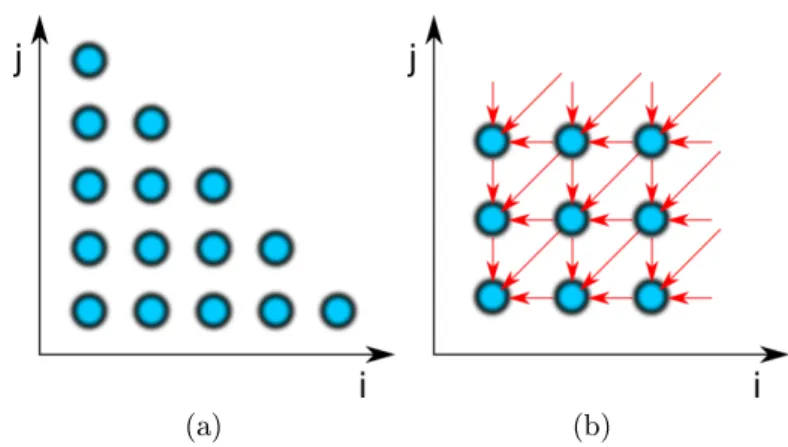
In this section I would like to present two examples in order to aid the under- standing of the concepts behind polyhedral loop optimization. The rst example is a loop with two index variables i, j, which can be represented by a discrete polyhedron depicted in Figure 2.1(a):

for ( int i =0; i <5; i++) for ( int j =0; j <(5−i ) ; j++) { S1( i , j ) ;

}

The polyhedron is two dimensional, because there are two loop variables and it is a triangle because the bound of the second variablej is dependent on the rst i. There are no dependencies depicted, and the core of the loop is represented by an S1(i, j) general placeholder function.

In the following I would like to present a more realistic example:

(30)

2.2 Polyhedrons 17

(a) (b)

Figure 2.1: (a) Geometric polyhedron representation of loops in the dimensions of i, j loop variables. (b) Another example, 2D integral-image calculation, where data-ow dependencies are represented by red arrows between the nodes of the polyhedron. The dependency arrows point in the inverse direction compared to the data-ow.

for ( int i = 0 ; i < n ; i++) for ( int j = 0 ; j < m; j++) { int sum = array [ i ] [ j ] ;

i f ( i > 0) sum += array [ i −1][ j ]; i f ( j > 0) sum += array [ i ] [ j−1]; i f ( i > 0 and j > 0)

sum −= array [ i −1][ j−1]; array [ i ] [ j ] = sum ;

}

This example presents an integral-image calculation, where the algorithm cal- culates the integral of a 2D array or image in a memory-ecient way. The equivalent polyhedron can be seen in Figure 2.1(b) where the dependencies are depicted by arrows, which is practically the same as the indexing of the memory reads.

It was chosen because this polyhedron has a complicated dependency and access pattern, which will serve as a good example optimization target later.

While the rst example does not benet from polyhedral optimization, as it can be easily parallelized anyways, the second example will be examined in depth in the next section.

(31)

2.2 Polyhedrons 18

Figure 2.2: Polyhedrons can be partitioned into parallel slices, where parallel slices only contain independent parts of the polyhedron. For an example, rotating the polyhedron depicted in Figure 2.1(b), an optimized parallel version can be transformed.

2.2.3 Optimization with polyhedrons

The polyhedral representation of the loops provides a high level geometrical de- scription where mathematical methods and tools can be used. Ane transformations can be applied on polyhedrons. These approaches can be used for multi-core optimizations. Polyhedrons can be partitioned into parallel slices, where parallel slices only contain independent parts of the polyhedron and they can be mapped to parallel execution units. For an example, rotating the polyhedron depicted in Figure 2.1(b), an optimized parallel version can be transformed, see Figure 2.2.

These rotations can be easily done by polyhedral loop optimizer libraries [24], but the rotated/optimized code is not presented here because the resulting loop bound computations are of little interest for the human reader.

Geometric transformations can be used to optimize the access patterns too, not just the parallelization, because they transform the memory accesses along the polyhedron. These transformations should be done o-line (compile time) even for dynamic polyhedra, because there is usually no closed formula for getting them. However, in this optimization we search for an optimal ane transformation in the sense that it should allow the highest bandwidth while still obeying the dependencies and the parallelization. This is a general constrained discrete optimization problem, and thanks to the low dimensionality, we can easily aord to solve this by a genetic algorithm, or random trials, if we have an accurate

(32)

2.2 Polyhedrons 19

model of the architecture.

If we want to handle dynamic polyhedra, we need to compute the worst case for the dependencies while we try to nd a parallelization, and later on, in execution time, we use the transformed polyhedra in the scheduler. In this scenario, the complexity of the scheduler can be greatly reduced, because the problem has been reduced in the o-line optimizations. A practical example would be if the dependencies in Figure 2.2 were actually dynamic. In this case the parallelization is the same, but for some nodes the dependencies are missing. This is an optimization opportunity because we can possibly execute more nodes in parallel, so the scheduler can look to the next slice if there are available nodes. Thanks to the o-line transformations, the scheduler only needs to look at the polyhedra in (the compile time determined) parallel slices, which greatly simplies the algorithm. Even more, as previously mentioned the structured way of the scheduling algorithm means that it is in itself a regular loop structure, which can optimized the same way.

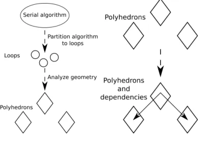
2.2.4 Treating optimization problems

If we need to do high level polyhedral optimizations on real-world algorithms, we need to complete several steps depicted on Figure 2.3 and explained in more detail below. Most of these steps can be done automatically for well behaving algorithms, but some need human intelligence, especially to ensure that we chose the most well behaving realization of the algorithm to analyze.

I have identied the most common steps of this process:

1. Take the most natural, and the least optimized version of the algorithm This is very important to help the formal treatment of loop structure, because the more optimized the algorithm, the more complicated its loop structure tends to be, which can hide many aspects from the optimizations.

2. Consider the algorithm as a set of loops and nd the computationally complex loops

This step can be done semi-automatically, with static code analysis and benchmarking, most compilers already support this (GCC, LLVM)

(33)

2.3 Problems beyond polyhedrons 20

3. Represent the problem as mathematical structures (polyhedra)

This is a bijective mapping between loop structures and polyhedra, a purely mathematical transformation.

4. Discover dependencies in-loop and between loops

Loop dependency tracking is relatively simple after we formalize the loops, there is at least partial support for this already in GCC and LLVM.

5. Eliminate as many dependencies as possible

Some of the trivial dependencies can be eliminated automatically, but most of them need a human hand. We need this step, because dependencies prevent parallelization and constrain the transformations, limiting out the ability to optimize.

6. Quantify Π, ∂,P

We formally quantify the shape of the polyhedra, the memory operations and their implied dependencies, and the possible ways for scheduling the loops.

7. Find the best transformation for parallelization

This is a static polyhedral optimization (we disregard the dynamic parts), there are useful solutions in the literature [21, 25].

8. Estimate speed based onη

We can estimate the speed by the simulation of the transformed algorithm, so we can guess our eciency.

9. Optimize: transform Π, ∂,P to increase speed

We apply geometric transformation to the polyhedra, in order to increase the eciency of parallelization, and memory access.

2.3 Problems beyond polyhedrons

Of course, not every problem has a corresponding polyhedron representation, which can be transformed easily and automatically into parallelized form. There

(34)

Figure 2.3: Schematic overview of the steps we need to take before we can apply geometric polyhedral transformation for optimization.

are a number of cases, which need human creativity to nd appropriate solutions or sometimes we do not even know any eective solutions for them. In the following, two such examples are presented.

2.3.1 Dot-product, a simple example

Let us examine the simple dot-product example in the following code comparing to its polyhedron representation in Figure 2.4(a).

r e s u l t = 0 ;

for ( int i = 0 ; i < n ; i++)

r e s u l t += vector1 [ i ]∗vector2 [ i ] ;

Unfortunately, there is no usable polyhedral transformation available here.

In this example, data-ow dependencies force a strict order of the execution.

These dependencies are connected through an associative addition operator. So the solution of this problem here is to rearrange the order of the associative operators, see Figure 2.4(b), which will create the well known parallel reduction.

(35)

(a) (b)

Figure 2.4: Polyhedron representation of the dot-product example (a). Rear- ranging the parentheses in associative chains gives a possible solution for its parallelization (b).

2.3.2 Irreducible reduction

We often encounter more complex algorithms, for example reduction, where the transformation is not trivial:

x_n+1 =f(x_n, y_n) (2.7)

Where the y_n is the input, and the nal x_n is the output of this general reduction scheme. If thef function is not associative, then we cannot simply use the parallel reduction. In this case, we have to investigate the f function deeply, in order to convert the iteration into a parallelizable representation.

I can state, that my polyhedral transformation, and parallelization methods, can handle the complexity up to the associative operations. This means that if there are dependencies in the polyhedron, it is only possible to break them up, if they are connected by associative operators. More complex dependencies are not breakable, and they can possibly prevent the parallelization. However if the loop structure has enough dimensions, it still might be possible to nd a parallelizable part of the algorithm.

(36)

2.4 High-level hardware specic optimizations 23

2.4 High-level hardware specic optimizations

Computational complexity usually concentrates in loops. Loops can be represented by polyhedrons, these are important building blocks of the program.

Branching parts of the code can be reduced into a sequential code, or sometimes can be built into the polyhedrons, depending on the conditions. After eliminating the implicit side eects, the sequential code can be translated to pure data-ows.

Applying these methods, only a bunch of polyhedrons - connected together in a data-ow graph - have to be optimized. As we have already seen, this is not trivial in itself, but after we have this representation, we can move forward to the optimization problem.

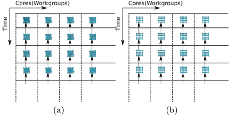
2.4.1 Kernel scheduling to threads

Kernel execution scheduling is a mapping of the polyhedron nodes to the symbolic plane of time × core id. Horizontal and vertical barriers can be dened on this plane. The horizontal barriers are synchronization points of the time axes, so they separate dierent parts of the execution in time and the vertical barriers separate the core groups. Dependencies cross horizontal barriers parallel with the vertical barriers (Figure 2.5). Actually, the most important task of this hardware aware scheduling is to place these barriers. After the barrier separation, the micro- scheduling is usually trivial inside the groups.

The vertical barriers usually represent a physical separation between the computing core groups. In the case of GPUs, it means that the multiprocessors are separated by the vertical lines. It is very important that the dependencies do not intersect the vertical lines, but intersect the horizontal lines. If these forbidden intersections actually happen, then on most architectures we lose the ability to ensure correctness of the dependency, because the hardware usually decides the exact timing of the parallel schedule.

In the groups separated by the barriers, the hardware specic micro-scheduling is executed, which is trivial because we do not have to take into account the dependencies.

(37)

2.4 High-level hardware specic optimizations 24

(a) (b)

Figure 2.5: Scheduling polyhedron nodes to the time×core plain. In the rst step we place horizontal and vertical barriers, which segment the plane into groups (a). The horizontal barriers are synchronization points of the time axes, so they separate dierent parts of the execution in time and the vertical barriers separate the core groups. In the next step microschedule the inside the groups to obtain the nal structure (b).

A Plan is a parallel walk of the polyhedron, dened in the following way:

P(Π) :NxN→ P

(NOP) (2.8)

Indexing of the plan is : P(Π(t, i)) where t is time and iis the core id.

The plan maps the polyhedron to the nodes of a polyhedron. It is possible that this set includes symbolic empty items too, because not all nodes have functional operations. The eciency of a plan can be dened by simply dividing the number of polyhedron nodes by the area of the plane (which is equal with the number of nodes multiplied by time). Obviously the dependencies will limit the maximum eciency.

Plan eciency denes the eectiveness of the usage of computing resources according to the plan:

P(t, i) t∈[1;T] i∈[1;I]

η(P) =

P|Pi|t_P_i T ·I

(2.9)

(38)

2.5 Memory access 25

2.5 Memory access

On a multi-core architecture we need to keep the utilization of both the cores and memory bandwidth at optimal levels. Improving the core utilization has been dis- cussed already in depth in previous sections. In this section the focus is on how to improve the memory bandwidth after we have achieved the parallelization and handled the dependencies. Many-core architectures are less reliant on traditional memory caching, because they cannot put enough cache memory into every core, due to the chip area constraints. Therefore the memory access of each core has to be coordinated in a way which is close to the preferred access pattern of the main memory. This memory is almost aways physically realized by DRAM technology, which prefers burst transfers. Burst transfers are continuous in address space, so when cores are accessing the memory, the parts of the memory accessed by dierent cores should be close to each other. Older GPUs [26] mandate that each thread should access the memory in a strict pattern dictated by their respective thread IDs, otherwise the memory bandwidth is an order of magnitude lower than optimal. Newer GPUs [34, 27] use relatively small cache memories for re- ordering the memory transfer in real-time, consequently we only need to keep the simultaneous memory accesses close together, but there is no dependence between the relative memory address and the thread IDs. These constraints on optimal memory access patterns underline the importance of the access pattern optimization, however even if we look at the traditional CPU cache coherency, we can nd that there are optimizations possible too, if we wish to achieve the maximal performance, so these optimizations are important regardless of the architecture.

2.5.1 Access pattern ( ∂( P , Π) ) and relative access pattern eciency ( η (∂( P , Π)) )

I have formally dened the access pattern including its dependence on the runtime walk of the polyhedron, which is the plan. The access pattern can be seen as a product of the data storage pattern and the walk of the polyhedron. Together these two contain where and when the program accesses the memory.

So we can formally write:

(39)

∂(P,Π) :=∂◦P (2.10)

Where the∂(P,Π)is the access pattern which depends on the parallelization.

2.5.2 Memory access eciency ratio ( θ )

We can write the memory bandwidth eciency as η, which is the ratio of the full theoretical bandwidth and the achieved bandwidth. Usually achieving the theoretical maximum is unfeasible, so we can depict maximal achievable eciency as η_best. Consequently we can depict the lowest possible bandwidth by η_worst, in this case we deliberately force the worst possible access pattern to try to lower the bandwidth of the memory access. We can dene an interesting attribute:

θ:= η_best

η_worst (2.11)

Where θ is the memory access eciency ratio. This number can describe, in a limited way, the sensitivity of the architecture to the access pattern of the memory. Bigger θ usually means that the architecture is more sensitive to the memory access pattern, and we need to be more careful in the optimization. The important limitation of this number is that it does not tell us anything about the access patterns themselves.

2.5.3 Absolute access pattern eciency ( η(∂ (Π)) )

If we want to optimize the access pattern, we can approach the problem from two sides. The rst is to optimize the storage pattern of the data we want to access. This is constrained by the fact that we usually need to access the same data from dierent polyhedra, so the dierent storage patterns may be optimal for dierent places of accesses, but we can only choose one. The second way is to optimize the plans(P), which are runtime walk of the polyhedra. This is done independently from other polyhedra which access the same data, however we are constrained by the polyhedral structure, the parallelization and the internal polyhedral dependencies.

(40)

For easier handling of the optimization, we wish to, at least formally, eliminate the dependence of the access pattern eciency on the plan(P).

Let the absolute access pattern eciency be:

η(∂(Π))≈max

P (η(∂(P,Π))) (2.12)

In other words, the absolute access pattern eciency is the maximal achievable access pattern eciency by only changing the plan(P). This eliminates the dependency on the plan, so the storage pattern optimization can take place.

This denition seems quite nonconstructive, since it implicitly assumes that we somehow know the best possible solution. However, the polyhedral optimization is a relatively low dimensional problem, and the dependencies also constrain it even more, which means that the plan has an even lower degree of freedom, so low that we can even perform exhaustive search. Very often this means searching in one degree of freedom. As a consequence it is aordable to compute η(∂(Π)).

2.5.4 Coalescing

In GPU programming terminology memory access coalescing means that each thread of execution accesses memory in the same pattern as their IDs as depicted in Figure 2.6 and Figure 2.7a. This is usually true for the indexes of the processing cores as well. This coalescing criterion only has to hold locally, for example, on every group execution threads, but not between the groups. This minimal size of these groups is a hardware parameter.

On GPUs coalesced access is necessary for maximizing the memory bandwidth, however for modern GPUs [34, 27] the caches can do fast auto-coalescing.

This means that the accesses should be close together, so the cache can collect them into a single burst transfer for optimal performance.

2.5.5 Simple data parallel access

This is the ideal data parallel access as depicted on Figure 2.7a, where every thread of execution reads and write only once, in other words there is a linear mapping between cores and memory. GPUs are principally optimized for this,

(41)

Figure 2.6: Typical coalescing pattern used on GPUs, where the core or thread IDs correspond to the accessed memory index

because this is very typical in some image processing tasks, e.g. pixel-shaders.

This access pattern is highly coalesced by denition, this can achieve the highest bandwidth on GPUs.

2.5.6 Cached memory access

If the eects of caching are signicant, mostly because they are big enough, we can optimize for cache locality. Consequently we achieve much higher bandwidth than the main memory has, because if our memory accesses are mostly local, and stay inside the cache, they do not trigger actual main memory transfers. However, highly spread-out memory accesses trigger main memory transfers, but due to the logical page structure of the memory, these transfers are even worse, because every transfer triggers a transfer of a whole page to/from the main memory.

The size and bandwidth of the various levels of the cache hierarchy are very important factors, sometimes even more important than the bandwidth of the main memory. All modern CPUs are optimized for this operation, and newer GPUs also contain enough cache, so this might be relevant for them too. This is depicted on Figure 2.7b.

(42)

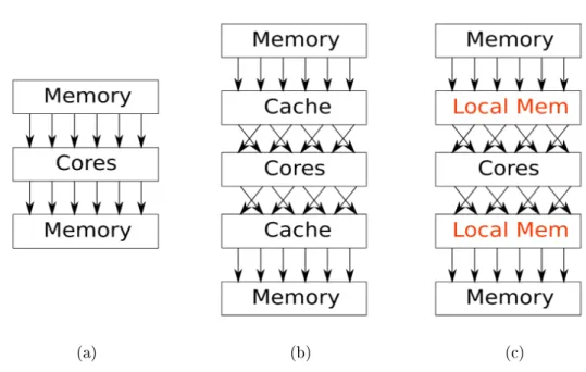
(a) (b) (c)

Figure 2.7: (a) A simple coalesced memory access pattern. (b) Random memory access aided by cache memory. (c) Explicitly using the local memory for shuing the accesses in order to achieve the targeted memory access pattern.

2.5.7 Local memory rearranging for coalescing

Local memory rearranging is a GPU technique for achieving more coalesced memory access as depicted in Figure 2.7c. I would like to emphasize that this optimization can be automatized in my formal mathematical framework, which would ooad a lot of work from the human programmer. Furthermore this is the most important step in linear algebra algorithms implemented on GPUs [28], because complex but regular access patterns routinely arise in these algorithms.

Essentially this is similar to caching, but thanks to the precise analysis based on the polyhedral model we know the exact access patterns. Therefore instead of using general heuristic caching algorithms, we can determine the storage pattern of the data inside the local memory, which would maximize the memory bandwidth. This would always perform signicantly better than caching for rep- resentable problems in this framework. On some GPUs [34] there is enough caching for signicantly speed up the non-coalesced access, this can be seen in Figure 2.8, where run times of an8192×8192 matrix transposition algorithm are