INJECTION GUIDANCE ACCURACY AS APPLIED TO LUNAR AND INTERPLANETARY MISSIONS H.J. Gordon

INJECTION GUIDANCE ACCURACY AS APPLIED TO LUNAR AND INTERPLANETARY MISSIONS

H.J. Gordon1

Jet Propulsion laboratory, California Institute of Technology, Pasadena, Calif.

ABSTRACT

Studies that were performed at the Jet Propulsion Laboratory to determine the accuracy of a typical inertial guidance system as applied to future lunar and interplanetary missions are discussed. Errors in guidance systems are described and analytical techniques for converting these into injection and target errors are presented. The statistics of injection, target, and midcourse maneuver errors are briefly developed.

The determination of midcourse maneuver fuel requirements, which is the primary purpose of the study, is then discussed.

The effect of parking orbits on injection guidance accuracy was evaluated. These parking orbits (circular satellite coast periods) will be necessary for practical space missions of the near future in order to satisfy various geometrical constraints in an efficient manner. The technique for calculating the injection errors and the effect of the parking orbit on these errors is described. The results of studies of several specific trajectories are presented, illustrating the degree of accuracy to be expected for practical deep space missions of the immediate future. It will be seen that parking orbits do not necessarily reduce guidance accuracy, and in fact, that there is an optimum coast arc.

INTRODUCTION

Guidance is necessary in order to steer a vehicle to injection. The guidance system accomplishes this task by determining vehicle position and velocity with some measuring device and controlling the direction of the thrust vector until

Presented at ARS Guidance, Control, and Navigation Conference, Stanford, Calif., Aug. 7 - 9 , 1 9 6 1 . This research was sponsored by NASA under Contract no. NASw-6.

lSenior Research Engineer, Space Guidance Theory Group, Jet Propulsion Laboratory.

the guidance equations are satisfied, at which time thrust is terminated. If the guidance equations are such that all pertur- bations that are sensed are adequately compensated for, the vehicle will follow the equivalent of a standard trajectory unless the guidance equipment is inaccurate. In this case, the only sources of coordinate errors at injection are component errors, which lead to an incorrect computation of vehicle position and velocity. Since the vehicle's path is corrected to compensate for any error, true or false, which the guidance system measures, the coordinate errors at injec- tion can be set equal to the measurement errors. This approach allows a system to be evaluated even though the specific guidance equations are not known. Nonstandard per- formance during burning leads to coordinate dispersions, which are not to be considered as guidance system errors. These coordinate dispersions can be included in the statistical ana,lysis of injection errors, as indicated in the fourth section.2

Guidance system errors can be computed by integrating trajectories with the assumed component errors, or can be derived analytically. This paper derives an analytic method for computing these errors for an inertial guidance

system. The analytic method gives a good first-order approxi- mation that is quite adequate for error studies. By the use of this method a study can be carried out much fasterj requir- ing less computer time than would be needed to actually integrate many trajectories.

DESCRIPTION OF SYSTEM STUDIED

The guidance system postulated for this study is a vehicle- borne gyro-stabilized inertial platform on which are mounted three mutually perpendicular integrating accelerometers. .A digital computer finds vehicle position and velocity and steers to shutoff such that it will compensate for measurable errors in the flight path.

The component error sources considered in this analysis are accelerometer errors and gyro errors. The accelerometer

2The guidance system attempts to compensate for all disper- sions which are sensed. Approximations in the guidance equations may permit some dispersions to be undetected and hence uncorrected. Fuel depletion before desired thrust termination is sensed but leads to dispersions which cannot be corrected. These dispersion sources may be minimized by proper design of the overall system.

errors are considered to be scale factor, null shift, align- ment, and integrator scale factor errors. The gyro errors are considered to be initial offset, random drift and

acceleration-sensitive drift. It is assumed that these error sources are uncorrelated. Fig. 1 shows the accelerometer orientation, Fig. 2 shows one accelerometer computer loop, Fig. 3 shows the gyro orientation, and Table 1 lists the component errors used for this study. These values were taken from the open literature (l-4).3 They represent reasonable values but do not reflect the performance of any specific system.

The pre-injection trajectory is considered to be divided into two powered flight phases, separated by a circular parking orbit coast period. (See Fig. k. ) The parking orbit will be discussed further in the fifth section. The

coordinate errors contributed by each of the powered flight phases are computed in terms of quantities obtained from the

standard trajectory and the results are combined at injection (see Appendix B). Certain assumptions are made in order to simplify the analysis, such that the vehicle is restricted to a plane (the thrust plane).

DESCRIPTION OF COMPUTATION OF INJECTION COORDINATE ERRORS At entry into the parking orbit the position and velocity errors arising from each error source are computed in an inertial Cartesian coordinate system (the plumb line system defined in Fig. 4 ) to obtain a six-dimensional error vector.

The error vectors are transformed to the downrange point where the final burn terminates by a circular orbit Β matrix (see Appendix A ) . This transformation is most simply carried out if the coordinate errors in the plane of motion are first put into polar coordinates (see Fig. k). The total coordinate error vectors at injection are then obtained by adding the errors contributed by the final burn and those accumulated during the coast interval.

Error vectors in Cartesian coordinates are designated by δΧ±

(the subscript i indicates the number of the error source, of which a total of 1 8 are considered). The components of oX± are

designated by Sx î j; j taking on the values one through six, corresponding respectively to δΧ, δΥ, δΧ, δΫ, δΖ, and δΖ which are the displacement and velocity errors defined in the inertial plumb line system. Error vectors in polar coordinates are designated by δΖχ, with elements Öz j _ j, where j takes the values

3Numbers in parentheses indicate References at end of paper.

one through six, corresponding respectively to Δ Χ , O R , Δ Ν , Δ Γ , Δ Ζ , and Δ Ζ · Writing fix^ and oZ± as row vectors, it is con- venient to define [ Δ Χ ] and [ΔΖ] as 1 8 χ 6 matrices with elements ΔΧ-^j and 8z±y

Α [ Δ Χ ] matrix is obtained for each of the two burning periods. These are designated [ΔΧ]χ and [ΔΧ]2 corresponding to the burnout times t^_ and t². The matrices [ Δ Ζ ] ^^{ar e} com- puted from the transformation matrix by: { Δ Ζ ] ^ = LÔXJ^E^, where E^ is the transformation from Cartesian to polar coor- dinates at time t^-, k = 1 or 2 . (See Appendix A. )

The matrix which describes the coordinate errors at injec- tion due to first burn only is [ÔZ]jj_ = [ Δ Ζ] ι Β. For ease of computation, one coordinate error, due to integrator scale factor error, accumulated during the coast interval is cal- culated directly in polar coordinates. This computation results in a [ΔΖ]ο matrix. The total coordinate error matrix at injection is then A = ^ Z ] J J _ + [ Δ Ζ ]2 + ( Δ Ζ ^ . The

elements of these matrices are derived in Appendix B.

STATISTICAL CALCULATIONS

The six injection errors are random variables and must be described by a six-dimensional probability density function.

If each error source is a Gaussian variable, and if a linear relationship exists between these error sources and the injection errors, then the injection error distribution is Gaussian.

An N-dimensional Gaussian distribution can be represented as -1/2

where Xj_ _ are random variables, X = (X]_, X2, ·.·, XN) , the superscript Τ indicates the transpose of the matrix with that superscript, and Λ is the moment (or covariance) matrix which is real and symmetric. The elements of the Λ matrix are the ensemble averages of the products of the elements of the X vector

Λ = ^{" ΧΤΓ =}

1^Λ2 ~1 ^Λ2 ^Λ1 " 3 1 3

σ 2 Ρ

Χ2 2^Λ3 2 ^Λ3

ρ I j.-^

where σ ^ . is the variance of the i^{O n} random variable, and PxiXj is the correlation between the i^h and j^h r andom variables. Thus Λ is a complete statistical description of the probability distribution (5). The moment matrix of error sources Λ on a powered flight trajectory is

(B) _

2

where σSj_ is the variance of the i th error source

(i = 1 , 2 , ···, N ) . The off-diagonal terms are zero because it is assumed that there is no correlation between error sources.

The same technique can be used if error sources are cor-

related, but in practice it is more convenient to use a set of uncorrelated error sources.

By using linear perturbation theory, an error source vector is mapped into an injection error vector by the transformation (using polar coordinates)

Sq = SS L = ( S x , o r , δ ν , δΓ, δ ζ , δ ζ )

L is an Ν x 6 matrix with elements

1 . . = 8q./9s.

= 1 , 2, . .., Ν

= 1 , 2, 6

The moment matrix of injection coordinate deviations ) is then

_^The A matrix, defined in the third section^corresponds to SS L where the elements of S S are the one-sigma values of component errors. Then A1 A = A d ) . It may be desired to add more error sources to the analysis, or to include the effects of coordinate dispersions. This can be done by letting

A*

where Δ is an (N-l8) Χ 6 matrix containing the additional terms to be included in the analysis. Then Λ = A* ^ A* is the required covariance matrix. It is noticed that

Α* Τ A* = ΑΤΑ + Δ^ΤΔ ·

__^If the^U matrix maps injection errors into target errors, δΜ = SqU = (δΜ^, δΜ².· ôMj)- U is a 6 χ 3 matrix with

elements

u. . = 8 M. / A Q .

I J 3 Ι

i = 1 , 2, 6 j = 1 , 2, 3

The moment matrix of target errors is then

=

The elements of M may be position deviations at a standard time or at closest approach, or other quantities of interest such as relative velocity or time of flight at closest approach.

The U matrix may be considered as a function of the initial and final values of some parameter defining position on the standard trajectory. The initial value refers to the point

w^iere gq is evaluated and the final value to the point where δΜ is evaluated. For convenience, the final point may he

considered fixed, as in the previous paragraph in which the definition is given ÔÇL(l) U(l,T) = SK, I indicates injection and Τ the reference position at the target. If a midcourse maneuver is to he made, it will be made at some point C on the trajectory. At that point,

£q(c)

(

>

)

The midcourse velocity maneuver required is then (6)

§q = - SM

= 1 , 2, 3 f. . = eq./8M.

2, 3

such that the velocity components are expressed in the appro- priate coordinate system.

The moment matrix of midcourse velocity requirements is then

A <

- I r i l T = F

A

F

n/- ν

The amount of fuel necessary to perform the midcourse maneuver may then be calculated.

UNITS OF VARIANCE

To determine the effect of each component error, the uncor- rected rms value of the magnitude of the change in impact parameter, which is the distance from the center of the target to the incoming asymptote, was used as a figure of merit, FOM (7)· The components of this FOM are represented by the elements of $~M which have been developed in the foregoing.

δ~Μ = ÖS LU = δ SD where D = LU. The elements of D are

8M, (i = 1 , 2, ..., Ν

d± J d s± ( j = 1 , 2, 3

k=l i,j=l

3 Ν ^{ô χ}2 Ν

k=l 1=1 ^{1 1} i=l

where

2

- Ï •

( ξ ) * ( § ) • ©

The percentage of FOM2 due to the it n error source, to be called the number of units of variance is

n. = i ΙΟΟρ^σ^ J FO:

The value of the i^*1 error source which produces one unit of variance is

D M2

Values of ni are listed in Table 2 for the trajectories studied.

u± = FOM

EFFECT OF PARKING ORBIT

Direct ascent trajectories lose payload rapidly as true ano- maly at injection increases. In order to satisfy the necessary geometrical constraints and avoid large payload losses, the launching location must be moved. This is an impractical solu- tion. By using a parking orbit as part of the ascent trajectory, the launcher is effectively moved, and a given mission may be accomplished with a resulting greater payload. In addition to this primary argument for the use of parking orbits, their use affords a simple mechanism bf correcting for launch time delays ( 8 ) . Thus it appears that a parking orbit will be used for most lunar and interplanetary missions.

A study was made to determine the effect of the parking orbit interval on guidance errors. The parking orbit deter- mines the effects of the errors due to the first burning phase.

The second burning phase errors, in polar coordinates, do not change for a given mission. This illustrates the utility of the polar coordinate system for the near Earth part of the trajectory. For a given parking orbit, the ascent trajectory does not change significantly with launch time delay so that [£Z]l may be considered constant. Then the moment matrix at

injection into the parking orbit, Λ ^¹^ = [ Δ Ζ] ι [ΔΖ]^]_ is also constant. To determine the effect of the parking orbit on the injection errors

ΛΙ) . - ' ^Τ

= A A = ^[$z]± β + [ S Z ]2 ( Δ Ζ ]¹ β + [ S Z ] -1

= [δζ\1 [ Δ Ζ ]

+ β

j [ S Z G [δζ)

+ [ΔΖ]^ [ Δ Ζ ]

Β

+ Β_ ΐ Τ[ Δ Ζ ] ^ [ Δ Ζ )¹ |^Β

where Λ = [ Δ Ζ] ϊ |δ2]2 is the contribution of the second burn phase. A ^¹'²' = 1 δ^]ϊ [ Δ Ζ] 2 Β "1 is a matrix in the form of a sum of outer products of error vectors due to first burn and those of second burn rotated back around the coast arc to the point of injection into the parking orbit. The effect of the parking orbit on guidance accuracy is through the correlations between injection errors which are seen to be functions of the coast arc, through the Β matrix.

When the post-injection trajectory is determined, launching from a given location at a certain time requires a definite coast arc in the parking orbit. For purposes of studying the effect of the parking orbit, it was assumed that the coast arc could be continuously varied for a given mission. This implies moving the launcher location. As previously pointed out such an implication is unrealistic, but it does point out the effects that are caused by the parking orbit. Another way to change the coast arc would be to launch at a different

date, but this requires a different post-injection trajectory, and the effect of the coast interval would not be as clearly seen.

RESULTS

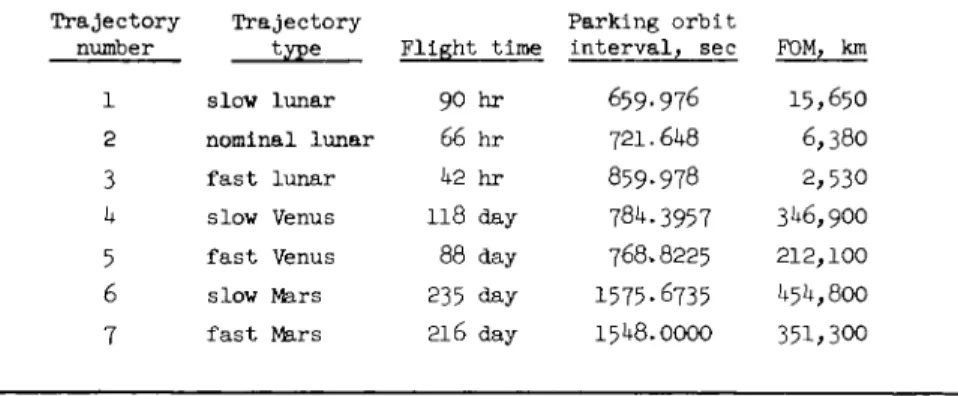
The technique described has been used to determine the FOM for several representative lunar and interplanetary missions.

Table 3 describes the trajectories and the FOM associated with each of them for the system described in the second section with the component errors listed in Table 1. The flow chart

of computations performed is shown in Fig. 5·

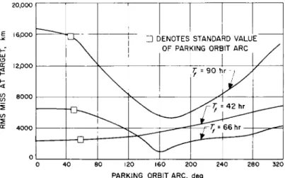
Fig. 6 presents FOM vs. coast arc in the parking orbit φ

for the interplanetary trajectories, and Fig. 7 shows data for the lunar trajectories. It is clear that there is an optimum value of the coast arc This is because correlations between coordinate deviations change as a function of the parking orbit interval, and certain errors may cancel each other.

Table k lists the standard deviations in polar coordinates and the correlation coefficients for the slow lunar trajectory.

Data for the other six trajectories are similar.

Fig. 8 presents the FOM vs. flight time for the three lunar trajectories. These trajectories impact at roughly the same time, thus having similar geometrical properties. It is seen that the faster trajectories tend to have smaller target error

(but, see Fig. 7 where there is a reversal for a coast arc greater than 1 3 2 ° ) . A similar conclusion would be reached for the interplanetary cases. This does not mean that a larger midcourse maneuver would necessarily be required on the slower trajectories, for the higher error sensitivities mean that less correction is required for a given error.

As seen in Appendix B, the values of some of the error terms depend on certain parameters; specifically accelerometer erection angle 0 and gyro orientation angles α and β. These parameters were varied for the fast Venus trajectory, and the results are shown in Fig. 9·

CONCLUSIONS

It is seen from Table 2 that of all the error sources con- sidered, only a few are of major significance. Any improvement in the design of the other components would not improve guidance accuracy much if the major error sources were unimproved.

As shown in Figs, 6 and 7, there is an optimum value of coast arc which minimizes the effects of guidance component errors. By scheduling launches appropriately, trajectories could be designed that would use near-optimum coast arc.

Other considerations, such as post-injection trajectory charac- teristics determined by the positions of the planets will normally determine the scheduling of a launch. The value of the parking orbit study is that it shows that longer coast in- tervals do not necessarily require larger midcourse maneuver capabilities.

As shown in Fig. 9, there is an optimum set of values for the guidance parameters a,β, and φ. This figure applies to a specific trajectory, but a similar result would apply to other trajectories. The method developed in this paper may be used to evaluate the guidance parameters for any specific trajectory.

ο

^ 1

in-

to ο ο

CO Ο Ο

CVJ

o n

•AI

Ö

• H

CVJ

CD Ο U

CVJ

o n

• H en

Ο

CD Ο ο

Ö

• H CD

>

I

CJ ö

• H I CD

CD Ο ο

ο CJ

• H CD

ο

- P

• H - P H

CÖ - P CÖ

> s - P

• H Ο Ο H

£

CD 4 J

• H

CD - P CÖ CD

U

CÖ H

Ο rH

eu

ο

- ρ _{0 H} t>5

(D • H

rH

Ö cd

• H U

+1 _cd -P ^{• H} _{r Q}

rH CÖ

rH rH

cd Ο

W ^{C H}

0 CD

CD rH

CD

~ P CD

Ö • H

CD

Ο <Ö _Ö

CD CÖ

H

- P 0 CÖ

rH >

CD rH

Ο Ν CD

rH - P - P

<4H • H î>i Ö r Q H • H CD rH H Ο Ο ^{CÖ - P}

g ö CD

cd hO ^{• H CÖ}

- P Ö S Ο CD

• H no ^Ο

rn CD

CÖ CD r a H P h • H - P

CÖ P h

TP

JS ^{Ο §>}

CÖ - P • H

rH CD

Ο U

CD - P CD CD r £ Ö r S

- P • H Ο

CVJ

c

rH +

+

CVJ r -

X!

> | rH

H - P

I

+

<3

0 .

O l rH rH I

• H CD

CD Ο Ο

rH CVJ

ο

II

rH

II

- p

Ο

Ο

OJ OJ Ο ^CJ

CD CD

Ω ^W ON ON -P Β

Cm

Lf\

Η Ι—1 X X

Ι Ι Λ

0Λ ON CO Η VO VO

Ο CO ΟΛ ON Η

m <D

- p cö ö

•H Ο Ο Ο

cd

• Η CO

• Η

HL. >

I

Ο

CD

Ο Ο HL >

Ο

OJ

ο

ΟΛ •Ν Ο OJ

OJ Ο-

Ρ Ο

νο

03

ο

CJ

• Η

ω

• Η

Η Ö

Ο

• Η

-Ρ

ο

Ο

ο

Ο Τ-

•HI Ή

χ l>

•Hi Ο

Χ! I Η

•Η I ·Η

•H CO CD -P ÎH

CO ο

CD

•H

ft

Ο

ο

+

Χ I Η

•Η CÖ -Ρ

ΓΗ

•Η

•Ρ

CO CD

•Η -Ρ

•Η -Ρ

·Η| Ο

Χ I Η CO ο

ο ^•Η _CO

2

:>>

Η CÖ CO CO CD

ο

CD CD

~P

ο

+

OJ ·Η χ

CVJ ·Η +

CO CÖ

ί>>

Η ο

-Ρ ο

CD CÖ · Η S

-ρ ω

nd CO Η !>>

CÖ CO

-Ρ CO

ω ΕΗ

APPENDIX B: DERIVATION OF ERROR TERMS

One of the major aims of this analytical derivation is to avoid integrating perturbed trajectories. If the parking orbit interval is changed, the second burn phase produces different incremental Cartesian coordinates, although it pro- duces identical incremental polar coordinates. (The incre- mental coordinates measured are of interest, since they

correspond to the physical situation of setting all initial conditions equal to zero at the start of the second burn. ) With a changed parking orbit interval, the local horizon at start of second burn will have rotated through v/rAr radians with reference to the standard local horizon ( Δγ= θ). The

effect of this rotation can be duplicated by imagining that the accelerometers and gyros have been rotated by this amount and that the second burn occurs at the standard location on the coast arc. Then the transformation [δχ]2Ε2 = [δζ]2 uses the standard E2 matrix. In the following derivations the subscript k takes values 1 or 2 for first or second burn, and

£k = ζ + (k - l)v/rAr, where £ indicates 0, a , or β.

ACCELEROMETER ERRORS Mathematical Model

It is assumed that the accelerometer axes A, B, and C are aligned relative to a fixed inertial reference as shown in Fig. 1 and that the computer loop is as shown in Fig. 2.

Effect of an Accelerometer Scale Factor Error

As may be shown (Fig. 2) the differential equation for the error in the A coordinate due to a scale factor error J^ only is

δλ + - τ δΑ = J A

The solution of this equation is

OA = J A = J (X cos

0

0)

ΔΧ = J^A(X cos²0^k + Y sin 0^ cos

V

ΔΧ = J^A(X cos20k + Y sin 0^k cos Δ Ϋ = δΧ tan 0,

δΥ = δΧ tan 0, Δ Ζ = Δ Ζ = o

Similarly for the Β accelerometer

δχ = J^B(X sin²0^k - Y sin 0k cos 0k)

δχ = J^B(X sin²0^k - Y sin 0k cos 0k) δ Ϋ = -δΧ cot 0k

δΥ = -δΧ cot 0,

and no first-order errors arise from J Effect of a Null Shift Error

As may be shown (Fig. 2 ) the differential equation for the error in A coordinates due to a null shift n^ only is

A + -rr δ Α = η

r^{J A}

The solution of this equation is r³

δΑ = n k T

^The subscript m denotes a measured coordinate, as distin- guished from a true coordinate. It will be assumed throughout that the measured coordinate deviations are equal to the true coordinate deviations.

Therefore the error terms are^"

δΧ = η \ / — cos φ. sin It

δχ ^r3

1 - cos δΫ = δχ tan φ^Λ

rk δγ = δχ tan

0

δζ = δ ζ = 0 Similarly for the Β accelerometer

δχ

δχ = .3

δΥ δγ δζ

-— sin

0,

Β μ ^rk

= -SX cot

0

= -δΧ cot

0

= δΖ = 0

1 - cos

and for the C accelerometer

δΧ = δΧ = ÔY = δΥ = 0

δζ = η_ \ / — sin

δΖ = n ^{c T} O S ^

yj

Therefore the error terms are Τ

Effect of an Alignment Error

As may be shown (Fig. l) the differential equation for the error in the A coordinate due to the A accelerometer only is

Ä = X cos (0. + e. ) + Y sin (0. + € . )

m m ^{v r}k A^/ m ^{v r}k A'

so that, since ^ is a small angle

8K = € (-χ sin d + Y cos 0n )

m Av m rk m rk ' Therefore the error terms are

δΧ = € Λ(-Χ sin φ. cos 0_ + Y cos2 0. ) A^v m ^rk ^rk m ^rk^y δ Χ = * Λ(-Χ sin 0. cos 0 + Y cos2 0. )

Av m rk rk m rky

δΥ = δΧ tan 0R

δΥ = δΧ tan 0,

k

Δ Ζ = Δ Ζ = ο

Similarly for the Β accelerometer

δΧ = € (X cos φ^Λ sin 0, + Y sin2 d ) Bx m rk rk m rk ' ÔX = C (X cos 0. sin 0. + Y sin² 0ⁿ )

B m ^rk ^rk m ^rk^y δΥ = ^{- Δ Χ} cot 0k

δΥ = -δΧ cot 0k

δΖ = ^{Δ Ζ =} 0

The C accelerometer alignment error was considered to con- sist of two components éqx and c^y such that

δ 1

=

c Ä

Assuming that these two components are uncorrelated and have equal standard deviations e~ about zero mean

Therefore the error terms are

δχ = δχ = δγ = δγ = ο Effect of Integrator Scale Factor Error (Clock Error)

This error arises from errors in the timing device that controls the integration interval in the digital integrator.

From Fig. 2, the differential equation for the error in A coordinates due to a clock error (J-^) only is

5Ä + (1 + J^tf δΑ = (2 + J^t)J^tÄ - (1 + J^t)J^tÄ^m r

The solution of this equation is

= <L(2A - A ) to first order

-r v τ η '

δλ = J, (À - À ) to first order' t m

Although all the terms required to evaluate the integrals are available on the standard trajectory, it was found that the first-order approximation is quite adequate for these terms.

Therefore the error terms are

δΧ = J. (X - X )

tv m

δΧ = J, (2X - X )

tv m

δΥ = J, (Y - Y ) tv m7

δ Υ = J (2Y - Y ) t m δ ζ = δζ =

ο

The clock error would also cause a change in the parking orbit interval. This effect, which is that of starting the second burn at the wrong time, can be most easily calculated directly in polar coordinates. It is simply an error in the downrange distance

δχ = - Jtr0 J (t^± + r +Δ0

where r is the parking orbit interval. This element forms the only nonzero element in [δζ]^·

GYRO ERRORS

Mathematical Model

It is assumed that the gyro axes are oriented as shown in Fig. 3· This particular configuration is chosen to eliminate anisoelastic drift rate (i.e., drift rate proportional to the product of accelerations along spin and input axes) while maintaining orthogonality of the input axes. With no

anisoelastic drift, the general expression for angular error θ about the input axis of a gyro is

E = e0 + e0t + ^s/ aTd t - MT/ asd t θ0 = initial offset

0Q = random drift rate

a = measurable acceleration along the input axis

ac = measurable acceleration along the spin axis constants

The gyro error will cause the accelerometers to sense a false acceleration, and the acceleration error vector is

Sa = θ Χ

(standard) ^{É?l θ} 2 ^{0·^}

Χ Υ m m Input Axis Perpendicular to the Thrust Plane IA]_

J 0 X - i θ Y

u m m

i j k S a = 0 0 ⁰

X Y 0 m m

Sx = -γ

• Y 0 . + 0 t - μ^τ J (X cos α +

Y

m O 0 I ^ ^v m m

SY = χ

> 0 ^{+ « 0 *,nt - μ}

" " τ

Γ

0 I _ / Q m m in α) dt

The integral appearing in these two equations must be evaluated as

(k - l)(X^{m l} cos α^λ + Y^{M L} s i n^{e i}) ⁺

't.

cos ÖL + Y sin et ) dt m k m k'

uk-l

where the quantities multiplied by (k - l) represent the acceleration sensitive drift effects of first burn as initial

conditions for the second burn. Setting this quantity, cos a± + Ym]_ sin αχ = W]_, and interpreting the integral to be over the first or second burning phase (for k = 1 or 2, respectively), the error terms are

+* ί l^k ^{c o s a}k + s i n ai r+ <k • l } υ λ ]

δ Χ » -^Ö0^Ymk - *0 [ ^Jlk ^{+ (K - ^ Υ}Γ Π2^ 1 + T +Δ' ) ]

+ "l [^T3k ^{CO S} °k ^{+ X}Uk^{Si n} \ ⁺ (^k " !) ^{Y m 2 W}l ]

δ Υ » V m k + *0 [ *2k ⁺ <k - Χπ Λ + ' + Δ' > ] - "l [^k CO S ak + *6k^{Si n a}k + ^ -1} Xm2^WlJ

δ Ύ » Ö0^Xmk ⁺ *0 Kk ⁺ <^k » W * l ^{+ Γ + A r}> ]

-

τ [^k

k

6 k

(

- D

i]

Δ Ζ = Δ Ζ = 0

w h e r e

h* - Λ

- \ - A

k-1

τ

θν

^{Λ ft -}

2k t, k-1 m

k-1

r \ . . .

I^{Q V} = / Y X dt

3k k-1 ^{m m}

f \ .. .

= Λ

L5k

L6k

"Ik

L2k

3k

LUk

L5k

L6k

X X d t t. m m

k-1

/t, m m k-1

k-1

X f

dt

)X dt"

m

Y X dt t, m m

k-1

. Y dt t, -, m m

k-1

Χ X dt t. , m m

V l

If}

k-1

Spin Axis Perpendicular to the Thrust Plane SA , SA,

Gyro no. 2 is considered, in which the input axis is β deg above the X axis (the analysis for gyro no. 3 follows imme- diately by setting β^} = β + 90 deg).

S A

θ

cos

sin

X Y m m

k 0

β I ö^ m ^{C O S}^ k - \ ^{S l n}^ k )

δΖ = θ⁰(Ϋ^Η cos ß^ - X^m s i n ^^k) ⁺ ö⁰t(Y^m cos ^ - X^m sin/3 ^R)

+ μΑ(Υ cos ß¹ - X sin ß. ) / (X cos β + Y sin θ ) dt

S^v m ^Mk m ^Mk JQ M M

The integral must be evaluated as

( k- 1 ) ( X^{m l} cosß, ⁺Y ^{m l} sin/3,) ⁺

Λ (X m c o s^ k + \ s i n^ k ) d t tk-l

where the quantities multiplied by (k - l) represent the acceleration sensitive drift effects of first burn as initial conditions for the second burn. Setting this quantity, X cos β, + Y ., sin β., = W^, the error terms are

ml ^ 1

d

δχ = δχ = δΥ = δΥ =

ο

δ ί = < VYm k c o e ^k -X m k sinflk)+ θ 0 [ ll k c o s^{â k}

- i 2 k s i n ß^{k +} ( k - l ) ( Ym 2 cos/3²

- Xm 2 Β ί η ά2) ( ΐ ι + r +Δ Γ ) ]+μ5[ ΐ3 1 ζ c o s²ß^k

+ ^ k " ^{i 5}k) C O S ßk ^{S i n ß}k " ^ k s i n 2 ßk + (k - 1 ) ( Y^{m 2} c o s ß² - X^{m 2} s i n ß²) W²j

ml

i n = Y , (t, • t, , ) - Y lk mkx k k-1 ι mk

lk mkv k k-1 7k

where

r

Iτ,, = I Y dt 7k J m

V l

X2 k ~ ^Xm k( tk " V l ) " Xm k

X2 k = Xm A - V l} - ^{2 I}8 k

where >t κ.

X8k - / Xmd t

J 3

k = V

* - Vl> " V

δ Ζ

= *

(

«k

"

m k

^

0 K k

^k

- I^{2 k} sin/3^k + (k - 1 ) ( Y^{m 2} cosß2

- ^Xm2 ^{S i n} Μ* 1 ^{+ Γ + Δ γ} )] ⁺ "s [^X3 k ^{CO s 2} ^k

+ ( l4 k

"

k

^ k

+

( k - D ( Y

The twelve integrals used in the foregoing analysis can be reduced to seven, since, after integration by parts

where

where

where

where

f

"9 k - "k-1

i = i Y² i+k 2 mk

I4 k 2 """lOk

/

I f Y dt

10k *'^tk-l ^m

5 k 2 mk I = i l

5k 2 Ilk

Λ .

Tllk = J Xmd t

\ - l

''"ok YmkXmk ^3k

I6 k ^{= I}1 2 k " ^X3 k

Ι^{η ρ}, = I Y X d t Ι^κ I m m

V l

Thus the integrals 1 ^ , 1^, 1^, 1^, 1 ^ , 1 ^ and 1 ^ are needed, and these can be evaluated in terms of quantities available on the standard trajectory.

ACKNOWLEDGMENT

The author thanks C.G. Pfeiffer of the Jet Propulsion Lab- oratory, C.I.T., for his basic work on error analysis on which this paper is based, and T.W. Hamilton of the Jet Propulsion Laboratory for his development of the units of variance concept 0

REFERENCES

1 Meisenholder, G.W., "An introduction to the operation and testing of accelerometers," TM 33-2, Jet Propulsion Laboratory, CIT, Pasadena, Calif., Oct. 3> i960.

2 Jensen, L.Κ., Evans, B.H., and Clark, R.B., "Evaluation of precision gyros for space boost guidance applications,"

Preprint ΙΙ75-6Ο, ARS Semi-Annual Meeting, Los Angeles, Calif., May 9-12, i960.

3 "Preliminary descriptive material on the GG8001 Β miniature integrating gyro," U-ED ^Qkl Minneapolis Honeywell Co., Minn., Aeronautical Division, March 28, i960.

h "Preliminary descriptive document, GG 177 hinged pendulous accelerometer," U-ED 987Ο, Minneapolis Honeywell Co., Minn., Aeronautical Division, Oct. 6, i960.

5 Noton, A.R.M., "The statistical analysis of space guidance systems," T.M. 33-15.? Jet Propulsion Laboratory, CIT, Pasadena, Calif., June 15, i960.

6 Noton, A.R.M., Cutting, Ε., and Barnes, F.L., "Analysis of radio command mid-course guidance," TR 32-28, Jet

Propulsion Laboratory, CIT, Pasadena, Calif., Sept. 8, i960.

7 Kizner, W., "A method of describing miss distances for lunar and interplanetary trajectories," EP 67U, Jet

Propulsion Laboratory, CIT, Pasadena, Calif., Aug. 1, 1959.

8 Clarke, V. C , Jr., "Design of lunar and interplanetary trajectories," TR 32-30, Jet Propulsion Laboratory, CIT, Pasadena, Calif.', July 26, i960.

Tablé 1 One sigma component errors (assuming Gaussian distribution)

k Description _k

1 A accelerometer scale factor error 5 ^χ ίο-¹* 2 Β accelerometer scale factor error 5 χ ΙΟ"*

3 ^A accelerometer null shift k χ 10 m/sec

k Β accelerometer null shift h χ 10 m/sec

5 ^C accelerometer null shift h ^χ _ο 2

10 m/sec

6 A accelerometer alignment error 0 (See a )

7 ^Β accelerometer alignment error k χ 10 radian

8 C accelerometer alignment error k χ 10 radian

9 Gyro no. 1 initial offset 5 χ 10 radian

10 Gyro no. 2 initial offset 5 ^{χ -1+}

10 radian

11 Gyro no. 3 initial offset 5 χ 10 radian

12 Gyro no. 1 random drift 3 χ 10 ^ radian/sec

13 Gyro no. 2 random drift 3 χ 10 ^ radian/sec

lk Gyro no. 3 random drift 3 χ 10 ^ radian/sec

15 Gyro no. 1 acceleration-sensitive drift 5 χ 10 rad-sec/m

16 Gyro no. 2 acceleration-sensitive drift 5 χ 10 ^ rad-sec/m it Gyro no. 3 acceleration-sensitive drift 5 χ 10 ^ rad-sec/m

16 Clock error 0 (See b )

A accelerometer alignment error is taken to be zero, as it is considered that the A accelerometer alignment defines a reference direction for all other alignments.

b Clock error was found to have a truly negligible effect even when using pessimistic estimates.

OJ LT\ Η OJ ΟΛ ν ο

cd LT\ ΟΛ H Η OJ

CO Η ΙΓλ ο Η Ο ο

• • Ο

v o Η ο ^{- c i} Ο ο ο

ι—1 Η Η

OJ

Η ^{Ι Γ \} VO _{° Q} ο Ο Ο

cd οο OJ ν ο co ο

CO ι—I ο rH ο ΟΛ Η

Ο

.

ΟΛ Η oo ο Η

6

O O

OJ Φ

• H L T\ CO 1^ CO CO ν ο 00

*d ^{cd CO v o} L f \ ^Η Η ^ΟΛ Γ— ο OJ ^Η Ο ^{VO Ο Ο} ο

-P d ^{• •} ο

ω CO ν ο OJ Ο OJ ο

CO > ^{H (—I}

co (U ο

;>> v o Η VO ΟΛ -c± 0J

3

ο p- ^{0 0 O O} Ο ο ο

co _co ö _OJ ^• _{CO 0J OJ Ο} ^{• ο} _0J ^• _ο

Η > ^{O O Η Η}

Ο Η

φ VO 0J VO OJ ν ο ^ -

h ο ^{O O L T \ L f \} 0J co

3 ^{cd OJ ο - CO ι—I h- OJ}

ο ο ^•

OJ p^ ι/λ ΟΛ ο

6

- 3 - Η OJ

φ ο

ΟΛ Η Ο - c t Η Ο Ο

•Η on Η Ο Ο Η 0J

£η 3 ^{H OJ CO ι—1 Ο ο ο}

cd d

.

.

> ^{v o ρ Ο ν ο Η Ο Ο Ο}

6

v o Η OJ

Ο

ω ο ^ΟΛ Ο Ο [>- co

-Ρ ο ^{VO OJ Ο} ο ^οο ο

•Η H CO CO ο ο

d d ^{• •}

.

ρ ο _{CA Η} ^{ρ cô} _H ^{ΟΛ νο H} ο ^OJ ο

Ο

-Ρ Ρ> -Ρ

ω d d d

φ φ φ

Φ Φ ^ς*

n

H Η Η H Η bO W

cd cd Η H Γ—I •Η •Η •Η

OJ Ο ϋ Η Η Η

ω CO d d cd cd cd

φ ο cd

ι—I •Η u u £η *Η

-Ρ Φ U Φ Φ Φ φ φ φ φ

cd ft ^{-Ρ Ο -Ρ Ο -Ρ ?Η -P ?H Ρ> Ρ» Ρ> -Ρ}

En •Η φ ^ Φ ?Η Φ ο Φ Ο φ ο φ φ φ

ε

ε ^ ε ^ ε ε ε ε

Ο Ο Φ Ο Φ Ο ο ^μ ο ο ^{ο ο}

CO £η Φ Φ Φ u u

Φ U Φ ^ φ Φ φ φ φ φ

Η Ο Η Ο Η -Ρ Η -Ρ Η -Ρ Η Η ^ Η Φ -Ρ Φ -Ρ Φ On Φ <Η Φ CH φ ο Φ ο φ ο Ο ϋ ϋ Ο Ο ·Η ϋ ·Η Ο •Η ο ο ^ ο

ο cd ο cd ϋ ,d ϋ Λ Ο ο ο μ ο

cd CH cd CH cd co cd co cd CO cd φ cd φ cd φ

< PQ < pq ο < ^pq ο

Η OJ Ο Ο 1_Γ\ νο 00