TRANSFER FUNCTION DETERMINATION IN THE PRESENCE OF NOISE FOR A SET OF SIGNIFICANT INPUT FUNCTIONS

T H E P R E S E N C E OF N O I S E F O R A SET OF S I G N I F I C A N T I N P U T F U N C T I O N S

B l R G E R Q V A R N S T R O M

Swedish Forest Products Research Laboratory, Paper Technology Department, Stockholm, Sweden

The investigation presented in this paper is of a theoretical nature but is initiated by the following practical problem. A process is given, the transfer function of which is to be determined by use of data recorded during a limited test period. The amplitude of the test signal that may be fed to the process is restricted. There are also noise sources within the process, producing disturbances superimposed on the signals. The problem is to estimate the accuracy by which the process parameters may be determined and to conclude what kind of test signal is preferable.

Westcott [1] has given a very interesting survey of the parameter estimation problem. It should be pointed out that the present problem is different from the one Westcott discussed. Here it is assumed that the process is available for observation for a long time, so that a statistical description may be worked out for stationary noise sources. The period during which a test signal may be applied is, however, limited because the test implies a certain disturbance in the normal operation of the process. For the same reason, the test signal amplitude is restricted.

In the case discussed by Westcott no information about the noise is utilized besides that obtained during the test interval. Westcott also used disturbances as test signals to insure that the process would not deviate from its normal pattern of behavior. Here an artificial test signal is introduced but small enough to serve the same goal.

With regard to the processing of the measured data, unlimited pos­

sibilities are assumed. A n optimal processing procedure will be defined on the basis of a minimum mean square deviation. H o w this procedure may be realized in practice will not be discussed.

B A S I C T H E O R Y

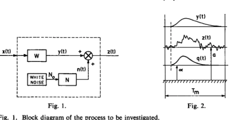
The situation to be discussed here may be represented schematically as a block diagram (Fig. 1). The only available signals, to control and observe, are the input signal Λ:(/) and the process output signal z ( / ) .

α

1 OC

UUI j Π 111 Η Π Ι Tm

NUN

Fig. 1. Fig. 2.

Fig. 1. Block diagram of the process to be investigated.

Fig. 2. Signals involved in the procedure to obtain the process weighting function.

The noise sources within the process are described by a white noise generator combined with a linear passive filter, the weighting function of which is N(u). The noise level is given by the output power of the white noise generator, N⁰ units²/rad/sec. The noise filter output n(t) is added to the unobservable variable y(t). The relation between the latter and the input signal x(t) is assumed to be linear with constant coefficients, expressed by the weighting function W(u) or the corre­

sponding transfer function W(s).

In order to find the function W, we will form a model Q of the process and use a procedure to identify Q and W. The input signal x(t) applied to the process will be fed to the model also, and a com­

parison between the process and the model output will be made. The output difference obtained is a result of the noise source and the mis­

matching of Q and W. The parameters of the weighting function are successively to be varied in such a way that the mean square value of the difference (z — q) approaches a minimum. The function Q corre­

sponding to this minimum will be regarded as the best possible estima­

tion of the process weighting function W.

The time interval at disposal for manipulating the input x(t) and recording the output z(t) is denoted by T^m, as indicated in Fig. 2. The beginning of the interval is chosen as the time t = 0. It is assumed that all transients in the process resulting from input signals prior to that time are negligible. When desirable, we will also put such a restriction on the input x(t) that corresponding transients will vanish before the end of the interval. Thus we are able to repeat the test continuously.

In Fig. 2 the output z(t) is displayed on a level a from the refer­

ence level. In the case where no information from outside the actual interval T^m is available, the level a may be unknown. T o meet this

situation we will introduce in the model Q a parameter α corresponding to the level mentioned.

The other parameters of the weighting function Q(u) will be written as β, γ, δ, etc. Some of these are related to the area of the weighting function, some are unrelated. The area related parameters will interfere with the parameter α in the determination of the level a. T o account for this, we will divide the parameters into two groups, one for area related parameters, represented by β, and the other for are unrelated parameters, represented by y.

The difference (z — q) can be written as follows:

z(t)-q(t) = e(t),

Λ ο Ο

e(0 ⁼ x(t-u)[W(u)-Q(u)]du + n(t)-i-a-oc.

J - 0 0

(1)

The quantity to be minimized by parameter variation is the time average over the interval T^m of the square of the last expression. The presence of noise will make it in general impossible for us to reach the correct parameter values in this procedure, although by definition the procedure is the very best one. The remaining deviation dy of the parameter γ from its correct value is calculated in Appendix I and appears as a result of the following minimizing requirement:

de²(t)/dy = 0. (2)

The bar indicates that the time average of the expression below is to be carried out for the time interval T^m. The deviation rfy as given by eq. (1.8) in Appendix I reads:

This expression (3) is based on the following assumptions:

1. The deviation dy is small so that contributions of an order higher than one may be neglected.

2. Certain conditions of orthogonality are fulfilled (see Appendix I ) or all parameter deviations other than dy are zero.

3. The parameter y is not related to the area of the weighting function or there is no error (α —a) in the zero level of the process output and the model output.

In the case where we have an area related parameter β and are forced to calculate the zero level from the data collected during the

interval T^m eq. (3) above must be modified. Eq. (7) in appendix 1 gives then the deviation.

Eq. (3) tells us the deviation for one particular interval T^m, M o r e interesting is to know a probable deviation or an average value of the deviation for a large number of intervals. The mean value is here zero because of the properties of the noise source chosen. The probabilities of positive and negative deviations of the same magnitude are the same.

A suitable measure is then the mean square value, which is calculated in Appendix I I . Using a bar to indicate a time average the result will according to eq. (2.16) of Appendix I I be:

άγ2 = 4n2kNn Λ ο ο

1*0'

J - o o

ω)

I

The relation is based on Fourier transforms, which is convenient with regard to further conclusions. In the Appendix I I the same for­

mula is also given in the time domain (13). The coefficient k will be considered as a constant indicating the interference between the noise and the measuring signals. For k = 0 there is no interference, and the parameter error is consequently zero. For k = 1 the noise spectrum is flat over the entire range of interest in the measuring procedure and there is a severe noise interference. Eq. (2.17) in Appendix I I gives the following expression for k:

k = f

Γ l*(»|

J ^{- o o} δγ *\Ναω)\2άω

Γ |*0'ω)|

J - o o

dQ(jco) θγ

2

άω

(5)

A L I M I T T H E O R E M

Already from practical experience it is possible to state that there must be a limit with regard to the accuracy by which a parameter can be determined if the test period and the amplitude of the measuring signal are limited. Parseval's theorem (Appendix I I , eq. (2.15)) and eq. (4) offers an opportunity to express the ultimate accuracy in a closed form for the case k=l. Assuming that the largest permissible signal amplitude is a, Parseval's theorem gives us the following inequality:

x(t)<a.

T o obtain a parameter deviation as small as possible we have to make the following integral, denominator of eq. (4), as large as possible.

l * ( » |

GO'ω)

dy

2

dm Max. (7)

For a fixed value of the integral (6), it is directly possible to indicate the character of the input signal giving the maximum value of the integral (7). This input signal should have all energy referred to the frequency domain located at the maximum value of \dQ/dy\. It is ob­

vious that a situation where the input signal has the maximum energy a2 Tm (32) and at the same time all energy located at frequencies cor­

responding to \dQ/dy\^max is a very special case. But this situation gives us a lower limit of the parameter error for all possible input signals.

Using eq. (6) and introducing the maximum value of (33) as discussed here, we get the following formula for the root mean square value Δ γ of the parameter deviation dy:

Α γ > ν - - Ϋ 2 π / , ^{Ϋ Ν} ^ . (8)

This expression has the nature to be expected. The parameter error depends on a noise to signal ratio, the noise being that part of the original noise that cannot be filtered out during the test interval T^m and the signal represented by its maximum value a. The parameter error also depends on the extent to which the parameter affects the transfer function.

A P P L I C A T I O N S

T o illustrate the significance of the preceding formulas, we will apply them in a very simple case using a set of input functions commonly utilized. The process is the simplest possible, a first order time lag, characterized by the following functions:

W(t) = (A/T)e-^t/T, I W(j<o) = A/(l +jcoT). J

The model will be written as follows:

β Ο ) = /?/(! +]ωγ). J (10)

Obviously the correct values of β and γ are A and Τ respectively. The objective is to estimate the parameter errors in terms of the process parameters and the noise power. In all cases we will assume that the noise uniformly covers the frequency range of interest, e.g. the coeffi­

cient k is equal to one.

Sinusoidal input function

A s an input function, we will now use a sinusoidal wave of the fre­

quency ν rad/sec and the amplitude 0 . W e will assume that the test interval is long compared with time constant Τ and in the estimation neglect transients at the beginning and end of the interval. The para­

meter β is related to the area of the weighting function, but on the other hand the constant b (Appendix I, eq. (9)) is zero so eq. (4) is applicable for both parameters in this case. It is more convenient, however, to use the time domain version of the equation mentioned, namely eq. (2.13) of Appendix I I . W e observe that the denominator of this formula for the parameter deviation contains the RMS-values of sine waves resulting as output signals from the following filters, the input of which is the input sine wave just defined.

^ 6 0' ω )⁼ 1 3 β 1+jcoT' ZQ(JQ>) JQ>A

dy ( 1 + > Γ )²'

A s all signals now are sinusoidal, we obtain after a straightforward calculation the quantities necessary to put into the formula (2.13) of Appendix I I . Denoting the RMS-value of the parameter errors by a Δ we get this result:

A f f YNjT^m

β~°^β aA '

A y ]/NjT^m

γ " ^{C y} a A ⁹ Q=Y4n(l+v²T²),

Cy = Ϋ4Ϊζ(νΤ+[\/νΤ]).

A s expected, a low test signal frequency is to be preferred when the gain is to be determined and the best frequency with respect to the time constant measurement is l/T rad/sec.

It should be mentioned that the conditions of orthogonality in the choice of the parameters are not fulfilled in this case. In the present paper this is of minor importance because we do not consider the prac­

tical evaluation of the measured data, only the basic relations between that data and model parameters of interest. A lack of orthogonality means in general that we have to define auxiliary parameters and use a more complicated balancing procedure.

Pulse input function

A short pulse as an input signal is convenient because of the fact that the response will directly be an approximation of the weighting function.

In determination of this function, however, a consequence is that the result will be less and less accurate when the pulse is made shorter.

If the amplitude of the pulse is limited to the value a and we bring down pulse duration, the pulse energy will be reduced and at the same time spread out over a larger frequency range, causing a considerable reduction of energy in the range of interest, defined by the function:

F{<o) = \dQ<J<o)/dy\\ (13) In order to obtain a good result we must avoid making the pulse

too short. In this example we will choose a pulse of an amplitude a and a duration equal to one-tenth of the time constant T. The pulse will then correspond to a uniform spectrum over the range (13) and the energy/rad/sec will be (aT/10)². It is possible now directly to apply eq. (4). After a straightforward calculation, the relative errors of the two parameters will be as follows:

Δ β ]/NjT β aA '

Ar

β ,

γ a A

(14)

The test is here of a transient nature and the test interval T^m does not enter the final result if the interval is long enough to allow the pulse response to disappear. T o compare later the efficiency of various input signals we have to choose a test interval for this case also, and the choice will then be T^m = 4T.

Step input function

Assume that the input signal changes its value from zero to the level a at the time t = 0 maintaining this level during the interval T^m. If we

want to determine the gain constant A, eq. (2.20) of Appendix I I must here be used, because the gain is identical with the area of the weight­

ing function. The parameter error, according to the equation referred t©, will be very large in this case, because the two terms in the deno­

minator tend to cancel out each other. The reason is that we have to determine also the zero level within the test interval T^m and the input signal proposed gave us very little information about the zero level. A better disposition of the interval is to use half the time to measure the level a and half the time to measure the zero level. A n investigation of the denominator of eq. (2.20) will also show that this disposition is optimal and consequently we will in the following use an input signal equal to a in the range t = 0 to t = T^m/2 and zero elsewhere.

Introduction of the appropriate information into eq. (2.20) of Appen­

dix I I and purely elementary calculations will then give the following approximate result:

β

^

C, =

r

=

Q = 5, T^m=oo.

T o calculate the error of the time constant we will use eq. (4) and the following transforms:

\χϋω)\²

dQ(ja>) δγ

(1 - cos 4 co T),

2 Ai Α1 ω* ,.,2

°(l+<o*iy Tm = %T.

The integral in the denominator of eq. (4) can be calculated by use of a table of definite integrals.

Γ \xU<»)\' J

ι| 0 β θ ' ω ) dy

2 ^ 2 ^ 2

άω = 5πe 4———.

W e finally get the relative error of the time constant parameter.

Ay = C^V VN0/Tm

γ ' aA ' Cy — 33, T^m = 8 7"'.

(16)

Any limited input function

By means of the limit formula (8) it is possible to determine the least possible parameter error in the example we are discussing. The necessary partial derivatives are given in eq. (11) and their maximum values are readily calculated.

\9QU<»)/8fi\«iMx=U ( ω = 0),

\dQ{ja>)/dy\^x = A/2T. ( ω - 1 / Γ ) .

After introduction of these values in the limit formula the following final result is reached:

β , — (17)

γ a A

For all the input functions employed the relative parameter error was obtained in the form of a noise to signal ratio, multiplied by a coef­

ficient c. The coefficient is a measure of the inefficiency of the input signal used and also in some cases dependent on the ratio of the process time constant and the test interval T^m. T o compare the different input signals with respect to their efficiency, the coefficient c is tabulated in Table I after being adjusted in such a way that the test interval T^m is equal in all cases. The result in Table I is also based on the assump­

tion that the test interval is long and that the original test signal is repeated within the interval as frequently as possible, the time between steps and pulses being equal to 4 Γ and the sine wave frequency equal to l/T rad/sec.

T A B L E I . The ratio "relative parameter error" to "noise to signal ratio" for dif­

ferent input signals in the discussed example.

Input

Step 7 33

Pulse 70 100

Sinus 6 7

Any >2.5 >5

C O N C L U S I O N S

In the experimental determination of process transfer functions it is sometimes important to use very low test signals in order not to disturb the normal operation of the process. The necessary test time for a given accuracy will increase, however, as the square of the inverse sig­

nal level (8). It should therefore be advisable to use the highest pos­

sible signal level. When the test time is also limited, for example, due to difficulties to maintain the stationarity of the process, a minimum test signal level is imperative with regard to the accuracy required.

The relation (8) shows also that some parameters may be determined more accurately than others. T o some extent it is true that important parameters are easier to measure than unimportant ones. The number of parameters must be restricted, because an attempt to describe the process in more detail by use of a large number of parameters will only lead to highly uncertain parameter values.

Each parameter is characterized by a certain frequency range of in­

terest (13). The test signal should have such a spectrum that its energy will be located within the frequency range of the most important para­

meters. If this requirement is fulfilled, the detailed shape of the test signal is of no importance with respect to the accuracy. A sinusoidal test signal is convenient because it can easily be located at wish along the frequency axis. The disadvantage of a sinusoidal signal is sometimes the narrow bandwidth, giving for example one parameter a good por­

tion of the signal energy and very little to the range of another para­

meter. Therefore, if a set of parameters is to be determined in one measurement, a more complex signal should be preferred.

Derivation of the mean square value of the output difference The purpose here is to establish a relation between a parameter devia­

tion and the signals and properties of the process. Starting with the difference between the process output and the model output according to eq. (1) of the paper, we have:

After squaring and differentiating ε (t) with respect to the parameter β:

5-60143045 I ώ Μ

A P P E N D I X I

e(t) = z(t)-q(t),

(1.1)

-2«(<)J* ι(/-«)^|ίΛ-2||

- 2 „ < 4 ; - 2 < « - « > { ^ f > - » > ^ 4 0.2) The zero level parameter is here considered to be a function of the

parameter /?. W e will use this relationship later on to cancel out the interference between the zero level and the weighting function para­

meters.

The model weighting function Q (u) is by definition equal to the pro­

cess weighting function W(u) when all parameter errors are zero. F o r a small difference between W and Q we can express the difference in a Taylor series.

w - e — [ ^{d l t} £ f i ^{+ d Y} r ^{Y +} " ] ^Q

-h[

^

fy

-J

--

W e will now substitute this difference (1.3) in eq. (1.2) neglecting all parameter deviations of a higher order than one. The time average of all terms in the resulting equation over the time interval T^m will thereafter be formed, this averaging procedure will be indicated by a bar. Some of the terms will be zero if the following condition of orthogonality is met:

J - o o οβ J - o o cy

This condition (1.4) should be fulfilled by every pair of two different parameters, which is accomplished by a suitable choice of the para­

meters. If the condition is not satisfied we have to require that, in determination of one parameter deviation, all other deviations are zero.

The time average of eq. (1.2), after omitting the zero terms, will be:

de\t)

η °

^{J->"-">

-f

-

4-

""

£

"'-"

^''"

In the procedure to obtain the best set of parameter values referred to in the paper, the parameters were to be varied until the mean square output difference reached a minimum, which here means that eq. (1.5) should be set to zero. The last term indicates, however, a contribution due to an error in the zero level. W e may put this term to zero by the following choice:

H--J >-"

i?

"

'

After introduction of the relations (1.6) in eqs. (1.6), (1.5), the left side of which is set to zero, we obtain this expression for the para­

meter error άβ:

n(t) Γ x(f-u)d-Q&du-bn{t)

άβ= - J-°° ύ ρ = . (1.7)

i f " , ,8Q{u). Γ t 2

The formula (1.7) should be used when the parameter is related to the area of the weighting function, in which case the interference be­

tween the parameter and the zero level must be considered. For the un­

related parameters the constant b will be zero and the expression some­

what simpler:

{ J > - W

x(t-u) du

dy = ^{d y Λ} . ( 1 . 8 )

It is possible to bring eq. (1.7) into a form similar to that of eq.

(1.8). A t the same time we will modify the quantity b to prepare for Fourier transformations in Appendix I I .

b(t) = 0. (0>t>T^m)

(1.9)

The following function is introduced in eq. (1.7):

Α ( 0 =

Γ ο ο

" "

^ ^

^ ~ *

giving the result:

dfi=-n(f)h{t)/tf(t). (1.11)

A P P E N D I X I I

The mean square value of a product of a random and a deterministic function The parameter error according to eq. (3) of the paper and eqs. (1.7) and (1.8) of Appendix I is expressed in formulas of the following nature:

r=-^i)M)

The time average, indicated by the bar, is to be taken over the interval Tm. According to assumptions made, /( t ) is zero outside the same inter­

val. The function η (t) is a random noise and / (t) is a deterministic function.

Our intention is to derive the mean square value for a large number of different intervals T^m. W e assume ergodic conditions and the desired value is consequently equal to the mean square value with respect to the time u of the following function.

r(u) = ±- \

f(t)n(t + u)dt. (2.2)

In order to transform this integral into an ordinary convolution in­

tegral the following substitutions are made:

t=Tm-v, (dv=-dt))

g(v)=f(Tm-v). J

Utilizing the fact that a translation T^m of the noise function η (t) does not change the result and that g is zero outside the interval T^m we get:

1 Γ^{0 0}

r{u) = — g(v)n(u-v)dv. (2.4)

-* m J — oo

This convolution integral corresponds to a situation where a noise signal n(u) is fed to a filter with the weighting function g(v)/T^m or the transfer function g(jco)/T^m. The output of the filter is r(w). If we denote the spectral density of the noise as Gⁿⁿ(a))⁹ the mean square value of the output will according to known relations be:

i f |gO"o))|

G

(ft))i/(». (2.5)

' m J — oo

dv= ' . (2.10)

if

,

A comparison with eq. (2.1) gives the following expression for f(t)

f(t)= Γ ^X( t - u )d- ^ d u . (2.11)

J-oo oy

A Fourier transformation will give:

fU ω) = χ (]ω)1δ Q (j<o)/d γ]. (2.12) The spectral density is here given as unit²/rad/sec. distributed over

positive and negative frequencies. The spectral density is related to the noise filter N(jco) by the following equation:

Gnn((») = \N(jco)\2N0. (2.6)

The relation between / ( / ω ) can be calculated as follows, using eq. (3):

f*oc

g(jco) = I g(v) exp (~ j m v)dv

J - O O

= exp ( - 7ω T^m) j f(T^m-v) exp ( ν -Tm) ] d v

J - 0 0

= exp ( -j ω Tm)f( -j ω ) . (2.7)

A s a consequence we have:

1*0' ω ) \² = g(jo>) g ( -jco) = / 0 ' ω ) / ( -7 ω ) = \f(j ω) |². (2.8) The desired mean square value of r is finally:

^00 = S Γ I / O " ) I

1 I '

· (

·

>

1 m J -oo

Application of the result

The eq. (2.9) will be applied for calculation of the mean square value of the parameter error given by eq. (3) of the paper, that reads:

Application of eq. ( 2 . 9 ) for the case ( 2 . 1 0 ) :

dy2

2nkN0

x(t-u) „y 'du U -oo

(2.13)

Ι*ϋω)Ρ

dy

\Ν(]ω)\*άω

Tm2

(

( 2 . 1 4 )

The denominator may be transformed by Parseval's theorem in the following form.

f l f ) ~ Γ f(t)dt =T ± - Γ Ι / Ο ω ) !²^ . (2.15)

Using ( 2 . 1 5 ) we arrive at these alternative formulas for ( 2 . 1 3 ) and (2.14).

</y² 4ji²fcJV„

Γ 1*0ω)|²

J - 0 0

a 6 0 ' ω ) ^{2 >}

da>

(2.16)

Γ |*0ω)|»

J ^{- 0 0}

a

ρ ^α

Γ I *(./*>) I²

J - 0 0

δ

GO"

dy

2 (2.17)

T o obtain the same expression for an area related parameter we apply eq. (2.9) in a similar manner to the deviation of eq. (1.11) in Appen­

dix I.

k =

J - 0 0

Γ \h(j<o)\*\N(jco)fd

J -oo

Γ |A(jco) |²i/co

J - 0 0

(2.18)

(2.19)

When the time domain is more convenient eq. (2.18) may also be written as follows:

df= ^{2 n k N} ° = . (2.20)

R E F E R E N C E 1. Westcott J. H., The Parameter Estimation Problem.

International Federation of Automatic Control Congress.

Moscow, 27 June-7 July, 1960.