Nonsingular delamination modeling in orthotropic composite plates by semi-layerwise analysis

(1)

Nonsingular delamination modeling in orthotropic composite plates by

semi-layerwise analysis

Andr´ as Szekr´ enyes

Budapest University of Technology and Economics Department of Applied Mechanics

A thesis submitted for the degree of

Doctor of HAS (DSc)

Budapest, 2016

(2)

Acknowledgments

First of all I would like to thank the patient of my family. Many parts and ﬁgures of this thesis were created in the course of the weekends, so that my children, Marcell (age 7) and Adri´an (age 2) sat on my lap and were around me in the 24 hours of the day. I am also grateful to my wife, Alexandra, who reminded me so many times that family is more important than work and carrier.

This thesis was greatly supported by the Bolyai János Research Scholarship of the Hun- garian Academy of Sciences between 2008-2011 and 2012-2015. The Bolyai János Research Scholarship inspired me significantly during six years, and I am very grateful for the support. All of the articles that this thesis was written from, were published in these years. The support of the Hungarian Scientific Research Fund (OTKA) between 2013 and 2016 is also greatly acknowledged.

(3)

Abstract

This thesis deals with the development of semi-layerwise models for the mechanical analysis of delaminated composite plates. The first-, second- and third-order laminated plate theories were applied to capture the mechanical fields in delaminated composite plates with material orthotropy. The methods of two and four equivalent single layers were proposed and a general third-order displacement field was utilized in each layer. The kinematic continuity between the layers was established by the system of exact kinematic conditions. Apart from the continuity of the in-plane displacements between the interfaces of the layers even the continuity of shear strains, their first and second derivatives was imposed. A so-called shear strain control condition was also introduced, which means that the shear strains at two or more points located along the thickness were imposed to be the same. Using these conditions a modified displacement field was developed by introducing the vector of primary parameters and the displacement multiplicator matrix. Based on the principle of virtual work the invari- ant form of the equilibrium equations were derived for the delaminated and undelaminated regions of the plate. The system of partial differential equations were reduced to system of ordinary differential equations through the Lévy plate formulation. The state-space model of the delaminated and undelaminated region was developed, the continuity and boundary conditions of the boundary value problem were also derived. The theorem of autocontinuity was introduced, which is essentially related to the continuity conditions between the delaminated and undelaminated parts. Delaminated plates with different geometrical parameters were solved as examples. The stress and displacement fields as well as the J-integral were determined in the examples and compared to results by 3D finite element calculations. The results indicate that the proposed semi-layerwise technique is very useful, moreover, the best solution can be obtained by the second-order plate theory for the problems investigated in this thesis. Moreover, the second-order theory can be the basis for the development of a plate/shell finite element.

(4)

VI

(7)

C.2.1.1 Undelaminated region . . . 122 C.2.1.2 Delaminated region . . . 123

D The virtual crack closure technique 124

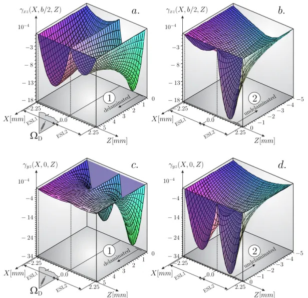
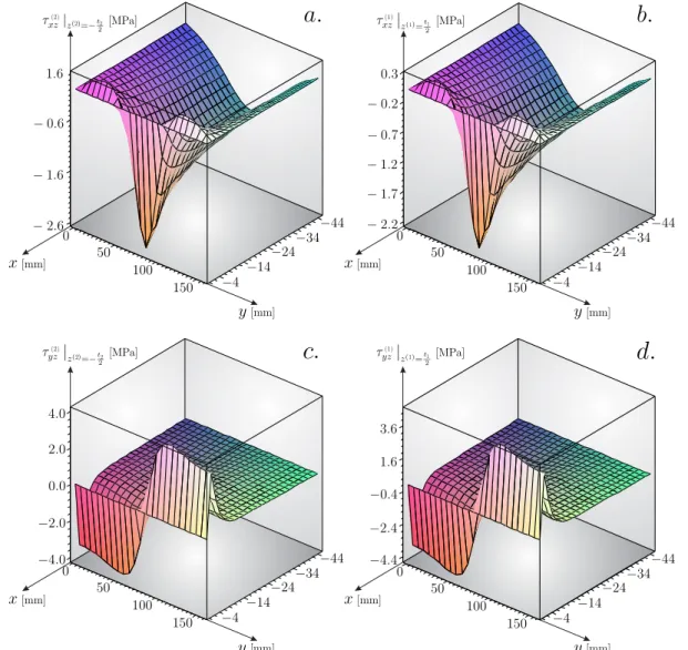
E 3D distributions of shear strains and interlaminar stresses 125

(8)

Nomenclature

Acronyms

AC Autocontinuity

B.C. Boundary condition

C.C. Continuity condition

CFRP Carbon-ﬁbre reinforced plastic CLPT Classical laminated plate theory

ERR Energy release rate

ESL Equivalent single layer

FE Finite element

FEM Finite element method

FSDT First-order shear deformable plate theory GFRP Glass-ﬁbre reinforced plastic

LEFM Linear elastic fracture mechanics ODE Ordinary diﬀerential equation PDE Partial diﬀerential equation

SEKC System of exact kinematic conditions SIF Stress intensity factor

SSCC Shear strain control condition

SSDT Second-order shear deformable plate theory TSDT Third-order shear deformable plate theory VCCT Virtual crack closure technique

Greek Symbols

¯

σ_n(i), ¯τ_ns(i), ¯τ_nz(i) Stresses imposed on the curved edge of the i^th ESL of the plate ψ_(p) Vector of primary parameters

(9)

δσ Virtual stress tensor

δε Virtual strain tensor

Γ_σ(i) Curved edge domain in the plate boundary γ_xz, γ_yz Transverse shear strains

λ Third-order displacement term

ν_xy,ν_xz, ν_yz Poisson’s ratios in the x−y, x−z and y−z planes Ω₀ Surface domain of the plate

Ω_D Plane of delamination

φ Second-order displacement term

ψ_(s)j, ψ_(n)j Vectors of primary parameters in the s, n, z coordinate system ψ_(x)j, ψ_(y)j Vectors of primary parameters in the x, y, z coordinate system

σ_ij Stress tensor

θ Angle of rotation

ε_ij Strain tensor

Roman Symbols

δu, δv, δw Virtual displacement ﬁeld components Δx,Δy,Δz Size of crack tip elements

Lˆ^(x,xy), ˆP^(x,xy) Vectors of equivalent higher-order stress resultants

Mˆ^(x,xy) Vector of equivalent bending and twisting moments

Qˆ_x, ˆQ_y Equivalent transverse shear forces

U Strain energy

W Strain energy density

WF Work of external forces

C^(m)_(i) Stiﬀness matrix

a Delamination length

A_pq Extensional stiﬀness matrix

b Plate width

B_pq Coupling stiﬀness matrix

c Undelaminated length

(10)

NOMENCLATURE

D_pq Bending stiﬀness matrix

E_x, E_y, E_z Moduli of elasticity in the x, y and z directions E_pq, F_pq,G_pq,H_pq Higher-order stiﬀness matrices

G_III Mode-III energy release rate G_II Mode-II energy release rate G_I Mode-I energy release rate G_T Total energy release rate

G_xy,G_xz,G_yz Shear moduli in thex−y,x−z and y−z planes h The number of ESLs in the bottom plate

J_m J-integral,m = 1,2,3 J_III Mode-III J-integral

J_II Mode-II J-integral

k The number of ESLs over the whole thickness K_ij Displacement multiplicator matrix

L_x, L_y, L_xy Higher-order stress resultants M_x, M_y, M_xy Bending and twisting moments

N_l The number of layers in the whole plate N_x, N_y, N_xy In-plane forces

n_x, n_y Components of outward normal on the plate edge N_l(i) The number of layers in the i^th ESL

P_x, P_y, P_xy Higher-order stress resultants

q_b, q_t Surface loads on the bottom and top boundaries Q_x, Q_y Transverse shear forces

R_x, R_y Higher-order shear forces S_x, S_y Higher-order shear forces t_b Thickness of the bottom plate t_i Thickness of thei^th ESL t_t Thickness of the top plate u, v, w Displacement ﬁeld components

X

(11)

u₀,v₀ Global membrane displacements u_0i, v_0i Local membrane displacements

u_0n, u_0s Membrane displacements in the coordinate system of the curved edge of the plate

z⁽ⁱ⁾ Local through the thickness coordinate

z⁽ⁱ⁾_R Coordinate of the global reference plane in the i^th ESL z⁽ⁱ⁾_m, z_m+1⁽ⁱ⁾ Local coordinates of the m^th layer in the i^th ESL

(12)

(13)

Introduction 1

1.1 Application of laminated composite materials in engi- neering structures

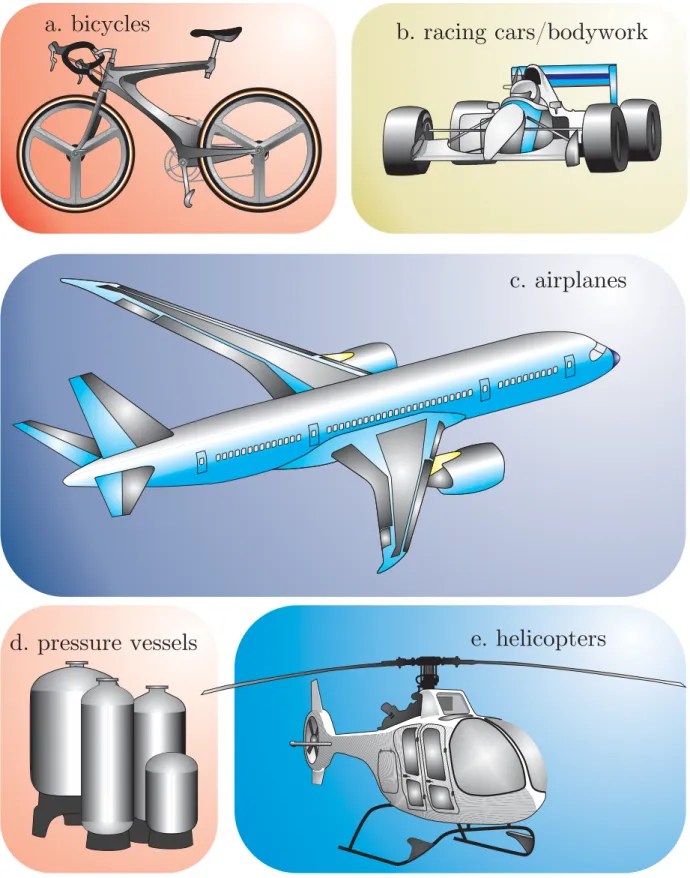
Composites are heterogeneous materials, wherein the high stiffness is provided by the combination of fibres and the matrix material. In many applications the low weight is very important beside the high stiffness and strength. Typical examples are shown in Figures 1.1 and 1.2 discussed briefly in the sequel. The examples were searched and found by using Google.

The ﬁrst example in Figure 1.1 is the bicycle: the frame and even the wheel is made mostly from carbon composites for professional cyclers. The construction in Figure 1.1a enables some elastic deformation for the point of the saddle in contrast with constructions made of metals. The second example is the racing car/bodywork construction (Figure 1.1b).

Formula one cars are constructed by the racing teams themselves by carbon-fibre and other ultra-weight materials. Example 3 in Figure 1.1c is the airplane. The materials used in the Boeing 747 are 50% composites, fiberglass and carbon sandwich materials. Pressure vessels (Figure 1.1d) are manufactured from carbon and glass fiber composites by different technologies. The most important advantage of composite materials over metals in this field is the chemical resistance (Phillips (1989)). Figure 1.1 ends in the helicopters (Figure 1.1e), where lightweight and whisper quiet ride provided by composite materials is very important.

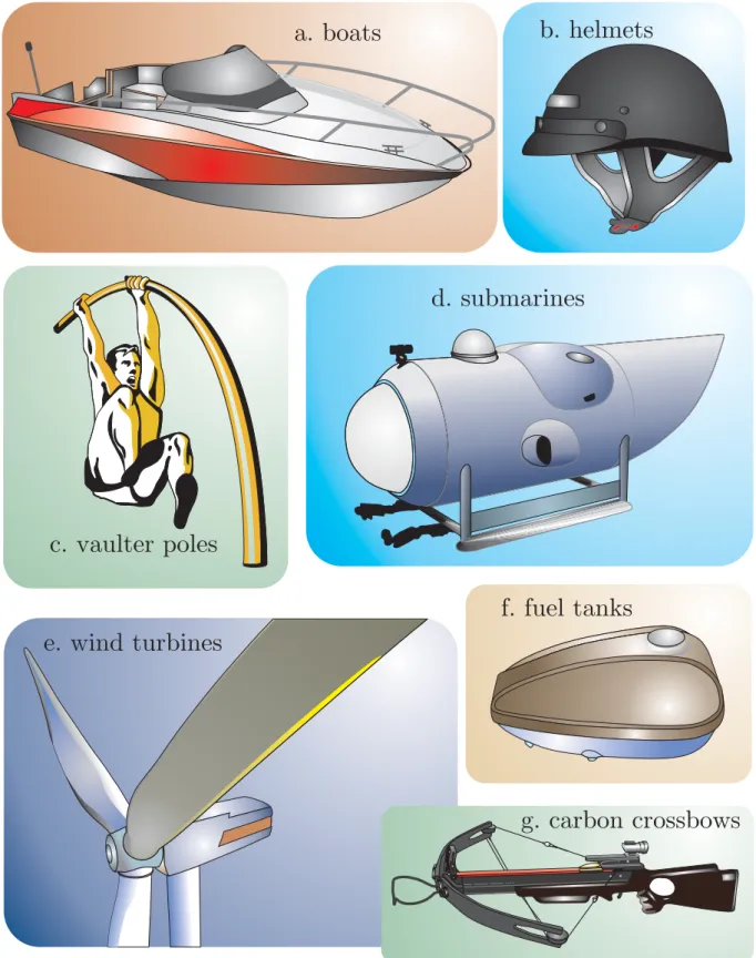
The examples are continued in Figure 1.2 with boats (Figure 1.2a) that are made out of many type of composites. Glass reinforced (polyester and vinylester) plastics have become the most prevalent composites in boatbuilding providing resistance against aggressive marine environment. Helmets (Figure 1.2b) are equally used in sports and military industry. Open and full face helmets are typically manufactured from carbon composites. The excellent shock resistance of composite materials should be highlighted again. Pole vault is one of the most technical of athletic events (Figure 1.2c). The vaulting poles are made out of combination of different materials. The most commonly used are carbon-fibre (CFRP) and glass-fibre reinforced plastics (GFRP). The pole has a diameter of about 50 mm and it is bent to a radius of curvature of about 1 m. The strength of the glass fiber composites is about 2-3 GPa. The key feature in the vaulting pole is the absence of large flaws and the

(14)

CHAPTER 1. INTRODUCTION

a. bicycles

c. airplanes

e. helicopters d. pressure vessels

b. racing cars/bodywork

Figure 1.1: Application examples of composite materials in the engineering life - Part 1.

high toughness providing excellent resistance to fracture. In the field of submarines (Figure 1.2d) the benefits of composite materials - beside resistance against marine environment - are weight reduction, acoustic transparency, damping, thermal insulation and the fact that there is no magnetic signature which makes it very difficult to locate the submarine’s position. The manufacturing technologies of wind turbine blades (Figure 1.2e) has evolved

2

(15)

a. boats

c. vaulter poles

e. wind turbines

g. carbon crossbows f. fuel tanks

b. helmets

d. submarines

Figure 1.2: Application examples of composite materials in the engineering life - Part 2.

over the past twenty years. Lightweight construction is a keyword again in this ﬁeld. The last two examples are: fuel tanks (Figure 1.2f) and carbon crossbows (Figure 1.2g), wherein the lightweight construction and accurate manufacturing is important again.

Beside the many advantages, composite materials are susceptible to various damage modes such as ﬁber breakage, matrix failure, ﬁber pull-out (Adams et al. (2000); Phillips

(16)

(1989)) and among others interlaminar fracture or delamination, which is the main object of this thesis.

1.2 Delamination in composite structures

As it can be seen in Figures 1.1 and 1.2 the basic application area of composite materials is thin- and thick-walled structures, like beams, plates and shells. Delamina- tion fracture in this kind of structures (Kiani et al. (2013); Marat-Mendes and de Freitas (2013); Zhou et al. (2013)) can take place e.g. as the result of low velocity impact (Burlayenko and Sadowski (2012); Christoforou et al. (2008); Ganapathy and Rao (1998);

Goodmiller and TerMaath (2014); Rizov et al. (2005); Wang et al. (2012); Zammit et al.

(2011)), manufacturing defects (Zhang and Fox (2007); Zhou et al. (2013)) and free edge effect (Ahn et al. (2013); Sarvestani and Sarvestani (2012)). The resistance to delamination is characterized by experimental tests under different fracture modes. The main parameters of linear elastic fracture mechanics (LEFM) are the stress intensity factor (SIF) (Anderson (2005); Cherepanov (1997); Hills et al. (1996)) and energy release rate (ERR) (Adams et al. (2000); Anderson (2005)), respectively. The three basic fracture modes are shown in Figure 1.3. The fracture tests are carried out on different type of delamination specimens including mode-I (Hamed et al. (2006); Islam and Kapania (2011); Jumel et al.

(2011a); Kim et al. (2011); Peng et al. (2011); Romhany and Szebenyi (2012); Salem et al.

(2013); Sorensen et al. (2007)), mode-II (Arg¨uelles et al. (2011); Arrese et al. (2010);

Budzik et al. (2013); Jumel et al. (2013); Kutnar et al. (2008); Mladensky and Rizov (2013b); Rizov and Mladensky (2012)), mixed-mode I/II (Bennati et al. (2009, 2013a,b);

Fern´andez et al. (2013); Jumel et al. (2011b); Kenane et al. (2010); Nikbakht and Choupani (2008); da Silva et al. (2011); Szekr´enyes (2007); Yoshihara and Satoh (2009)), mode- III (Johnston et al. (2012); Marat-Mendes and Freitas (2009); Mehrabadi and Khosravan (2013); de Morais and Pereira (2009); de Morais et al. (2011); de Moura et al. (2009);

Pereira et al. (2011); Rizov et al. (2006); Suemasu and Tanikado (2012); Szekr´enyes (2009a)), mixed-mode I/III (Pereira and de Morais (2009); Szekr´enyes (2009b)) mixed- mode II/III (Ho and Tay (2011); Kondo et al. (2011, 2010); Mehrabadi (2013); Miura et al.

(2012); Mladensky and Rizov (2013a); de Morais and Pereira (2008); Nikbakht et al.

(2010); Suemasu et al. (2010); Suemasu and Tanikado (2012); Szekr´enyes (2007);

Szekr´enyes (2012)) and mixed-mode I/II/III (Davidson and Sediles (2011); Davidson et al.

(2010); Szekr´enyes (2011)) tests, respectively. In the former works beam and plate speci- mens were applied. While for beams the closed-form solutions for the ERRs are available, for plates similar solutions exist only for some relatively simple systems including special or in-plane loads (Lee and Tu (1993); Saeedi et al. (2012a,b)).

The plate theories of laminated materials are originated to the classical theories shown in Figure 1.4, which are based on an assumed displacement ﬁeld. The displacement vector ﬁeld is: u =

u v w _T

. In the sequel small displacements and rotations are assumed. The simplest plate theory is the classical laminated plate theory (CLPT) (Koll´ar and Springer (2003); Kumar and Lal (2012); Reddy (2004)), which is based on the Kirchhoﬀ hypothesis:

u(x, y, z) =u₀(x, y)−z∂w

∂x, v(x, y, z) =v₀(x, y)−z∂w

∂y, w(x, y) =w₀(x, y), (1.1) where there are three independent parameters: u₀, v₀ are the membrane displacements and w is the transverse deflection, moreover z is the thickness coordinate. The cross section rotations are approximated by the derivatives of the deflection. The first-order shear

(17)

X

Y Z

X

Y Z

X

Y Mode-I Z

(opening mode)

Mode-II (sliding mode)

Mode-III (tearing mode)

Figure 1.3: Basic fracture modes in linear elastic fracture mechanics.

deformable plate theory (FSDT or Reissner-Mindlin theory) (Ovesy et al. (2015); Reddy (2004); Thai and Choi (2013)) assumes independent rotations (θ_y and θ_x) about the x and y axes:

u(x, y, z) = u₀(x, y)+θ_(x)(x, y)z, v(x, y, z) = v₀(x, y)+θ_(y)(x, y)z, w(x, y, z) =w₀(x, y).

CLPT

¶w¶x

-q^{( )}x

¶w¶x

¶w¶x x u, z

z w,

x

-q^{( )}^x

-q^{( )}^x u⁰

( , )u w

( , )u w FSDT

SSDT

TSDT

z

x

y

Figure 1.4: The deformation of a material line of a laminated plate on the x−z plane in accordance with the diﬀerent plate theories.

(18)

(1.2) The higher-order plate theories can be obtained by the generalization of the FSDT displacement ﬁeld even in the thickness direction:

u(x, y, z) =u₀(x, y) +θ_(x)(x, y)z+φ_(x)(x, y)z²+λ_(x)(x, y)z³+. . . , v(x, y, z) =v₀(x, y) +θ_(y)(x, y)z+φ_(y)(x, y)z² +λ_(y)(x, y)z³+. . . , w(x, y, z) =w₀(x, y) +θ_(z)(x, y)z+φ_(z)(x, y)z²+λ_(z)(x, y)z³ +. . . ,

(1.3)

where θ_(m) means the angle of rotation (or first-order term), φ_(m) is the second-order, λ_(m) (m = x, y, z) is the third-order displacement term. Moreover, the second-order shear de- formable plate theory (SSDT) (Izadi and Tahani (2010);Szekr´enyes (2013b, 2015)) is ob- tained if we consider the terms in the displacement field upto z², a general third-order plate theory (TSDT) means that each component is approximated by a cubic function (Panda and Singh (2011); Singh and Panda (2014);Szekr´enyes (2014d)). If even the normal deformation is taken into account then the approach means a shear and normal deformable theory (Sahoo et al. (2016)). Among these approaches the Reddy third-order shear deformable theory should be mentioned (Reddy (2004)). This theory satisfies the dynamic boundary condition at the top and bottom plate surfaces (traction-free surfaces). The orig- inal idea is related to the name of Levinson (1980), who applied the concept to isotropic materials. Later, Reddy extended this theory to laminated composites. The displacement field of Reddy TSDT takes the form of:

u(x, y, z) =u₀(x, y) +θ_(x)(x, y)z− 4 3t²

θ_(x)+∂w₀

∂x

z³, v(x, y, z) =v₀(x, y) +θ_(y)(x, y)z− 4

3t²

θ_(y)+∂w₀

∂y

z³, w(x, y) =w₀(x, y),

(1.4)

wheret is the plate thickness and it is conspicuous that the second-order terms are missing.

These are the so-called equivalent single-layer theories (ESL), in which a heterogeneous laminated plate is treated as a statically equivalent single layer having a complex constitutive behavior Reddy (2004). Within an ESL the displacement ﬁeld is approximated by a given set of functions. An important aspect of these approaches is that if the normal deformability is not taken into account, then plane stress condition is assumed, therefore the transverse normal stress σ_z does not appear in the equations. The literature also oﬀers the 3D elasticity solution and the layerwise or multilayer approaches (Batista (2012); Ferreira et al.

(2011); Reddy (2004); Saeedi et al. (2012a,b)) (3D solutions), which can further improve the accuracy of the solution. In the book of Reddy (2004) and Kollár and Springer (2003) the application of the ESL theories to perfect plates (no imperfections and material defects) is well-documented and many examples are presented. It is important to note that Reddy (2004) concluded that the contribution of the higher-order theories to the solution of the plate bending problems compared to the CLPT and FSDT is not meaningful, however these are computationally significantly more expensive and sometimes it is absolutely sufficient to apply the CLPT or FSDT.

This paper puts emphasis essentially on the application of plate theories in fracture mechanics under mixed-mode II/III condition. In this respect the work by Davidson et al.

(2000) is noteworthy, wherein the ERRs in delaminated plates were calculated by using

(19)

Mindlin-type plate finite elements (FSDT). The results were compared to 3D FE calculations, but the agreement was not satisfactory in all cases. One of the reasons for that could be the lack of higher-order plate finite elements in the commercial FE packages. A similar work was published by (Sankar and Sonik (1995)), as well. Some late works investigated the same problem (Bruno et al. (2003, 2005)) with the aid of interface and contact elements providing accurate results, however, the formulation was quite complicated and difficult to implement in commercial FE packages. Other formulations are available in the field, however, each is based on the FSDT and the virtual crack closure concept (Qing et al. (2011); Zou et al.

(2001)).

1.3 Main aims and analysis methods

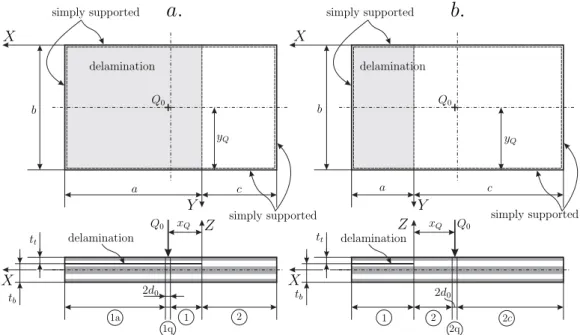
In delaminated plates and shells the presence of the delamination tips means a perturbation in the mechanical ﬁelds and a more accurate description could be necessary for a fracture mechanical analysis than those provided by CLPT and FSDT. The main aim of this thesis is to solve the most essential plate bending problems in that case when the plate contains a through-width delamination using higher-order plate theories. To the best of the author’s knowledge these examples are not yet documented in the literature. A successful assessment of plate theories can be the basis for the development of plate and shell ﬁnite elements for the modeling of delaminations.

This thesis is organized as follows. In Chapter 2 the basic equations of laminated third- order plates is presented. This chapter is based on the system of exact kinematic conditions.

A modified third-order displacement field and the displacement multiplicator matrix is developed and the principle of virtual work is utilized to derive the equilibrium equations of delaminated plates. The formulation is valid for laminated composite plates made out of any materials (e.g. polymer matrix composite) that behave as linear elastic material. Chapter 3 describes the method of 2ESLs and the general equations are derived for FSDT, SSDT and Reddy TSDT. It has to be mentioned that the CLPT was found to be inappropriate to capture the problems discussed in this thesis with an acceptable accuracy (Szekr´enyes (2012, 2013a, 2014a)). An important part of Chapter 3 is the introduction of the equivalent stress resultants. Chapter 4 contains the details of the method of 4ESLs, wherein four subplates are applied over the thickness of the plate. In this chapter the FSDT, SSDT and TSDT equations are given. In Chapter 5 two examples are solved by using the Lévy plate formulation. The state-space model of the plate system is derived separately for the undelaminated and delaminated regions, respectively. At the same time the generalized continuity conditions are given by parameter sets, even the boundary conditions are described for simply supported, built-in and free edges. Chapter 6 presents the results for the displacement and stress fields and a comparison is made to 3D FE results. In Chapter 7 the 3D J-integral is applied using the higher-order plate theories and analytical expressions are developed for the calculation of the mode-II and mode-III energy release rates. In the same chapter the distribution of the J-integrals along the delamination front of delaminated composite plates is presented and compared to the result of the 3D FE analysis. The methods of 2ESLs and 4ESLs are also compared to each other and the ranking of the different theories is made.

Chapter 8 summarizes the main results and presents the novel scientiﬁc results in the form of theses. Finally, the possible application areas of the results are brieﬂy given.

(20)

The basic equations of delaminated composite 2

plates

top plate top plate

bottom plate bottom plate

top plate

bottom plate

Figure 2.1: Plate elements with orthotropic plies and the position of the delamination over the plate thickness, cases I, II, III and IV.

In this chapter the basic equations of delaminated plates are presented. The formulation is based on the semi-layerwise modeling technique. The concept is shown in Figure 2.1 indicating plate elements with an interfacial delamination. The delamination divides the plate into a top and a bottom subplate. The top and the bottom subplates are further divided into equivalent single layers. In Figure 2.1 the method of 4ESLs is presented, i.e.

the top and bottom plates are captured by two ESLs (altogether 4ESLs are applied).

(21)

Definition:semi-layerwise plate model. If a laminated plate with N_l number of layers is modeled byN_ESL number of equivalent single layers andN_ESL < N_l then the model is called semi-layerwise plate model. In this case the stiﬀness parameters and matrices of each ESL has to be determined with respect to the local reference planes of the ESLs. The interface planes between the neighboring ESLs are the perturbation planes. If N_ESL = N_l then the model is a standard layerwise model.

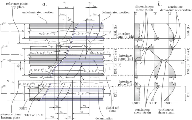
Figure 2.2: Cross sections and deformation of the top and bottom plate elements of a delaminated plate in the X-Z plane (a). Distribution of the transverse shear strains by FSDT, SSDT and TSDT (b).

Figure 2.2 shows the section of the transition between the delaminated and undelaminated regions of the layered plate element in theX−Z plane, while in Figure 2.3 the Y −Z plane is shown. The two coordinate systems are to show the displacement parameters in the undelaminated and delaminated parts. The elements contain an interfacial delamination (delaminated portion) parallel to the Y axis, i.e. it goes across the entire plate width (refer to Figure 2.1). The general case involves k number of ESLs applied through the whole thickness. The transverse splitting means that the undelaminated and delaminated regions are captured by different mathematical models. In accordance with the literature review the ESLs can be captured by different plate theories. In this chapter we apply the FSDT, SSDT and TSDT theories. The general third-order Taylor series expansion of the in-plane displacement functions results in the following displacement field (Panda and Singh (2009, 2011); Singh and Panda (2014); Talha and Singh (2010)):

u_(i)(x, y, z⁽ⁱ⁾) =u₀(x, y) +u_0i(x, y) +θ_(x)i(x, y)z⁽ⁱ⁾+φ_(x)i(x, y)[z⁽ⁱ⁾]²+λ_(x)i(x, y)[z⁽ⁱ⁾]³, v_(i)(x, y, z⁽ⁱ⁾) =v₀(x, y) +v_0i(x, y) +θ_(y)i(x, y)z⁽ⁱ⁾+φ_(y)i(x, y)[z⁽ⁱ⁾]²+λ_(y)i(x, y)[z⁽ⁱ⁾]³, w_(i)(x, y) =w(x, y),

(2.1)

(22)

PLATES

Figure 2.3: Cross sections and deformation of the top and bottom plate elements of a delaminated plate in the Y-Z plane (a). Distribution of the transverse shear strains by FSDT, SSDT and TSDT (b).

whereiis the index of the actual ESL,z⁽ⁱ⁾ is the local through thickness coordinate of thei^th ESL and always coincides with the local midplane,u₀andv₀are the global,u_0iandv_0i are the local membrane displacements, moreover, θ means the rotations of the cross sections about the X and Y axes (refer to Figure 2.1),φ denotes the second-order,λ represents the third- order terms in the displacement functions. Finally w_(i) is the transverse deﬂection function.

Eq.(2.1) will be applied equally to the undelaminated and delaminated portions and the continuity between these parts will be established. In this thesis only shear deformable plate models are developed, in other words the deﬂection is inextensible in the through-thickness direction involving thatw_(i)(x, y) =w(x, y). The displacement functions of FSDT and SSDT can be obtained by reducing Eq.(2.1) and taking φ_(x)i = φ_(y)i = 0 and λ_(x)i = λ_(y)i = 0, respectively (Izadi and Tahani (2010); Petrolito (2014)). The displacement ﬁeld given by Eq.(2.1) is associated to each ESL.

2.1 The system of exact kinematic conditions

The displacement vector ﬁeld for the i^th ESL is u_(i) =

u_(i) v_(i) w_(i) _T

. The kinematic continuity between the displacement fields of adjacent ESLs is established by the system of exact kinematic conditions (SEKC), which was originally developed by Szekrényes (2013c, 2014c, 2015, 2016a,b). The first set of conditions formulates the continuity of the in-plane and transverse displacements between the neighboring plies as (refer to Figures 2.2 and 2.3):

(u_(i), v_(i), w_(i))

z⁽ⁱ⁾=ti/2 = (u_(i+1), v_(i+1), w_(i+1))

z⁽ⁱ⁺¹⁾=−ti+1/2, (2.2)

where t_i is the thickness of the speciﬁed layer. It has to be noted that the result of Eq.(2.2) was applied by Davidson et al. (2000) and Zou et al. (2001), however their equations are

(23)

valid only for the FSDT. On the contrary, Eq.(2.2) is more general and applicable to any plate theory. Moreover, there are large number of works referred to in the book of Reddy (2004)applying displacement continuity between the layers. Those works apply full layerwise models to perfect plates, in contrast with this thesis, which deals with the semi-layerwise analysis of delaminated plates. The second set of conditions deﬁnes the global membrane displacements (u₀, v₀) at the reference plane of the actual region. If the coordinate of the global reference plane is z_R⁽ⁱ⁾ and is located in the i^th layer, then the conditions become:

u_(i)

z⁽ⁱ⁾=z⁽ⁱ⁾_R −u₀ = 0, v_(i)

z⁽ⁱ⁾=z⁽ⁱ⁾_R −v₀ = 0. (2.3)

The two sets of conditions given by Eqs.(2.2)-(2.3) are suﬃcient to develop semi-layerwise models using the FSDT. If the SSDT or TSDT is applied, then we can impose the shear strain continuity at the interface (or perturbation) planes. In accordance with Figures 2.2b and 2.3b these conditions are formulated as:

(γ_xz(i), γ_yz(i))

z⁽ⁱ⁾=ti/2 = (γ_xz(i+1), γ_yz(i+1))

z⁽ⁱ⁺¹⁾=−ti+1/2. (2.4)

It has to be mentioned that in general layerwise models assume continuous shear stresses at the interfaces (Reddy (2004)). For the TSDT theory two more sets of conditions are reasonable to introduce. The imposition of continuity of the ﬁrst and second derivatives of the shear strain (Szekr´enyes (2016b)) prevents the unwanted oscillations (and the too large compliance) in the shear stress distributions (see Figures 2.2b and 2.3b):

∂γ_xz(i)

∂z⁽ⁱ⁾ ,∂γ_yz(i)

∂z⁽ⁱ⁾

z⁽ⁱ⁾=ti/2

=

∂γ_xz(i+1)

∂z⁽ⁱ⁺¹⁾ ,∂γ_yz(i+1)

∂z⁽ⁱ⁺¹⁾

z⁽ⁱ⁺¹⁾=−ti+1/2

, (2.5)

and:

∂²γ_xz(i)

∂(z⁽ⁱ⁾)²,∂²γ_yz(i)

∂(z⁽ⁱ⁾)²

z⁽ⁱ⁾=ti/2

=

∂²γ_xz(i+1)

∂(z⁽ⁱ⁺¹⁾)²,∂²γ_yz(i+1)

∂(z⁽ⁱ⁺¹⁾)²

z⁽ⁱ⁺¹⁾=−ti+1/2

. (2.6)

An important addition to Eqs.(2.2)-(2.6) is the so-called shear strain control condition (SSCC, Szekr´enyes (2016a)). The set of conditions applied is:

(γ_xz(l), γ_yz(l))

z^(l)=−tl/2 = (γ_xz(m), γ_yz(m))

z^(m)=tm/2, (2.7)

wherelandmdenote ESLs at the boundaries, where the shear strains are equal to each other and m > l always. In accordance with Reddy theory (Reddy (2004)) the top and bottom surfaces of the plate are traction-free (zero shear stresses). If the system is modeled by 4ESLs the traction-free conditions leads to overconstraining (or stiﬀening) of the model and wrong results are obtained. Therefore, instead of imposing zero stresses at the free surfaces we impose the identical shear strain values at the boundary planes by Eq.(2.7). Essentially, the SSCC is applicable only if at least 4ELSs and the SDDT or TSDT are applied.

Based on the linear elasticity and assuming transversely inextensible deﬂection in each ESL, the SEKC formulates conditions using the in-plane displacement functions:

∂ⁿ(u_(i),v_(i))

∂(z⁽ⁱ⁾)ⁿ , n = 0,1,2,3, where n = 0 means condition against in-plane displacement, n = 1 means condition for shear strain, if n = 2 and n = 3 then a condition for the shear strain’s ﬁrst and second derivative is formulated. The SEKC conditions can be applied equally to the undelaminated and delaminated portions of the plate. Moreover these conditions can be implemented into any plate theory.

(24)

PLATES

2.2 Kinematically admissible displacement fields

In Eq.(2.1) the displacement functions are modiﬁed in order to satisfy Eqs.(2.2)-(2.7). In the general sense, by applying the FSDT, SSDT and TSDT theories the in-pane displacement functions can be written as:

u_(i) =u₀+

K_ij⁽⁰⁾+K_ij⁽¹⁾z⁽ⁱ⁾+K_ij⁽²⁾[z⁽ⁱ⁾]²+K_ij⁽³⁾[z⁽ⁱ⁾]³

ψ_(x)j, i= 1..k, v_(i)=v₀ +

K_ij⁽⁰⁾+K_ij⁽¹⁾z⁽ⁱ⁾+K_ij⁽²⁾[z⁽ⁱ⁾]² +K_ij⁽³⁾[z⁽ⁱ⁾]³

ψ_(y)j, i= 1..k,

(2.8) where K_ij is the displacement multiplicator matrix and related exclusively to the geometry (ESL thicknesses), irefers to the ESL number, the summation indexjdeﬁnes the component inψ, which is the vector of primary parameters (see later), ﬁnallyw_(i)(x, y) =w(x, y) for each ESLs, i.e. the transverse normal of each ESL is inextensible (Reddy (2004)). Eq.(2.8) can be obtained by parameter elimination. It is important to note that the size and the elements of ψ depend on the applied theory, the number of ESLs and the number of conditions applied.

Definition: Parameter elimination, primary and secondary parameters. Certain param- eters of the in-plane displacement functions can be eliminated using the SEKC requirements.

The remaining (orprimary) parameters are untouched, the parameters to be eliminated are the secondary parameters. The local membrane displacements are typically secondary parameters, the global membrane displacements are primary parameters, the rotations, second- and third-order parameters are mixed (either primary or secondary) parameters.

In the subsequent sections the undelaminated and delaminated regions are discussed separately. First, the TSDT is considered and the SSDT and FSDT ﬁeld equations are obtained by the reduction of TSDT model.

2.3 Virtual work principle and constitutive equations

The strain ﬁeld in an elastic body in terms of the displacement ﬁeld is obtained by the following equation (assuming small displacements and strains) (Chou and Pagano (1967)):

ε_pq = 1

2(u_p,q+u_q,p), p, q= 1,2 or 3, (2.9)

where ε_pq is the strain tensor, u_p is the displacement vector ﬁeld and the comma means diﬀerentiation with respect to the index right after. By assuming plane stress state (σ_z(i)= 0) in the plate and using Eqs.(2.1)-(2.9) the vector of in-plane strains becomes (Reddy (2004)):

⎛

⎝ ε_x ε_y γ_xy

⎞

⎠

(i)

=

⎛

⎜⎝ ε⁽⁰⁾_x ε⁽⁰⁾_y γ_xy⁽⁰⁾

⎞

⎟⎠

(i)

+z⁽ⁱ⁾·

⎛

⎜⎝ ε⁽¹⁾_x ε⁽¹⁾_y γ_xy⁽¹⁾

⎞

⎟⎠

(i)

+ z⁽ⁱ⁾2

·

⎛

⎜⎝ ε⁽²⁾_x ε⁽²⁾_y γ_xy⁽²⁾

⎞

⎟⎠

(i)

+ z⁽ⁱ⁾3

·

⎛

⎜⎝ ε⁽³⁾_x ε⁽³⁾_y γ_xy⁽³⁾

⎞

⎟⎠

(i)

, (2.10)

or{ε}_(i) = ε⁽⁰⁾

(i)+z⁽ⁱ⁾· ε⁽¹⁾

(i)+ z⁽ⁱ⁾₂

· ε⁽²⁾

(i)+ z⁽ⁱ⁾₃

· ε⁽³⁾

(i) which is third-order in terms of the through-thickness coordinate,z⁽ⁱ⁾. The vector of transverse shear strains is:

γ_xz γ_yz

(i)

=

γ_xz⁽⁰⁾ γ_yz⁽⁰⁾

(i)

+z⁽ⁱ⁾·

γ_xz⁽¹⁾ γ_yz⁽¹⁾

(i)

+ z⁽ⁱ⁾₂

·

γ_xz⁽²⁾ γ_yz⁽²⁾

(i)

, (2.11)

(25)

or in a compact form: {γ}_(i) = γ⁽⁰⁾

(i)+z⁽ⁱ⁾· γ⁽¹⁾

(i)+ z⁽ⁱ⁾₂

· γ⁽²⁾

(i), which is second- order in terms of z⁽ⁱ⁾. To derive the governing equations of the plate system we apply the virtual work principle (Reddy (2004)):

T1

T0

(δU −δW_F)dt= 0, δU =

i

δU_(i), δW_F =

i

δW_F_(i), (2.12)

whereU is the strain energy, W_F is the work of external forces andtis the time (L=U −W_F is the Lagrange function). The virtual strain energy for the i^th ESL of the plate system including the delaminated and undelaminated regions is (Reddy (2004)):

δU(i) =

V

σ(i):δε(i)dV =

Ω0

⎧⎪

⎨

⎪⎩

ti/2

−ti/2

σ_x(i)δε_x(i)+σ_y(i)δε_y(i)+τ_xy(i)δγ_xy(i)+τ_xz(i)δγ_xz(i)+τ_yz(i)δγ_yz(i) dz⁽ⁱ⁾

⎫⎪

⎬

⎪⎭dxdy, (2.13) whereσ(i) is the stress tensor, δε(i) is the virtual strain tensor of thei^thESL, Ω₀ denotes the surface domain of the plate in the global X−Y (or x−y) plane. The double dot product means: σ(i) :δε(i) =σ_ij(i)δε_ij(i). The virtual work of the external forces for a single ESL is:

δWF(i) =

Ω0

q_b(i)(x, y)δw(x, y,−t_i/2) +q_t(i)(x, y)δw(x, y, t_i/2) dxdy

+

Γσ(i)

⎧⎪

⎨

⎪⎩

ti/2

−ti/2

σ¯_n(i)δu_n(i)+ ¯τ_ns(i)δu_s(i)+ ¯τ_nz(i)δw_(i) dz⁽ⁱ⁾

⎫⎪

⎬

⎪⎭ds,

(2.14)

whereq_b andq_tare the surface loads on the top and bottom plane of thei^th ESL. The second term in the expression above is related to the virtual work of the imposed stress components (¯σ_n(i), ¯τ_ns(i) and ¯τ_nz(i)) acting on the curved edge boundary denoted by Γ_σ(i), moreover s and n are the tangential and normal directions (Reddy (2004)). Taking back the strain ﬁeld (Eqs.(2.10)-(2.11)) into Eq.(2.13) we obtain:

δU_(i) =

Ω0

⎧⎪

⎨

⎪⎩

ti/2

−ti/2

σ_x(i)

δε⁽⁰⁾_x(i)+z⁽ⁱ⁾δε⁽¹⁾_x(i)+ (z⁽ⁱ⁾)²δε⁽²⁾_x(i)+ (z⁽ⁱ⁾)³δε⁽³⁾_x(i)

+σ_y(i)

δε⁽⁰⁾_y(i)+z⁽ⁱ⁾δε⁽¹⁾_y(i)+ (z⁽ⁱ⁾)²δε⁽²⁾_y(i)+ (z⁽ⁱ⁾)³δε⁽³⁾_y(i)

+τ_xy(i)

δγ_xy(i)⁽⁰⁾ +z⁽ⁱ⁾δγ⁽¹⁾_xy(i)+ (z⁽ⁱ⁾)²δγ_xy(i)⁽²⁾ + (z⁽ⁱ⁾)³δγ_xy(i)⁽³⁾

+τ_xz(i)

δγ_xz(i)⁽⁰⁾ +z⁽ⁱ⁾δγ_xz(i)⁽¹⁾ + (z⁽ⁱ⁾)²δγ_xz(i)⁽²⁾

+τ_yz(i)

δγ_yz(i)⁽⁰⁾ +z⁽ⁱ⁾δγ_yz(i)⁽¹⁾ + (z⁽ⁱ⁾)²δγ_yz(i)⁽²⁾

dz⁽ⁱ⁾ dxdy.

(2.15)

(26)

PLATES

The third-order displacement ﬁeld component in Eq.(2.8) can be written as: u_p(i) = u⁽⁰⁾_p(i)+ z⁽ⁱ⁾u⁽¹⁾_p(i)+ [z⁽ⁱ⁾]²u⁽²⁾_p(i)+ [z⁽ⁱ⁾]³u⁽³⁾_p(i), where p=s orn. Taking its virtual form, the virtual work of external forces becomes:

δWF(i) =

Ω0

q_b(i)(x, y)δw(x, y,−t_i/2) +q_t(i)(x, y)δw(x, y, t_i/2) dxdy

+

Γ_σ(i)

⎧⎪

⎨

⎪⎩

ti/2

−ti/2

σ_n(i)

δu⁽⁰⁾_n(i)+z⁽ⁱ⁾δu⁽¹⁾_n(i)+ (z⁽ⁱ⁾)²δu⁽²⁾_n(i)+ (z⁽ⁱ⁾)³δu⁽³⁾_n(i)

+τ_ns(i)

δu⁽⁰⁾_s(i)+z⁽ⁱ⁾δu⁽¹⁾_s(i)+ (z⁽ⁱ⁾)²δu⁽²⁾_s(i)+ (z⁽ⁱ⁾)³δu⁽³⁾_s(i)

+ τ_nz(i)δw_(i)

dz⁽ⁱ⁾ ds.

(2.16) To derive δU(i) and δWF(i) in terms of the stress resultants and the virtual displacement parameters of the plate system we use the constitutive equation. The constitutive equation for orthotropic materials under plane stress state is σ^(m)_(i) =C^(m)_(i) ε^(m) (Koll´ar and Springer (2003); Reddy (2004)), which expands to:

⎛

⎜⎜

⎝ σ_x σ_y τ_yz τ_xz τ_xy

⎞

⎟⎟

⎠

(m)

(i)

=

⎛

⎜⎜

⎝

C₁₁ C₁₂ 0 0 0 C₁₂ C₂₂ 0 0 0

0 0 C₄₄ 0 0

0 0 0 C₅₅ 0

0 0 0 0 C₆₆

⎞

⎟⎟

⎠

(m)

(i)

⎛

⎜⎜

⎝ ε_x ε_y γ_yz γ_xz γ_xy

⎞

⎟⎟

⎠

(i)

, (2.17)

where C^(m)_(i) is the stiﬀness matrix of the m^th layer within the i^th ESL. By using the constitutive equations the stress resultants are calculated by integrating the stresses over the thicknesses of each ESL:

⎛

⎜⎜

⎝ N_αβ M_αβ L_αβ P_αβ

⎞

⎟⎟

⎠

(i)

=

ti/2

−ti/2

σ_αβ

⎛

⎜⎜

⎝ 1 z z² z³

⎞

⎟⎟

⎠

(i)

dz⁽ⁱ⁾,

⎛

⎝ Q_α R_α S_α

⎞

⎠

(i)

=

ti/2

−ti/2

τ_αz

⎛

⎝ 1 z z²

⎞

⎠

(i)

dz⁽ⁱ⁾, (2.18)

whereαandβtakesxory. The relationship between the strain ﬁeld and the stress resultants can be determined by taking back Eqs.(2.17) and (2.10)-(2.11) resulting in the following:

(Szekr´enyes (2014c)):

⎛

⎜⎜

⎝ { N} {M} { L} { P}

⎞

⎟⎟

⎠

(i)

=

⎡

⎢⎢

⎣

[A] [B] [D] [E]

[B] [D] [E] [F] [D] [E] [F] [G]

[E] [F] [G] [H]

⎤

⎥⎥

⎦

(i)

⎛

⎜⎜

⎝

{ε⁽⁰⁾} {ε⁽¹⁾} {ε⁽²⁾} {ε⁽³⁾}

⎞

⎟⎟

⎠

(i)

, (2.19)

⎛

⎝ {Q} {R} {S}

⎞

⎠

(i)

=

⎡

⎣ [A] [B] [D]

[B] [D] [E]

[D] [E] [F]

⎤

⎦

(i)

⎛

⎝ { γ⁽⁰⁾} { γ⁽¹⁾} { γ⁽²⁾}

⎞

⎠

(i)

, (2.20)

Nonsingular delamination modeling in orthotropic composite plates by semi-layerwise analysis