Elastic Analysis of Heterogeneous Thick Cylinders Subjected to Internal or External Pressure Using Shear Deformation Theory

(1)

Elastic Analysis of Heterogeneous Thick Cylinders Subjected to Internal or External Pressure Using Shear Deformation Theory

Mehdi Ghannad

Mechanical Engineering Faculty, Shahrood University of Technology, University Boulevard, Haft Tir Square, Shahrood, Iran

email: mghannadk@shahroodut.ac.ir

Mohammad Zamani Nejad

Mechanical Engineering Department, Yasouj University, Daneshjo Street, P. O.

Box: 75914-353, Yasouj, Iran email: m_zamani@yu.ac.ir

Abstract: An analytical formulation based on the first-order shear deformation theory (FSDT) is presented for axisymmetric thick-walled heterogeneous cylinders under internal and external uniform pressure. It is assumed that the material is isotropic heterogeneous with constant Poisson's ratio and radially varying elastic modulus. First, general governing equations of the heterogeneous thick cylinders are derived by virtual work principle, and using FSDT. Then the obtained equations are solved under the generalized plane strain assumptions. The results are compared with the findings of both plane elasticity theory (PET) and finite element method (FEM).

Keywords: thick cylinder; shear deformation theory (SDT); heterogeneous; functionally graded material (FGM); finite element method (FEM)

1 Introduction

Axisymmetric hollow shells are important in industries. In order to optimize the weight, displacement and stress distribution of a shell, one approach is to use shells with Functionally Graded Materials. FGMs or heterogeneous materials are advanced composite materials with microscopically inhomogeneous character that are engineered to have a smooth spatial variation of continuous properties. The concept of FGMs was proposed by material scientists in Japan [1].

(2)

1.1 Homogeneous Cylinders

First Lamé (1852) found the stress distribution in an isotropic homogeneous hollow cylinder under uniform pressure.This solution has been extensively used to solve many engineering problems. Naghdi and Cooper [2] started with a Reissner's variational theorem and included the effects of shear deformation. The first order displacement field for thick cylindrical shells was expressed by Mirsky- Hermann [3] which is the extension of the Mindlin plate theory [4] and includes transverses shear deformation. Greenspon [5] compared the results of different theories of thick-walled cylindrical shells. Ziv and Perl [6] obtained the response of vibration analysis of a thick-walled cylindrical shell using FSDT theory and solved by finite difference method. Suzuki et al. [7] used the FSDT for vibration analysis of axisymmetric cylindrical shell with variable thickness. They assumed that the problem is in the state of plane stress and ignored the normal stress in the radial direction. Simkins [8] used the FSDT for determining displacement in a long and thick tube subjected to moving loads. Eipakchi et al. [9] used the FSDT for driving governing equations of thick cylinders with varying thickness and solved the equations with perturbation theory. Using FSDT, Ghannad and Zamani Nejad [10] present the general method for analysis of internally pressurized thick- walled cylindrical shells with clamped-clamped ends.

1.2 Heterogeneous Cylinders

Heterogeneous composite materials are functionally graded materials (FGMs) with gradient compositional variation of the constituents from one surface of the material to the other which results in continuously varying material properties.

These materials are advanced, heat resisting, erosion and corrosion resistant, and have high fracture toughness. The FGMs concept is applicable to many industrial fields such as aerospace, nuclear energy, chemical plants, electronics, biomaterials, and so on. Fukui and Yamanaka [11] used the PET for the derivation of the governing equation of a thick-walled FGM tube under internal pressure and solved the obtained equation numerically by means of the Runge-Kutta method.

Horgan and Chan [12] analyzed a pressurized hollow cylinder in the state of plane strain. The exact solution for stresses in FGM pressure vessels alone using Lamé's solution was provided by Tutuncu and Ozturk [13]. They assumed material stiffness obeys a simple power law through the wall thickness with Poisson's ratio being constant. In this reference formula and plot for circumferential stress are incorrect. Jabbari et al. [8] have presented a general analysis of one-dimensional steady-state thermal stresses in a hollow thick cylinder made of FGM. Hongjun et al. [14] and Zhifei et al. [15] provided elastic analysis and an exact solution for stresses in FGM hollow cylinders in the state of plane strain with isotropic multi- layers based on Lamé's solution. Thick-walled cylinders with exponentially- varying material properties were solved by Tutuncu [16]. Zamani Nejad et al. [17]

(3)

developed 3-D set of field equations of FGM thick shells of revolution in curvilinear coordinate system by tensor calculus. Ghannad et al. [18] provided a general axisymmetric solution of FGM cylinders based on PET in the state of plane stress, plane strain and closed cylinder. Abedi et al. [19] obtained a numerical solution using finite element method and a static analysis for stresses and displacements in FGM parabolic solid cylinder.

The following topics will be described; using FSDT, PET and FEM, the heterogeneous hollow cylinders have been solved and have been compared with homogenous cylinders.

2 Governing Equations

In the Plane Elasticity Theory (PET), axisymmetric thick cylinders with constant thickness and uniform pressure are analyzed by Lamé's solution in cylindrical coordinates. The radial displacement of this cylinder is given by:

2 1 r

u C r C

= + r (1) where C₁ and C₂ are constants and r is the radius of cylinder. Consider FGM circular cylindrical shell shown in Fig. 1.

In this figure, P_i and P_o are internal and external pressures, R is the radius of the middle surface and z is the distance from the middle surface which ranges in such an interval as

(

^-^h ²^{≤ ≤}^z ^h ²

)

, so one can write:

2

1( )

r

r R z u C R z C

R z

= + ⇒ = + +

+

(2) If z R <1 and by Taylor expansion:

2 3

2

1( ) 1 2 3

r

C z z z

u C R z

R R R R

⎛ ⎞

= + + ⎜⎝ − + − +"⎟⎠

2 2

1 1 2 3

C C C

z z

C R C

R R R

⎛ ⎞ ⎛ ⎞

=⎜⎝ + ⎟ ⎜⎠ ⎝+ − ⎟⎠ + +"

(3)

The radial displacement is:

2

0 1 2

ur =u +u z+u z +"

(4)

This means that the displacement can be written as a polynomial of z, and u₀ is the displacement of the middle surface (if z=0). h and L are the thickness and the length of the cylinder, in which r_i and r_oare inner and outer radiuses of the cylinder.

The general axisymmetric displacement field in FSDT can be expressed on the basis of axial displacement and radial displacement, as follows:

( ) ( ) , 0 , ( ) ( )

x z

U =u x +φ x z U_θ = U =w x +ψ x z

(5) where u x( )and w x( )are the displacement components of the middle surface.

Also, φ( )x and ψ( )x are the functions used to determine the displacement field.

The strain-displacement relations in the cylindrical coordinates system are:

x z

x

z z

z xz

U du d U w

z z

x dx dx r R z R z

U

U U dw d

z z x dx dx z

θ

φ ψ

ε ε

ε ψ γ φ ψ

⎧ =∂ = + = = +

⎪ ∂ + +

⎪⎨ ∂ ∂ ∂ ⎛ ⎞

⎪ = = = + =⎜ + ⎟+

⎪ ∂ ∂ ∂ ⎝ ⎠

⎩

(6)

Figure 1 Geometry of the cylinder

The elastic modulus is assumed to vary as follows:

( )

n n

i i

i

E r E r E r r

= = ⎛ ⎞⎜ ⎟

⎝ ⎠

(7) By substituting r= +R z into Eq. (7), ^{E z}

( )

is defined as:

( )

( ) +

n i n

i n

i i

R z E

E z E R z

r r

⎛ + ⎞

= ⎜ ⎟ =

⎝ ⎠

(8)

(5)

Here, E_i is Young's modulus of the inner surface and n is inhomogeneity constant. In the present paper n is assumed to range − ≤ ≤2 n 2. Further, the Poisson's ratio υ is assumed a constant. Therefore, the stress-strain relations are:

( ) 1 (1 )(1 2 ) 1

1 ( )

2(1 )

x x

z z

xz xz

E z

θ θ

σ υ υ υ ε

υ υ

σ υ υ υ ε

τ γ

υ

⎧⎧ ⎫ ⎡ − ⎤⎧ ⎫

⎪ ⎪ ⎪ ⎪

⎪⎨ ⎬= ⎢ − ⎥⎨ ⎬

⎪ + − ⎢ ⎥

⎪⎪ ⎪ ⎢ − ⎥⎪ ⎪

⎨⎩ ⎭ ⎣ ⎦⎩ ⎭

⎪⎪ =

⎪ +

⎩

(9)

Similarly, these can be written as:

(1 ) ( )

( )

1 2 1

( ) ,

2 (1 )(1 2 )

i j k

i

xz xz

E z i j k

E z

υ ε υ ε ε σ λ

τ υλ γ λ

υ υ

⎧ = ⎡⎣ − + + ⎤⎦ ≠ ≠

⎪⎨ = − =

⎪ + −

⎩

(10)

In order to drive the differential equations of equilibrium, the principle of virtual work has been used as:

U W

δ =δ

(11) where U is the total strain energy of the elastic body and W is the total external work due to internal pressure. The strain energy is:

( )

1 2

&

, _x _x _z _z _xz _xz

V

U= U^∗dV dV=rdrd dxθ U^∗= σ ε +σ ε_{θ θ}+σ ε +τ γ

⎧⎪⎨

⎪⎩

∫∫∫

(12)

and the external work is:

( )

^, ^&

( ) (

i i o o

)

z

S

W = f udS dS=rd dx^θ f u dS= Pr P r Ud dxθ

⎧⎪ ⋅ ⋅ −

⎨⎪⎩

∫∫

^{JG G} ^{JG G}

(13)

The variation of the strain energy is:

( )

2 /2

0 0 /2

1

L h

h

U R U z R dzdxd

δ π δ ^∗ θ

−

=

∫ ∫ ∫

+ (14a)

( )

/2

0 /2

2 1

L h

x x z z xz xz

h

U z

R dzdx

θ θ R

δ σ δε σ δε σ δε τ δγ

π ₋ ^⎛ ^⎞

⇒ =

∫ ∫

+ + + ⎜⎝ + ⎟⎠

(14b)

and the variation of the external work is:

(6)

[ ]

( ) ( )

2

0 0

2 0 2 2

L

z

L

z

i i o o

i o

W U dxd

W U dx

Pr P r

P R h P R h

π

δ δ θ

δ δ

π

=

⎧ −

⎪⎪

⎨⎪⇒ ⎡⎣ − − + ⎤⎦

⎪⎩

∫ ∫

∫

(15)

By substituting Eqs. (6), (8) and (9) into Eqs. (14) and (15) and by using Eq. (11) and carrying out the integration by parts, the equilibrium equations and the boundary conditions are obtained in the form of:

( ) ( )

0 0

2 2

2 2 2

,

x x

x

i o

xz

z i o

dN dM

R R RQ

dx dx

RdQ N P R h P R h

dx

RdM M RN h P R h P R h

dx

θ θ

⎧ = − =

⎪⎪

⎪ − = − − + +

⎨⎪

⎪ − − = ⎡ − + + ⎤

⎪ ⎣ ⎦

⎩

(16)

and

[

x x x xz

]

₀^L ⁰

R Nδu+M δφ+Qδw M+ δψ =

(17) respectively, where the axial force, bending moment and shear force resultants are defined as the shell theory by:

( )

( ) ( )

2 2

1 1

, 1

,

1 1

x h x h

x x

h h

z z

h h

x xz xz xz

h h

N z R

M z R

dz zdz

N M

N z R

Q z R dz M z R zdz

θ θ

σ σ

σ

τ τ

− −

⎧⎧ ⎫ ⎧ + ⎫

⎧ + ⎫

⎧ ⎫

⎪⎪⎨ ⎪⎬= ⎪⎨ ⎪⎬ ⎨ ⎬= ⎨ ⎬

⎪ ⎩ ⎭ ⎩ ⎭

⎪⎪⎩ ⎪⎭ ⎪⎩ + ⎪⎭

⎨⎪

⎪ = + = +

⎪⎩

∫ ∫

(18)

Substituting for the stress components into Eqs. (18), the equilibrium equations of the shell can be written in the abbreviated form:

[ ] { } [ ] { } [ ] { }

{ }

{ } ⁽ ⁾

( )

2

3

1 2 2

1

0

& 0

2

n i

i o

i

i o

d d

A

A y A y y F

dx dx

u

y F r

P kP

w E

h P kP φ

λ ψ

+

⎧ + + =

⎪⎪

⎧ ⎫

⎪ ⎧ ⎫

⎪ ⎪ ⎪

⎨ ⎪ ⎪⎪ ⎪ ⎪ ⎪

⎪ =⎨ ⎬ = ⎨ ⎬

⎪ ⎪ ⎪ ⎪ − + ⎪

⎪ ⎪ ⎪ ⎪ + ⎪

⎪ ⎩ ⎭ ⎩ ⎭

⎩

(19)

where k=r r_o _i is the radius ratio. The above equations are a set of inhomogeneous linear differential equations with constant coefficients, solved by

(7)

using theory of ordinary differential equations [20]. These equations have the general and particular solutions.

Figure 2

Graphical depiction of force and moment resultants

The general solution is in the form of

{ }

y ={ }v e^mx and by substitution in homogeneous equations, one can calculate eigenvalues

( )

mi and eigenvectors

( )

{ }v i .

[ ] [ ] [ ]

^{{ } { }}

2 2

3

1 2 0 1 2 3 0

emx⎡⎣m A +m A + A ⎤⎦ v = ⇒ m A +mA +A =

(20)

Consequently the general solution is:

{ }

⁶ ^{{ }}

1

m xi

i i

g i

C e

y v

=

∑

(21) Finally, total solution is a summation of the general and particular solution.

{ } { } { }

⁶ { }

{ }

0

1

m xi

i i

g p

i

C e K

y y y v

=

= + =

∑

+

(22)

In the state of plane strain, the solution of the cylinders in regions away from the boundaries is obtained. It means that the unknown vector

{ }

y is constant and all the terms which contain d dx are removed.

[ ]

A3

{ }

y =^{{ }}F ⇒

{ }

y =

[ ]

A3 ⁻¹^{{ }}F

(23) The solution of Eqs. (23) can be written as follows:

( )

[ ] ( )

1 1

3 2 2 2

n

i o

i

i o

i

P kP

w r

A h P kP

ψ λE

+ −

×

⎧ − + ⎫

⎧ ⎫=

⎨ ⎬ ⎨ + ⎬

⎩ ⎭ ⎩ ⎭

(24)

(8)

The radial displacement is:

( )

z r

U = +w ψz ⇒ u = w−ψR +ψr

(25) The strains are:

0 , ^r , ^r

x r

du u w R

plane strain

dr ^θ r r

ε = ε = =ψ ε = = +ψ ⁻ψ

(26)

The maximum stress in the cylinders is:

[ ]

max _θ E r_i ⁿ _r (1 ) _θ

σ =σ =λ υε + −υ ε

(27)

3 Solution of the Homogeneous Cylinders

In the isotropic homogeneous cylinders, Young's modulus and Poisson's ratio are constant. By setting n=0 in Eq. (9), the elasticity modulus of homogeneous material is resulted.

E=cons

(28) By substituting stress components into Eqs. (18), the force and moment resultants have been derived as follows:

( )

2

(1 )

12

(1 ) (1 )

(1 ) 12

x

z

du h d w

N Eh

R dx R dx

N E hdu w h R

dx

du h d w

N Eh

dx R dx R

θ

λ υ φ υ ψ

λ υ υ α υ α ψ

λ υ φ υ υ ψ

⎧ = ⎡ − ⎛ + ⎞+ ⎛ + ⎞⎤

⎪ ⎢⎣ ⎜⎝ ⎟⎠ ⎜⎝ ⎟⎠⎥⎦

⎪⎪⎪ = ⎡ + − + − − ⎤

⎨ ⎢⎣ ⎥⎦

⎪⎪ ⎡ ⎛ ⎞ ⎤

⎪ = ⎢ ⎜⎝ + ⎟⎠+ + − ⎥⎦

⎪ ⎣

⎩

(29a)

( )

3

2

(1 ) 2

12

(1 ) ( )

12

x

h du d

M E R

R dx dx

M E h d h R w R Rh

θ dx

λ υ φ υψ

λ υ φ υ α α ψ

⎧ = ⎡ − ⎛⎜ + ⎞⎟+ ⎤

⎪ ⎢⎣ ⎝ ⎠ ⎥⎦

⎪⎨ ⎧ ⎫

⎪ = ⎨ + − ⎡⎣ − + − ⎤⎦⎬

⎪ ⎩ ⎭

⎩

(29b)

2

3

(1 2 )

2 12

(1 2 )

2 12

x

xz

dw h d

Q K Eh

dx R dx

h dw d

M K E R

R dx dx

υ λ φ ψ

⎧ = − ⎡ + + ⎤

⎪ ⎢ ⎥

⎪ ⎣ ⎦

⎨ − ⎡ ⎤

⎪ = ⎢ + + ⎥

⎪ ⎣ ⎦

⎩

(29c)

(9)

K is the shear correction factor that is embedded in the shear stress term with an analogy to the Timoshenko beam theory. In the static state, for cylinders K=5 6 [21].

By substituting above relations into Eqs. (16), the matrices of coefficient and the vector of force are defined as:

[ ]

3

3 3

1 3

3 3

(1 ) (1 ) 0 0

12

(1 ) (1 ) 0 0

12 12

0 0

12

0 0

12 12

Rh h

h Rh

A

Rh h

h Rh

υ υ

μ μ

⎡ − − ⎤

⎢ ⎥

⎢ − − ⎥

⎢ ⎥

= ⎢ ⎥

⎢ ⎥

⎣ ⎦

(30a)

[ ]

3

2

3

0 0

0 0 ( 2 )

12

0 0

( 2 ) 0 0

12

h Rh

Rh h

A h Rh

Rh h

υ υ

μ μ υ

υ μ

υ μ υ

⎡ ⎤

⎢ ⎥

⎢ − − − ⎥

⎢ ⎥

= ⎢⎢− ⎥⎥

⎢ ⎥

− −

⎢ ⎥

⎣ ⎦

(30b)

[ ] _[ _]

[ ]

3

2

0 0 0 0

0 0 0

0 0 (1 ) (1 )

A Rh

h R

h R R

μ

υ α υ α

⎡ ⎤

⎢ − ⎥

⎢ ⎥

=⎢ − − − − − ⎥

⎢ − − − − − ⎥

⎣ ⎦

(30c)

{ } ⁱ

{

^{0 0} i o ²

(

i o

) }

^T

r P kP h P kP

F ⁼λE ^{− +} ⁺

(30d)

where, the parameters are as follows:

ln 2 ln 2

(1 2 ) 2

, ^o

i

R h r

k k

R h r

K α μ υ

+

⎧ = ⎛ ⎞= =

⎪ ⎜ − ⎟

⎪ ⎝ ⎠

⎨ −

⎪ =⎪⎩

(31)

In the state of plane strain, the solution is obtained by Eq. (24) as follows:

(10)

( )

1

2

(1 ) (1 )

(1 ) (1 ) 2

i o

i

i o

P kP

w r h R

h P kP

h R R

E

υ α υ α

ψ λ υ α υ α

− − +

− − − ⎧ ⎫

⎧ ⎫ − ⎡= ⎤

⎨ ⎬ ⎢ − − − ⎥ ⎨ + ⎬

⎩ ⎭ ⎣ ⎦ ⎩ ⎭

(32)

The radial displacement on the basis of FSDT is:

( )

{

r2

2(1 )

r i o

i

u Eh h P kP

h R

λ

υ α

= ⎡⎣ − − ⎤⎦ ⎡⎣ −

(

²

) ⁽ ⁾ }

(1 υ) P_i k P r_o _iα^⎤r kh P_i P_o

− − − ⎦ − −

(33)

4 Comparisons between FSDT and PET

The radial displacement in the state of plane strain, on the basis of PET has been obtained [12] as follows

2

2 2

(1 )

(1 2 )

( 1)

i i r

P r r k

u

E k r

υ ^⎡ υ ^⎤

= + ⎢ − + ⎥

− ⎣ ⎦

(34) For the comparison between FSDT and PET, we assume a cylinder with an inner radiusr_i=40mm, an outer radiusr_o=60 mm, Young's modulus E_i=200GPa and Poisson's ratio υ=0.3 under an internal pressure of P_i=80 MPa. The radial displacement along the thickness by both FSDT and PET has been calculated and plotted in Fig. 3.

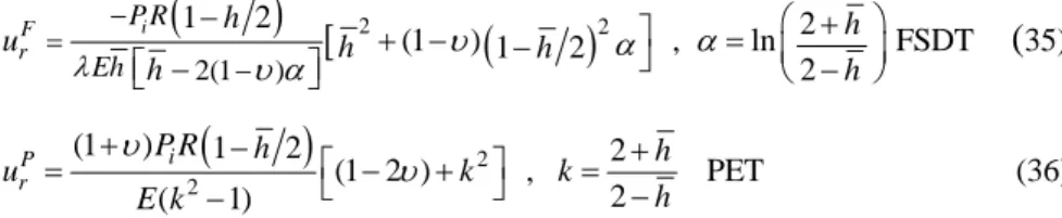
Fig. 3 shows that the radial displacement calculated by the two methods is almost identical at the middle surface domain and it increases at the inner surface; it is less than 4% anyway. In order to evaluate the effect of the wall thickness on the radial displacement, Eqs. (33) and (34) are expressed on the basis of h =h R.

( ) _[

²

( )

²

2(1 )

1 2 2

(1 ) 1 2 , ln FSDT

2

F i r

P R Eh

h h

u h h

h h

λ υ α α

υ α

= −

−

− + − − ⎤⎦ = ⎛⎜ + ⎞⎟

⎡ − ⎤ ⎝ − ⎠

⎣ ⎦

(

35)

( )

2

(1 ) 1 2 2

(1 2 ) , PET

( 1) 2

P i r

P R h h

u k k

E k h

υ υ

+ − ⎡ ⎤ +

= − ⎣ − + ⎦ = −

(36)

In Fig. 4, the percentage difference between FSDT and PET radial displacements

( )

(

^Diff ⁼ û^r^P⁻û^r^F û^r^P ^×¹⁰⁰

)

has been shown. This difference is increased with an increase in the thickness of the cylinder. The maximum difference occurs at 1 20≤h R≤16 20 and reaches15% , which is an acceptable value for the

(11)

analysis of thick cylinders. If the thickness of the wall equals radius of the middle surface

(

^h⁼^{1 ,}

)

the difference reaches25% .

Figure 3

Distribution of radial displacement in homogeneous cylinder

Figure 4

Difference percentages with respect to h=h R

5 Solution of the Heterogeneous Cylinders

In the isotropic heterogeneous cylinders, Poisson's ratio is constant and Young's modulus is calculated by inserting n in Eq. (8). In the current study, a range of

2 n 2

− ≤ ≤ is employed. By substituting stress components into Eqs. (18), the force and moment resultants are obtained. The matrices of coefficient in Eq. (19) are defined as the following form:

[ ] [ ]

[ ]

1 4 4 3 4 4

2 4 4

,

ij ij

ij

a Symmetric A c Symmetric A

b Antisymmetric A

× ×

×

⎧ =⎡ ⎤ =⎡ ⎤

⎪ ⎣ ⎦ ⎣ ⎦

⎨ = ⎡ ⎤

⎪ ⎣ ⎦

⎩

(37)

(12)

Constants in above relations are:

( )( )

(1 2 ) , ,

2

2 1

ln ln ,

2 2 2

o

i i

i

r r

k r K

r r

R h h k

R h k R h R h kr

μ υ

α β

⎧ = = = −

⎪⎪

⎨ ⎛ + ⎞ −

⎪ = ⎜ ⎟= = =

⎪ ⎝ − ⎠ + −

⎩

(38)

5.1 Inhomogeneity Constant of

n= −2 Elasticity modulus on the basis of Eq. (8) is:

( )

2

( ) 2

+ E ri i

E z

R z

=

(39)

Following above, nonzero components of the symmetric matrix

[ ]

^A_{1 4 4}_× ^are:

( )

( ) ( ) ( )

22 2 33

2

44 12 21

11

34 43

1 1

1

a ( ) R Rh a

a R Rh a a ( ) h R

a ( )

a a h R

υ υ α μα

μ α υ α

α

μ α

= − =

⎧ −

⎨ = − = = − −

⎩

= −

= = −

(40a)

and nonzero components of the antisymmetric matrix

[ ]

A2 4 4_× are:

( )

( ) ¹⁴ ⁴¹ ( )

( )

23 32

13 31

2

24 42

2

2 3

b b R

b b

b b h R h R R

υ υ α β

μα υ α β υ

β

μ α α β

= − = −

⎧⎪⎨ = − = − + −

⎪⎩

= − =

= − = − − + − + (40b)

and nonzero components of the symmetric matrix

[ ]

^A_{3 4 4}_× ^are:

2

22 33

2 2

44 34 43

1

2 1 1 1

4 4

c c ( )R

h

Rh h

c ( )R ( ) c c ( )

μα υ β

α υ β υ β υβ υ β

⎧ = − = − −

⎪⎪⎨

⎪ = − + + − − = = − + −

⎪⎩

(40c)

and the force vector { }_F _{4 1}_× is:

{ } ¹

{

⁰ ⁰ i o ²

(

i o

) }

^T

i i

P kP h P kP

F ⁼λE r ^{− +} ⁺

(40d)

Finally, the radial displacement on the basis of Eq. (25) is obtained as follows:

( ) (

²

)

²

2

1 (1 )

1 2(1 ) 2

i

r i o i o

Ei

u P kP P k P r r

R λ h

υβ υ β

υ

α β

= ⎧⎡ ⎤

− + − +

⎨⎢ ⎥

⎡ − ⎤ ⎩⎣ ⎦

⎢ ⎥

⎣ − ⎦

(13)

( ) (

²

)

2

i o i o

i

P kP P k P

r

α β ^⎫

+ − + + − ⎬

⎭

(41)

5.2 Inhomogeneity Constant of

n= +2 Elasticity modulus on the basis of Eq. (8) is:

( )

²

( ) 2ⁱ +

i

E z E R z

=r

(42) Following above, the nonzero components of the symmetric matrix

[ ]

^A_{1 4 4}_× ^are:

3 3 5

3 3

11 22 33

3 3 5 2 3 5 2 3 5

44 12 21 34 43

(1 ) (1 ) 3

12 80

4 4

3 (1 )

12 80 4 80 4 80

R h Rh

Rh Rh

a R h a a R h

R h Rh R h h R h h

a a a a a

υ υ μ

μ υ μ

⎧ = − ⎛⎜ + ⎞⎟ = − ⎛⎜ + ⎞⎟ = ⎛⎜ + ⎞⎟

⎪ ⎝ ⎠ ⎝ ⎠

⎪ ⎝ ⎠

⎨ ⎛ ⎞ ⎛ ⎞ ⎛ ⎞

⎪ = ⎜ + ⎟ = = − ⎜ + ⎟ = = ⎜ + ⎟

⎪ ⎝ ⎠ ⎝ ⎠ ⎝ ⎠

⎩

(43a)

and nonzero components of the antisymmetric matrix

[ ]

^A_{2 4 4}_× ^are:

3 3

2 3

13 31 14 41 23 32

3 2 3 5 2 3 5

3 3

24 42

5

12 12

6 4 80 3 40

4

h Rh

b b R h b b R h b b

Rh R h h R h h

Rh b b

R h

υ υ μ

υ μ υ

⎧ = − = ⎛⎜ + ⎞⎟ = − = ⎛⎜ + ⎞⎟ = − = −

⎪ ⎝ ⎠ ⎝ ⎠

⎪⎨

⎛ ⎞ ⎛ ⎞

⎛ ⎞

⎪×⎜ + ⎟+ = − = − ⎜ + ⎟+ ⎜ + ⎟

⎪ ⎝ ⎠ ⎝ ⎠ ⎝ ⎠

⎩

(43b)

and nonzero components of the symmetric matrix

[ ]

^A_{3 4 4}_× ^are:

3 3

22 33

3 3

3 2

44 34 43

(1 ) 4

(1 )

6 12

c R h Rh c Rh

Rh h

c R h c c R h

μ υ

υ υ

⎧ = − ⎛⎜ + ⎞⎟ = − −

⎪ ⎝ ⎠

⎪⎨

⎛ ⎞

⎪ = − − − = = −⎜ + ⎟

⎪ ⎝ ⎠

⎩

(43c)

and the force vector { }_F _{4 1}_× is:

{ } ⁱ³

{

⁰ ⁰ i o ²

(

i o

) }

^T

i

r P kP h P kP

F =λE − + +

(43d)

Finally, the radial displacement on the basis of Eq. (25) is obtained as follows:

(14)

( ) ( ) ( )

4 2

2 2

4 2 12

(1 2 )

144 6

i

r i o i o i i o

i

r E h

Rh h

u P kP P kP Rr P k P r

R h

h R

λ

υ υ

= ⎡⎢⎣ − − ⎛⎜⎝ + ⎞⎟⎠ ⎤ ⎣⎥⎦⎧⎡⎨⎩⎢ + + − + − ⎤⎥⎦

( ) ( )

2 2

4 ⁱ ^o 2 12 ⁱ ^o

i i

R h h h

R P kP R P kP

r r

⎡ ⎛ ⎞ ⎛ ⎞ ⎤⎫⎪

−⎢ ⎜ + ⎟ − + ⎜ + ⎟ + ⎥⎬

⎝ ⎠ ⎝ ⎠ ⎪

⎣ ⎦⎭ (44)

6 Numerical Analysis

The Finite Element Method (FEM) is a powerful numerical method in shell analysis. An axisymmetric thick cylindrical shell is studied in the field of the plane elasticity. In this field, it suffices to model only the shell section. An axisymmetric element has been applied for modeling and meshing. The degrees of freedom are two translations in the radial and axial direction for each node.

For the modeling of the FGM hollow cylinders, an innovative application for the multilayering of wall thickness in the radial direction has been performed. In this approach, N homogenous layers which are of identical thickness and step- variable elasticity modulus has been formed. The elasticity modulus of each layer is then calculated by the following relation:

( )

1

1 1 1 ,

N n

o i

j i

k r

j

E E k

N r

=

⎡ + − − ⎤

= ⎢ ⎥ =

⎣

∑

⎦

(45)

where N is the number of layers, n is the inhomogeneity constant and j is the number allocated to each layer. In our study, 20 layers have been used for modeling exercise.

The nodes are free in all the elements. However, in the boundaries of x=0 and x=L, to create plane strain conditions, nodes are free along the radius and the circumference, but are constrained along the length.

7 Discussions

As a case study, we consider a thick cylinder whose elasticity modulus varies in radial direction and has the following characteristics: r_i=40mm, r_o =60 mm, Young's modulus of inner surface E_i=200 GPa and Poisson's ratio υ=0.3. Fig.

5 shows the distribution of elasticity modulus with respect to the normalized radius in a heterogeneous cylinder for integer values of n.

(15)

7.1 Internal Pressure

In this section, consider a nonhomogeneous thick cylinder in which the inner surface is compressed by uniform pressure P_i= =P 80 MPa and the outer surface is traction free. The distribution of the normalized radial displacement of this cylinder is depicted in Fig. 6. It is seen that for negative values of n, the displacements of FGM cylinders are higher than of a homogeneous cylinder. For positive values of n, the situation is reverse, i.e. the displacement is lower. The variation in the displacement of heterogeneous material is similar to that of homogenous material.

Figure 5

Distribution of elasticity modulus in FGM cylinder

Figure 6

Distribution of radial displacement in FGM cylinder (P_i=80 MPa)

Fig. 7 illustrates the distribution of normalized circumferential stress in a FGM cylinder. It should be pointed out that the equivalent graphs in Ref. (Tutuncu, 2001) are incorrect. For n<0, in the inner half of the cylinder, the amount of circumferential stress is higher than that of the homogeneous cylinder. In contrast, in the outer half, it is lower. For n>0, the situation is reverse. In the inner half of the cylinder, the amount of circumferential stress is lower than that of the homogeneous cylinder. As opposed to this, in the outer half, it is higher. In the

(16)

domain of the middle surface, the behavior of a FGM cylinder is similar to homogenous cylinder. The numerical results of this study are presented in Tables 1 and 2.

Figure 7

Distribution of circumferential stress in FGM cylinder (P_i=80 MPa) Table 1

Numerical results of radial displacement (Pi =80 MPa)

Surface u_r , mm n= -2 n= -1 n= 0 n= +1 n= +2 FSDT 0.054309 0.045790 0.038096 0.031266 0.025312

PET 0.054541 0.045989 0.038272 0.031426 0.025458 Middle

surface

FEM 0.054559 0.045997 0.038272 0.031426 0.025458 FSDT 0.060512 0.050984 0.042388 0.034764 0.028124 PET 0.062163 0.052673 0.044096 0.036471 0.029811 Inner

surface

FEM 0.062182 0.052680 0.044096 0.036468 0.029806

Table 2

Numerical results of maximum stress (Pi =80 MPa)

Surface σ_θ,^MPa n= -2 n= -1 n= 0 n= +1 n= +2

FSDT 141.35 149.30 155.62 160.00 162.36

PET 148.99 151.08 156.16 159.31 159.81 Middle

surface

FEM 144.29 151.15 156.16 159.12 159.80

FSDT 335.72 283.23 235.78 193.63 156.85

PET 307.27 255.13 208 166.11 129.51 Inner

surface

FEM 299.91 252.09 208 168.18 133.60

7.2 External Pressure

In this section, consider a nonhomogeneous thick cylinder in which the outer surface is compressed by uniform pressure P_o= =P 80 MPa and the inner surface is traction free.

(17)

Figure 8

Distribution of radial displacement in FGM cylinder (P_o=80 MPa)

The distribution of the normalized radial displacement of this cylinder is depicted in Fig. 8. It is seen that for negative values of n, the displacements of FGM cylinders are higher than of a homogeneous cylinder. For positive values of n, the situation is reverse, i.e. the displacement is lower. The variation in the displacement of homogenous material is similar to that of heterogeneous material.

Figure 9

Distribution of circumferential stress in FGM cylinder (P_o=80 MPa)

Fig. 9 illustrates the distribution of normalized circumferential stress in a FGM cylinder. For n<0, in the inner half of the cylinder, the amount of circumferential stress is higher than that of the homogeneous cylinder. In contrast, in the outer half, it is lower. For n>0, the situation is reverse. In the inner half of the cylinder, the amount of circumferential stress is lower than that of the homogeneous cylinder. As opposed to this, in the outer half, it is higher. In the domain of the middle surface, the behavior of a FGM cylinder is similar to homogenous cylinder. The numerical results of this study are presented in Tables 3 and 4.

(18)

Table 3

Numerical results of radial displacement (Po =80 MPa)

Surface ur , mm n= -2 n= -1 n= 0 n= +1 n= +2 FSDT -0.069367 -0.058383 -0.048496 -0.039745 -0.032136

PET -0.069714 -0.058630 -0.048672 -0.039872 -0.032228 Middle

surface

FEM -0.069737 -0.058640 -0.048675 -0.039871 -0.032227 FSDT -0.072159 -0.060894 -0.050707 -0.041653 -0.033749 PET -0.074801 -0.063030 -0.052416 -0.043005 -0.034809 Inner

surface

FEM -0.074821 -0.063037 -0.052416 -0.043002 -0.034806 Table 4

Numerical results of maximum stress (Po =80 MPa)

Surface σ_θ,^MPa n= -2 n= -1 n= 0 n= +1 n= +2 FSDT -218.44 -228.32 -235.62 -240 -241.29

PET -221.87 -230.20 -236.16 -239.43 -239.81 Middle

surface

FEM -222.03 -230.28 -236.16 -239.42 -239.80 FSDT -453.47 -380.89 -315.79 -258.34 -208.54 PET -411.0 -346.32 -288 -236.29 -191.26 Inner

surface

FEM -401.0 -342.07 -288 -239.22 -196.04 Conclusions

In this research, the heterogeneous hollow cylinders have been solved by FSDT, PET and FEM, and have been compared with homogenous cylinders. We conclude that for the positive or negative values of n, the maximum stress increases in one half of the cylinder, and it is decreased in the other half. The radial displacement for positive values of n is decreases; it is however increased for negative values. As n is increases, the amount of changes in both displacements and stresses increases too. Therefore, positive values of n lead to a decrease in the displacement and stress in the inner surface. This is highly important for a large number of industries.

Acknowledgement

The authors wish to thank Dr. Kazemi for his kind cooperation.

References

[1] Koizumi, M.: The Concept of FGM, Ceramic Transactions Functionally Graded Material, Vol. 34, pp. 3-10, 1993

[2] Naghdi, P. M. and Cooper, R. M.: Propagation of Elastic Waves in Cylindrical Shells Including the Effects of Transverse Shear and Rotary Inertia, Journal of the Acoustical Society of America, Vol. 28, No. 1, pp.

56-63, 1956

(19)

[3] Mirsky, I. and Hermann, G.: Axially Motions of Thick Cylindrical Shells, Journal of Applied Mechanics, Vol. 25, pp. 97-102, 1958

[4] Mindlin, R. D.: Influence of Rotary Inertia and Shear on Flexural Motions of Isotropic Elastic Plates, Journal of Applied Mechanics, Vol. 18, pp. 31- 38, 1951

[5] Greenspon, J. E.: Vibration of a Thick-walled Cylindrical Shell, Camparison of the Exact Theory with Approximate Theories, Journal of the Acoustical Society of America, Vol. 32, No. 5, pp. 571-578, 1960

[6] Ziv, M. and Perl, M.: Impulsive Deformation of Mirsky-Hermann's Thick Cylindrical Shells by a Numerical Method, Journal of Applied Mechanics, Vol. 40, No. 4, pp. 1009-1016, 1973

[7] Suzuki, K., Konnon, M. and Takahashi, S.: Axisymmetric Vibration of a Cylindrical Shell with Variable Thickness, JSME, Vol. 24, No. 198, pp.

2122-2132, 1981

[8] Simkins, T. E.: Amplifications of Flexural Waves in Gun Tubes, Journal of Sound and Vibration, Vol. 172, No. 2, pp. 145-154, 1994

[9] Eipakchi, H. R., Rahimi, G. H. and Khadem, S. E.: Closed Form Solution for Displacements of Thick Cylinders with Varying Thickness Subjected to Non-Uniform Internal Pressure, Structural Engineering and Mechanics, Vol. 16, No. 6, pp. 731-748, 2003

[10] Ghannad, M. and Nejad, M. Z.: Elastic Analysis of Pressurized Thick Hollow Cylindrical Shells with Clamped-Clamped Ends, Mechanika, Vol.

85, pp. 11-18, 2010

[11] Fukui, Y. and Yamanaka, N.: Elastic Analysis for Thick-walled Tubes of Functionally Graded Materials Subjected to Internal Pressure, JSME Ser. I, Vol. 35, No. 4, pp. 891-900, 1992

[12] Horgan, C. O. and Chan, A. M.: The Pressurized Hollow Cylinder or Disk Problem for Functionally Graded Isotropic Linearly Elastic Materials, Journal of Elasticity, Vol. 55, No. 1, pp. 43-59, 1999

[13] Tutuncu, N. and Ozturk, M.: Exact Solutions for Stresses in Functionally Graded Pressure Vessels, Composites Part B-Engineering, Vol. 32, No. 8, pp. 683-686, 2001

[14] Hongjun, X., Zhifei, S. and Taotao, Z.: Elastic Analyses of Heterogeneous Hollow Cylinders, Mechanics Research Communications, Vol. 33, No. 5, pp. 681-691, 2006

[15] Zhifei, S., Taotao, Z. and Hongjun, X.: Exact Solutions of Heterogeneous Elastic Hollow Cylinders, Composite Structures, Vol. 79, No. 1, pp. 140- 147, 2007

(20)

[16] Tutuncu, N.: Stresses in Thick-walled FGM Cylinders with Exponentially- Varying Properties, Engineering Structures, Vol. 29, No. 9, pp. 2032-2035, 2007

[17] Nejad, M. Z., Rahimi, G. H. and Ghannad, M.: Set of Field Equations for Thick Shell of Revolution Made of Functionally Graded Materials in Curvilinear Coordinate System, Mechanika, Vol. 77, No. 3, pp. 18-26, 2009

[18] Ghannad, M., Rahimi, G. H. and Khadem, S. E.: General Plane Elasticity Solution of Axisymmetric Functionally Graded Thick Cylindrical Shells, Journal of Modares Technology and Engineering, Vol. 10, pp. 31-43, 2010 [19] Abedi, M., Nejad, M. Z., Lotfian, M. H. and Ghannad, M.: Static Analysis

of Parabolic FGM Solid Cylinders, Journal of Basic and Applied Scientific Research, Vol. 1, No. 11, pp. 2339-2345, 2011

[20] Wylie, C. R.: Differential Equations, McGraw-Hill, New York, 1979

[21] Vlachoutsis, S.: Shear Correction Factors for Plates and Shells, International Journal for Numerical Methods in Engineering, Vol. 33, No.

7, pp. 1537-1552, 1992

Elastic Analysis of Heterogeneous Thick Cylinders Subjected to Internal or External Pressure Using Shear Deformation Theory