Failure Prediction Models for Accelerated Life Tests
VIVIEN SIPKÁS, GABRIELLA BOGNÁR Institute of Machine and Product Design
University of Miskolc
3515 Miskolc, Miskolc-Egyetemváros HUNGARY
machsv@uni-miskolc.hu, v.bognar.gabriella@uni-miskolc.hu
Abstract: The aim of this paper is to introduce the reliability methods in connection with lifetime determination and to design testing method for the prediction of the life of the micro switches. These products are subjected to complex stressing, for example, humidity, temperature, current load and so on. Therefore, the most important failure prediction methods, acceleration life testing methods with one, two or more variables have been introduced, as these methods are essential and necessary for reliability prediction.
Key-Words: Accelerated Life Testing, Lifetime, Bathtub Curve, Failure Prediction, Reliability Prediction, Arrhenius Relationship
1 Introduction
We shall understand the reliability that a product maintains its initial quality and performance at a certain period of time, cycle, distance etc. under given conditions without failure. The operating conditions could be environmental conditions and working conditions. Environmental conditions include the humidity, vibration and temperature.
The working condition means an artificial environment such as voltage, current load, place for installment and hours of use, which occurs during the life of the product [1].
It has already been pointed out in our previous papers that unfortunately the micro switches used in gardening machines have several malfunctions.
During the last few years it was practiced, that certain types of micro switches have not provided a desirable life. Among others, due to high temperatures, deformation of internal components, loss of function, switching and breaking of button switches have experienced. In addition, the material surface can be burned and the contacting surfaces can be charred. For all of these reasons, the switch will not work properly [7-9]. Therefore, it is necessary to develop different test methods to predict the life expectancy of products.
The aim our investigations is to carry out pre- planned measurements and testing micro switches applied in several types of garden tools. To obtain objective conclusions, we need an effective method for designing and analyzing the experiments.
2 Failure prediction
The reliability prediction is to predict failure rate and average life span associated with reliability by taking operation, working environment and conditions associated with systems and parts into account.
The prediction will eventually be used mainly in design and product development stage of parts and system. Also, the prediction enables the operators to secure customer safety by building preventive maintenance plan in advance.
Predicting the life span of parts and applying it to maintenance or conducting activities to promote longer life span by reflecting operation data feedback to a design are not yet a common practice and it is quite challenging [1, 4-6].
2.1 The Bathtub Curve
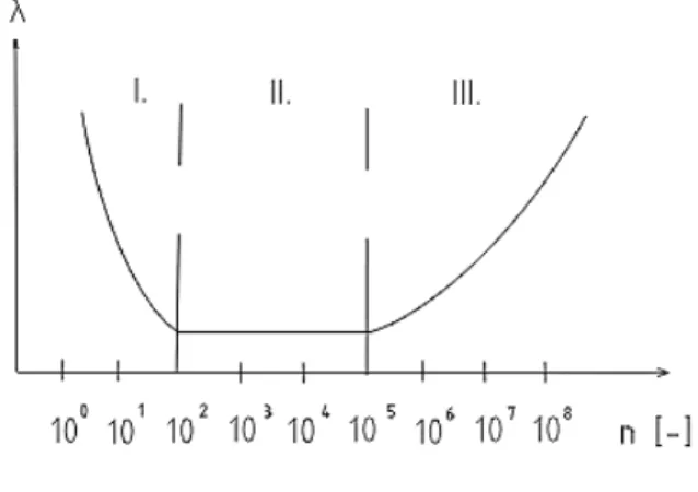
We have already described in detail in our previous articles the bathtub curve’s features and the bathtub shape’s three phases of life for components, which was predicted by physics of failures (see Fig.1., [3, 7-9]).
2.1.1 Early, infant failures (I.)
In this is early life that is mortality, which is characterized by decreasing failure rate.
2.1.2 Middle, random phase (II.)
In this phase useful life, which has relatively constant failure rate.
2.1.3. Usage, wear out phase (III.)
The last phase is the long-term wear–out segment, which increases rapidly with increasing failure rate [3, 4].
Figure 1. The bathtub curve
2.2 Failure-Time Distribution Functions
The probability distribution for failure time T can be characterized by a cumulative distribution function, probability density function, a survival or hazard function. These functions are described below and illustrated for typical failure-time distributions.These functions are exhibited in the diagrams. The choice of function to use depends on convenience of model specification, interpretation, or technical development; all these functions are important for one or another purpose. On Figs. 2-4, we show the cumulative distribution function, the probability density function and the hazard function [2].
Figure 2. Cumulative distribution function
Figure 3. Probability Density function
Figure 4. Hazard Function
Applying the general three-parameter form of the Weibull distribution, the distribution function can be formulated as a follow [7-9]:
𝐹𝐹(𝑡𝑡) =�1− 𝑒𝑒𝑒𝑒𝑒𝑒 �−(𝑡𝑡 − 𝛾𝛾) 𝛼𝛼
𝛽𝛽
�,𝑖𝑖𝑖𝑖 𝑡𝑡 ≥ 𝛾𝛾, 0 ,𝑖𝑖𝑖𝑖 𝑡𝑡<𝛾𝛾.
(1)
Function F(t) gives the failure probability during the actual operating time. In formula (1) the statistical variable is time t in hours or number of operations, the parameters involved in (1) are the following:
α> 0 is the scalar parameter, β> 0 is the shape parameter, γ≥ 0 is the location parameter.
The characteristic lifetime is denoted by 𝜂𝜂. Let us introduce the substitution 𝜂𝜂 =𝛼𝛼1/𝛽𝛽 into expression (1). Thus, the distribution function can be written as follows:
𝐹𝐹(𝑡𝑡) =�1− 𝑒𝑒𝑒𝑒𝑒𝑒 �− �𝑡𝑡 − 𝛾𝛾 𝜂𝜂 �
𝛽𝛽�,𝑖𝑖𝑖𝑖 𝑡𝑡 ≥ 𝛾𝛾, 0, 𝑖𝑖𝑖𝑖 𝑡𝑡<𝛾𝛾.
(1𝑎𝑎)
The position parameter γ can be taken to 0 for a few practical applications, the sampling plans are designed for case γ=0. The shape parameter β determines the figure of the density function. The density function f(t) for the Weibull distribution with γ=0 can be determined by differentiation from the formula (1a) (see Fig. 2).
𝑖𝑖(𝑡𝑡) =𝐹𝐹′(𝑡𝑡)
=� 𝛽𝛽
𝜂𝜂 � 𝑡𝑡 𝜂𝜂�
𝛽𝛽−1 𝑒𝑒𝑒𝑒𝑒𝑒 �− �𝑡𝑡 𝜂𝜂�
𝛽𝛽�,𝑖𝑖𝑖𝑖 𝑡𝑡 ≥0, 0, 𝑖𝑖𝑖𝑖 𝑡𝑡< 0. (2) If β<1, then f(t) is a monotone decreasing function, this is the phase of early failures.
If β=1, then we get the exponential distribution, which is the phase of random failures.
If β>1, then density function has a maximum, this characterize the phase-related failure phase [7-9].
Figure 5. The density function of the Weibull distribution for different values of β
2.3 Electronic Parts Failure Prediction
The reliability test can be qualified by single component, but as more and more components are integrated altogether to form a desired electronic module, the individual components can be reduced due to interaction with overall system design [3].
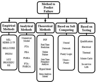
There are several type of failure predictions which can be used in the industrial development. Figure 6.
represents some of these methods, which are further classified into different groups based on several technologies.
It can be deducted from the Fig. 6. that there are many types of methods. We shall introduce some of them in more detail, which are most likely to be applied for micro switches at the current stage of the research.
Figure 6. Failure prediction methods [3]
2.3.1 Empirical methods
The type of these methods based on models to predict the failure developed from historical data collected from filed, manufacturer or test data, is called empirical methods. These types of evaluations are widely used in military, automotive and commercial use. Also, it is easy to use, it provides relatively good performance and approximation of field failure rates, but the data used is not device specific, so approximation cannot be perfect [10, 11]
2.3.2 Analytical methods
To predict the failure, the analytical methods provide better approximation. Various numerical models are used to predict the failure. Finite Element Method (FEM) is an accurate technique for fault prediction, as it deals with both normal and faulty characteristics of the device. Fault tree analysis (FTA) is a numerical approach to detect fault based on the simulation. Failure mode, mechanisms and effect analysis (FMMEA) is a systematic and anticipatory method that deals with step by step approach to identify the faults during design or in service. A modified approach was discussed, which is a hybrid of FTA and FMECA and identifies and estimates the effects of failure (see [3]).
2.3.3 Theoretical methods
Physics of failure understands the failure mechanism and different models of physics can be applied for the data. For accurate prediction of wear out failure of components, analysis is costly, complex and detailed manufacturing characteristics
of component are needed. Physics of failure can be used both at design stage and at the production stage.
2.3.4 Methods based on soft computing techniques
Some authors have also applied a soft computing approach (neuro-fuzzy model) for intelligent online performance monitoring of electronic circuits and devices and classifies the stressors broadly into three main groups: electrical stressors, mechanical stressors and thermal environment of the component.
2.3.5 Failure prediction method based on testing
In life data analysis or Weibull analysis, under normal operating conditions reliability is measured using a test which is conducted on large sample of units, time-to-failure are analyzed using statistical distribution. Due to design or manufacturing, the components are not independent, but physics of failure and empirical method assumes that there is no interaction between failures, so for realistic prediction at system level, life testing method is preferred over physics of failure or empirical method.
3 Acceleration life testing with one variable factor
Today’s manufacturers face strong pressure to develop new products with higher technological content in record time while improving productivity, product field reliability and overall quality. This has motivated the development of such methods like concurrent engineering and has encouraged us to design experiments for product and process improvement. The requirements for higher reliability have increased the need of testing the materials, the components and the systems. To achieve high reliability, it is necessary to improve the design and manufacturing processes.
In the literature we can find three different methods of accelerated reliability tests [3]:
i.) Increase the use-rate of the product.
Useful reliability information could be obtained in a matter of days instead of months.
ii.) Increase the aging-rate of the product.
Increasing the level of experimental variables like temperature or humidity we can accelerate the chemical processes of certain failure mechanisms.
iii.) Increase the level of stress.
In the last type we increase the level of stress, the temperature, the voltage, or the pressure during the tests comparing with the levels that units operate. A unit will fail when its strength drops below applied stress. Thus, a unit at a high stress will generally fail more rapidly than it would have failed at low stress.
Combination of these methods of acceleration are also employed. Variable like voltage and temperature cycling can both rate of an electrochemical reaction and increase stress relative to strength. In those situations, when the effect of an accelerating variable is complicated, there may not be enough, physical model for acceleration[3].
Combination of these methods will be used further of the research, because the micros witches will also be subjected to complex stresses.
3.1 Use Rate
Increasing use-rate will, for some components, accelerate failure causing wear and degradation. The increased use rate attempts to simulate actual use.
Therefore, other environmental factors should be controlled to mimic actual use environments.
For example:
• Running automobile engines, appliances, and similar products and continuously or with higher than usual-rates.
• Higher than usual cycling rates for relays and switches.
• Increasing the cycling rate (frequency) in fatigue testing.
There is a basic assumption underlying simple use- rate acceleration models. Useful life must be adequately modeled by cycles of operation and cycling rate or frequency should not impact on the cycles-to-failure distribution. This is reasonable if cycling return to steady state after each cycle [2, 12].
3.2 Temperature Acceleration
Increasing temperature is one of the most commonly used methods to accelerate a failure mechanism.
The Arrhenius relationship is a widely used model describing the effect that temperature has on the rate of a simple chemical reaction. This relationship can be written as
ℛ(𝑡𝑡𝑒𝑒𝑡𝑡𝑒𝑒) =� −𝐸𝐸𝑎𝑎
𝑘𝑘𝑏𝑏 x 𝑡𝑡𝑒𝑒𝑡𝑡𝑒𝑒 𝐾𝐾�
=𝛾𝛾0𝑒𝑒𝑒𝑒𝑒𝑒 �−𝐸𝐸𝑎𝑎 x 11605
𝑡𝑡𝑒𝑒𝑡𝑡𝑒𝑒 𝐾𝐾 �, (3) where ℛ is the reaction rate at 𝑡𝑡𝑒𝑒𝑡𝑡𝑒𝑒 𝐾𝐾= 𝑡𝑡𝑒𝑒𝑡𝑡𝑒𝑒 ° 𝐶𝐶+ 273,15 is temperature in the absolute Kelvin scale, 𝑘𝑘𝑏𝑏 = 8,6171 𝑒𝑒 10−5 1/11605 is Boltzmann’s constant [electron volts per ° 𝐶𝐶], and 𝐸𝐸𝑎𝑎 is the activation energy in electron volts [eV]. The parameters 𝐸𝐸𝑎𝑎and 𝛾𝛾0 are product or material characteristics. The Arrhenius acceleration factor for the use temperature 𝑡𝑡𝑒𝑒𝑡𝑡𝑒𝑒𝑈𝑈 is
𝒜𝒜ℱ( 𝑡𝑡𝑒𝑒𝑡𝑡𝑒𝑒, 𝑡𝑡𝑒𝑒𝑡𝑡𝑒𝑒𝑈𝑈, 𝐸𝐸𝑎𝑎) =ℛ( 𝑡𝑡𝑒𝑒𝑡𝑡𝑒𝑒ℛ(𝑡𝑡𝑒𝑒𝑡𝑡𝑒𝑒𝑈𝑈 ))= exp� 𝐸𝐸𝑎𝑎� 𝑡𝑡𝑒𝑒𝑡𝑡𝑒𝑒11605
𝑈𝑈 𝐾𝐾−𝑡𝑡𝑒𝑒𝑡𝑡𝑒𝑒11605 𝐾𝐾�� (4) When 𝑡𝑡𝑒𝑒𝑡𝑡𝑒𝑒 > 𝑡𝑡𝑒𝑒𝑡𝑡𝑒𝑒𝑈𝑈, then 𝒜𝒜ℱ� 𝑡𝑡𝑒𝑒𝑡𝑡𝑒𝑒, 𝑡𝑡𝑒𝑒𝑡𝑡𝑒𝑒𝑈𝑈, 𝐸𝐸𝑎𝑎�> 1. When 𝑡𝑡𝑒𝑒𝑡𝑡𝑒𝑒𝑈𝑈 and 𝐸𝐸𝑎𝑎 are understood to be, respectively, product use temperature and reaction – specific activation energy 𝒜𝒜ℱ (𝑡𝑡𝑒𝑒𝑡𝑡𝑒𝑒) =𝒜𝒜ℱ( 𝑡𝑡𝑒𝑒𝑡𝑡𝑒𝑒, 𝑡𝑡𝑒𝑒𝑡𝑡𝑒𝑒𝑈𝑈, 𝐸𝐸𝑎𝑎) will be used to denote a time-acceleration factor
𝒜𝒜ℱ� 𝑡𝑡𝑒𝑒𝑡𝑡𝑒𝑒𝐻𝐻𝑖𝑖𝐻𝐻ℎ , 𝑡𝑡𝑒𝑒𝑡𝑡𝑒𝑒𝐿𝐿𝐿𝐿𝐿𝐿, 𝐸𝐸𝑎𝑎�
= exp( 𝐸𝐸𝑎𝑎 x 𝑇𝑇𝑇𝑇𝐹𝐹) (5) as a function of 𝐸𝐸𝑎𝑎 and the temperature differential factor (TDF) values (see [2])
𝑇𝑇𝑇𝑇𝐹𝐹=� 11605
𝑡𝑡𝑒𝑒𝑡𝑡𝑒𝑒𝐿𝐿𝐿𝐿𝐿𝐿 𝐾𝐾 −
11605
𝑡𝑡𝑒𝑒𝑡𝑡𝑒𝑒𝐻𝐻𝑖𝑖𝐻𝐻ℎ 𝐾𝐾�. (6) The Arrhenius relationship does not apply to all temperature-acceleration problems and will be adequate over only limited temperature range (depending on the particular application). Even dough, it is satisfactorily and widely used in many applications [12].
3.3 Pressure Acceleration
Increasing voltage or voltage stress (electric field) is another commonly used method to accelerate failure of electrical materials and components like light bulbs, capacitors, transformers, heaters, and insulation. Voltage is defined as the difference in electrical potential between two points. Physically it can be thought of as the amount of pressure behind an electrical current. Voltage stress across a dielectric is measured in units of volts/thickness.
3.3.1. Inverse-power acceleration
The most commonly used model for voltage acceleration is the inverse power relationship.
Let 𝑇𝑇(𝑣𝑣𝐿𝐿𝑣𝑣𝑡𝑡) and 𝑇𝑇(𝑣𝑣𝐿𝐿𝑣𝑣𝑡𝑡𝑈𝑈) denote the failure times that would result for a particular unit tested at increased voltage and use voltage conditions, respectively. The inverse power relationship is the following:
𝑇𝑇(𝑣𝑣𝐿𝐿𝑣𝑣𝑡𝑡) = 𝑇𝑇(𝑣𝑣𝐿𝐿𝑣𝑣𝑡𝑡𝑈𝑈)
𝒜𝒜ℱ(𝑣𝑣𝐿𝐿𝑣𝑣𝑡𝑡) =�𝑣𝑣𝐿𝐿𝑣𝑣𝑡𝑡
𝑣𝑣𝐿𝐿𝑣𝑣𝑡𝑡𝑈𝑈�𝛽𝛽1𝑇𝑇(𝑣𝑣𝐿𝐿𝑣𝑣𝑡𝑡𝑈𝑈), (7) which is the scale-accelerated failure-time (SAFT) model. The relationship in the formula (7) is known as the inverse power relationship, since generally 𝛽𝛽1< 0.
The inverse power relationship voltage-acceleration factor can be expressed as
𝒜𝒜ℱ(𝑣𝑣𝐿𝐿𝑣𝑣𝑡𝑡) =𝒜𝒜ℱ� 𝑡𝑡𝑒𝑒𝑡𝑡𝑒𝑒, 𝑡𝑡𝑒𝑒𝑡𝑡𝑒𝑒𝑈𝑈, 𝛽𝛽1�=𝑇𝑇(𝑣𝑣𝐿𝐿𝑣𝑣𝑡𝑡𝑈𝑈) 𝑇𝑇(𝑣𝑣𝐿𝐿𝑣𝑣𝑡𝑡)
=�𝑣𝑣𝐿𝐿𝑣𝑣𝑡𝑡
𝑣𝑣𝐿𝐿𝑣𝑣𝑡𝑡𝑈𝑈�−𝛽𝛽1. (8)
When 𝑣𝑣𝐿𝐿𝑣𝑣𝑡𝑡>𝑣𝑣𝐿𝐿𝑣𝑣𝑡𝑡𝑈𝑈 and 𝛽𝛽1< 0, 𝒜𝒜ℱ� 𝑡𝑡𝑒𝑒𝑡𝑡𝑒𝑒, 𝑡𝑡𝑒𝑒𝑡𝑡𝑒𝑒𝑈𝑈, 𝛽𝛽1�>1. When 𝑣𝑣𝐿𝐿𝑣𝑣𝑡𝑡𝑈𝑈 and 𝛽𝛽1 are understood to be, respectively, product use voltage and the material-specific exponent, 𝒜𝒜ℱ� 𝑡𝑡𝑒𝑒𝑡𝑡𝑒𝑒, 𝑡𝑡𝑒𝑒𝑡𝑡𝑒𝑒𝑈𝑈, 𝛽𝛽1� denotes the acceleration factor. 𝒜𝒜ℱ as a function of stress ratio and 𝛽𝛽1 [12].
4 Acceleration models with two accelerating factors
In some accelerated tests more than one accelerating variable are used. Such tests might be suggested when it is known that two or more potential accelerating variables exist.
For example, the two variable accelerated lifetime test (ALT) model, for long-location-scale distribution, the two-variable model is applied. The linear function µ of two experimental variables:
𝜇𝜇 =𝜇𝜇(𝑒𝑒1,𝑒𝑒2) =𝛽𝛽0+𝛽𝛽1𝑒𝑒1+𝛽𝛽2𝑒𝑒2, (9) where 𝑒𝑒1 and 𝑒𝑒2 are the possibly transformed levels of the accelerating or other experimental variables and 𝛽𝛽0,𝛽𝛽1,𝛽𝛽2 are unknown coefficients to be estimated from test data. In some under underlying failure processes, it is possible for the underlying accelerating variables to interact. For example, in the model
𝜇𝜇=𝜇𝜇(𝑒𝑒1,𝑒𝑒2) =𝛽𝛽0+𝛽𝛽1𝑒𝑒1+𝛽𝛽2𝑒𝑒2+𝛽𝛽3𝑒𝑒1𝑒𝑒2 (10) the transformed variables are 𝑒𝑒1 and 𝑒𝑒2 interact in the sense that the effect of changing 𝑒𝑒1 depends on the level of 𝑒𝑒2and vice versa [12]. Parameters 𝛽𝛽𝑖𝑖 are unknown that are characteristics of the material or product being tested and they are to be estimated from the available ALT.
4.1 Temperature–(voltage) Stress Acceleration
The terms with 𝑒𝑒1 and 𝑒𝑒2 correspond, respectively, to the Arrhenius and the power relationship acceleration models. The term with 𝑒𝑒3, a function of both temperature and voltage, is an interaction suggesting that the temperature – acceleration factor depends on the level of voltage. Similarly, a voltage-temperature interaction suggests that the voltage-acceleration factor depends on the level of temperature [2, 12].
ℛ(𝑡𝑡𝑒𝑒𝑡𝑡𝑒𝑒,𝑣𝑣𝐿𝐿𝑣𝑣𝑡𝑡)
=𝛾𝛾0 𝑒𝑒 (𝑡𝑡𝑒𝑒𝑡𝑡𝑒𝑒 𝐾𝐾)𝑡𝑡 x exp�𝑘𝑘𝐵𝐵x 𝑡𝑡𝑒𝑒𝑡𝑡𝑒𝑒 𝐾𝐾�−𝐸𝐸𝑎𝑎
x exp�𝛾𝛾2log(𝑣𝑣𝐿𝐿𝑣𝑣𝑡𝑡) +𝛾𝛾3log(𝑣𝑣𝐿𝐿𝑣𝑣𝑡𝑡)
𝑘𝑘𝐵𝐵 x 𝑡𝑡𝑒𝑒𝑡𝑡𝑒𝑒 𝐾𝐾� , (11) where the 𝑒𝑒1 = 11605/𝑡𝑡𝑒𝑒𝑡𝑡𝑒𝑒𝐾𝐾, 𝑒𝑒2= log(𝑣𝑣𝐿𝐿𝑣𝑣𝑡𝑡), 𝑒𝑒3=𝑒𝑒1𝑒𝑒2.
The failure time T gives [12]
𝑇𝑇(𝑡𝑡𝑒𝑒𝑡𝑡𝑒𝑒,𝑣𝑣𝐿𝐿𝑣𝑣𝑡𝑡) = 1
ℛ(𝑡𝑡𝑒𝑒𝑡𝑡𝑒𝑒,𝑣𝑣𝐿𝐿𝑣𝑣𝑡𝑡)�𝑣𝑣𝐿𝐿𝑣𝑣𝑡𝑡
𝛿𝛿0 �𝛾𝛾1. (12) Then, the ratio of failure times at (𝑡𝑡𝑒𝑒𝑡𝑡𝑒𝑒𝑈𝑈,𝑣𝑣𝐿𝐿𝑣𝑣𝑡𝑡𝑈𝑈) versus (𝑡𝑡𝑒𝑒𝑡𝑡𝑒𝑒,𝑣𝑣𝐿𝐿𝑣𝑣𝑡𝑡) is the acceleration factor
𝒜𝒜ℱ(𝑡𝑡𝑒𝑒𝑡𝑡𝑒𝑒,𝑣𝑣𝐿𝐿𝑣𝑣𝑡𝑡) =𝑇𝑇(𝑡𝑡𝑒𝑒𝑡𝑡𝑒𝑒𝑈𝑈,𝑣𝑣𝐿𝐿𝑣𝑣𝑡𝑡𝑈𝑈) 𝑇𝑇(𝑡𝑡𝑒𝑒𝑡𝑡𝑒𝑒,𝑣𝑣𝐿𝐿𝑣𝑣𝑡𝑡)
=𝑒𝑒𝑒𝑒𝑒𝑒[𝐸𝐸𝑎𝑎(𝑒𝑒1𝑈𝑈
− 𝑒𝑒1)] x (𝑣𝑣𝐿𝐿𝑣𝑣𝑡𝑡
𝑣𝑣𝐿𝐿𝑣𝑣𝑡𝑡𝑈𝑈 )𝛾𝛾2−𝛾𝛾1x {𝑒𝑒𝑒𝑒𝑒𝑒[𝑒𝑒1𝑣𝑣𝐿𝐿𝐻𝐻(𝑣𝑣𝐿𝐿𝑣𝑣𝑡𝑡)
− 𝑒𝑒1𝑈𝑈log(𝑣𝑣𝐿𝐿𝑣𝑣𝑡𝑡𝑈𝑈)]}𝛾𝛾3, (13) where 𝑒𝑒1𝑈𝑈 = 11605/(𝑡𝑡𝑒𝑒𝑡𝑡𝑒𝑒𝑈𝑈𝐾𝐾) and 𝑒𝑒1= 11605/𝑡𝑡𝑒𝑒𝑡𝑡𝑒𝑒𝐾𝐾. For the special case when 𝛾𝛾3= 0 (no interaction), 𝒜𝒜ℱ(𝑡𝑡𝑒𝑒𝑡𝑡𝑒𝑒,𝑣𝑣𝐿𝐿𝑣𝑣𝑡𝑡) is composed of separate factors for temperature and voltage acceleration. The voltage-acceleration factor (holding temperature constant) does not depend on the temperature level used in the acceleration.
4.2 Temperature – Humidity Acceleration
Humidity is commonly used accelerating variable, particularly for failure mechanisms involving corrosion and certain kinds of chemical degradation [2, 12].A variety of humidity models, mostly empirical but few with some physical basis have been suggested for different kinds of failure mechanisms. humidity is also an important factor in the service-life in distribution. In most test applications, where humidity is used as an accelerated variable, it used in conjunction with temperature.
5 Acceleration Life Testing More Than Two Experimental Variables
For more different units to be tested, we may need the acceleration life testing with more than two experimental variables, and prediction processes to summarize the influences.
In the applications it is often necessary or useful to conduct an accelerated test with more than two experimental variables. In such situations the ideas presented in this chapter can be extended and combined with traditional experimental design concepts [2, 12].
When the number of nonaccelerating variables is more than two or three, complete factorial designs may lead to an unreasonably large number of variable-level combinations. In this case, a reasonable strategy would be to use a standard fraction of a factorial design for the nonaccelerating variables and to run a single-variables ALT compromise plan at each of the combinations in the fraction.
6 Conclusion
In this paper the most important type of failure prediction methods has been considered. These methods are important and useful to apply in the prediction of lifetime with accelerated lifetime test.
Here, the acceleration models with one, two or more variables factors are presented, the determination of the accelerating factors are provided.
Acknowledgments
SUPPORTED BY THE ÚNKP-18-3-I-ME/19.
NEW NATIONAL EXCELLENCE PROGRAM OF THE
MINISTRY OF HUMAN CAPACITIES.
The described article was carried out as part of the EFOP-3.6.1-16-2016-00011 “Younger and Renewing University – Innovative Knowledge City
– institutional development of the University of Miskolc aiming at intelligent specialisation” project implemented in the framework of the Szechenyi 2020 program. The realization of this project is supported by the European Union, co-financed by the European Social Fund.”
References:
[1] Jung-Geon Ji, Kun-Young Shin, Duk-Gyu Lee, Moon-Shuk Song and Hi Sung Lee, Life Analysis and Reliability Prediction of Micro-Switches based on Life Prediction Method, International Journal of Railway, Vol 5, No. 1/March 2012, pp1-9.
[2] William Q. Meeker Luis A. Escobar, Statistical Methods for Reliability Data, Wiley-Interscience Publication – John Wiley& Sons, INC, Copyright,1998, ISBN 978-0-471-14328-4
[3] Cherry Bhargava, Vijay Kumar Banga, Yaduvir Singh, Failure Prediction and Health Prognostics of Electronic Components: A review, Proceeding of 2014 RAECS UIET Panjab University Chandigarh, 06-08 March, 2014, IEEE 978-1-4799-2291- 8/14/$31.00 - 2013
[4] P. Bardos, Reliability in Electronics Production, Proceeding of PCIM, Munich,1979.
[5] A.L. Hartzell et al., MEMS Reliability, MEMS Reference Shelf, Lifetime Prediction, DOI 10.1007/978-1-4419-6018-4_2, Springer Science + Business Media, LLC 2011, pp 9-42.
[6] European Power Supply Manufacturers Association, Guidelines to Understanding Reliability Prediction Edition 24 June 2005, (www.epsma.org)
[7] Sipkás, Vivien, Bognár, Gabriella, The Application of Accelerated Life Testing Method for Micro Switches, International Journal of Instrumentation and Measurement, ISSN 2534-8841 Vol.3 (2018) pp.
1-5.
[8] Sipkás Vivien, Vadászné Dr. Bognár Gabriella, Mikrokapcsolók gyorsított élettartam vizsgálata, Gépipari Tudományos Egyesület Műszaki Folyóirat 2017/4 LVXXIII. Évfolyam (GÉP), ISSN 0016- 8572, pp.57-60.
[9] Sipkás Vivien, Vadászné Bognár Gabriella, Mikrokapcsolók élettartamának vizsgálata, Jelenkori Társadalmi és Gazdasági Folyamatok 12 (2017), pp.
95-102. (in Hungarian)
[10] Reliability in electronic, Technical article, The expert in power 1-11, www.xppower.com, 2018.10.15
[11] J.A. Jones and J.A. Hayes, A Comparison of Electronic Reliability Prediction Methodologies, IEEE Transactions on reliability, Vol. 48 (1999), pp.
127-134.
[12] W. Nelson, Accelerated Testing: Statistical Models, Test Plans, and Data Analyses. New York:
John Wiley & Sons 1990.