Non-Classical Problems of Irreversible Deformation in Terms of the Synthetic Theory

Non-Classical Problems of Irreversible

Deformation in Terms of the Synthetic Theory

Andrew Rusinko

Óbuda University

Népszínház u. 8, H-1081 Budapest, Hungary E-mail: ruszinko.endre@bgk.uni-obuda.hu

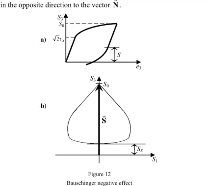
Abstract: The paper is concerned with the generalization of the synthetic theory to the modeling of both plastic and creep deformation. Non-classical problems such as creep delay, the Bauschinger negative effect and reverse creep have been analytically described;

the calculated results show satisfactory agreement with experiments. These problems cannot be modeled in terms of classical creep/plasticity theories. The main peculiarity of the generalized synthetic theory consists in the fact that the macro-deformation is highly associated with processes occurring on the micro-level of material.

Keywords: plastic deformation; primary creep; steady-state creep; the Bauschinger negative effect; creep delay; reverse creep

1 Introduction

The work presented herein regards the generalization of the synthetic theory of plastic deformation [18] to the modeling of not only plastic, but also creep (both primary and steady-state) deformation. This theory, which is concerned with small strains of work-hardening metals, incorporates (synthesizes) the Budiansky slip concept and the plastic flow theory developed by Sanders.

The key points of the generalized synthetic theory are:

I It is of both mathematical and physical nature. As a mathematical (formal) theory, the synthetic theory is in full agreement with the basic laws and principles of plasticity, such as Drucker’s postulate, the law of the deviator proportionality, the isotropy postulate, etc. [18]. As a physical model, the synthetic theory allows for real processes occurring at the micro-level of material during loading, and the macro-behavior of material is fully governed by these processes. Therefore, the synthetic theory is a two-level theory.

II Independently of the type of deformation (creep or plastic) to be modeled, a single notion, irreversible (permanent) deformation is introduced, i.e. the

deformation is not split into “instantaneous” plastic and viscous parts [17]. The manifestation of the plastic or viscous component and their interrelations depend on the concrete loading/temperature-regime. The correctness to use the notion of irreversible deformation follows from the similarity of the mechanism of time- dependent and plastic deformation. Indeed, this mechanism is slips of the parts of crystal grains relative to each other. These slips are induced mainly by the motions of dislocations which, in turn, are induced/accompanied by other micro-structural imperfections (defects) of the crystalline lattice (vacancies, interstitial atoms, etc.).

Undoubtedly, the driving forces and concrete configurations of the defects are different under different conditions. Nevertheless, despite the variety of processes occurring in a body subjected to different loading regimes, numerous experiments systematically record the arising of dislocation gliding for any type of inelastic straining. Other facts justifying the similarity of the nature of plastic and time- dependent deformation are (i) hydrostatic stress does not affect creep deformation;

(ii) the axes of principal stress and creep strain rate coincide; (iii) no volume change occurs during creep [3]. These observations are the same as those for plastic deformation [6, 7].

III Following the tendency of unified approaches to the determination of irreversible deformation [4, 5], the system of constitutive equations that governs the whole spectrum of inelastic deformation has been worked out. In terms of generalized synthetic theory, the universality of this system is based on:

(i) a single equation provides the relation between a) micro-irreversible deformation, b) defects of crystalline structure inducing this deformation and c) time. Further, the procedure of the transition from micro- to macro-level is also uniformed: the sum of irreversible micro-strains determines the magnitude of macro-strain.

ii) the hardening rule is set in such a way that the transformation of loading surface obeys a unique rule. In addition, the kinetics of the loading surface transformation is not set a priori but is fully determined by the loading regime.

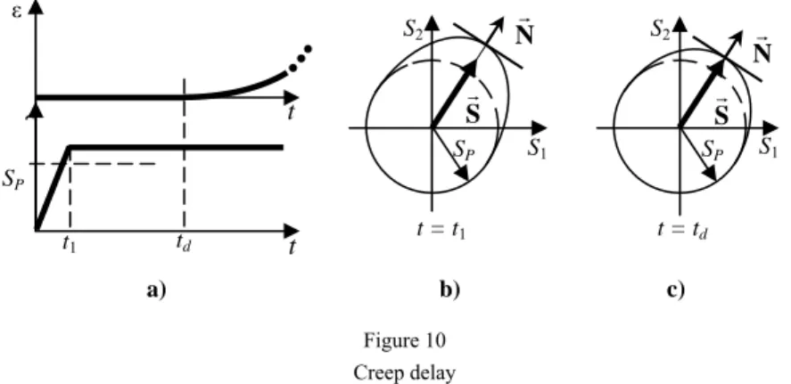
The objectives of this papers are to demonstrate how, by utilizing the uniformed method, the generalized synthetic theory is capable of embracing both plastic and creep deformation. In addition, some non-classical problems such as creep delay, the Bauschinger negative effect and reverse creep [12] are considered. The investigation of reverse creep is of great importance due to the fact that this phenomenon contradicts the hypothesis of creep potential [3, 13]. The advantages of synthetic theories above classical theories of creep and plasticity are considered.

2 Fundamentals of the Synthetic Theory of Plastic Deformation

The synthetic theory is based on the Budiansky slip concept [2] and the plastic flow theory developed by Sanders [19]. Below, the basic principles of the synthetic theory [18] are briefly reviewed.

A) The establishment of strain-stress relationships takes place in the Ilyushin stress deviatoric space, S⁵, [8]. A load is presented by stress-deviator vector, S, whose components are defined as

Sxx

S₁= 32 , S₂=S_xx 2+ 2S_yy, S₃= 2S_xz, Sxy

S₄ = 2 , S₅= 2S_yz, (2.1)

where S_ij (i, j = x, y, z) are the stress-deviator tensor components; S =3 2J₂, where J2 is the second invariant of stress deviator tensor [7]. Further throughout we will consider the cases when S∈S³ (S₄ =S₅ =0).

B) Yield criterion and yield surface. One of the key points consists in the construction of planes tangential to the yield surface in S⁵ instead of the yield surface itself. The inner-envelope of tangent planes constitutes the yield surface.

By making use of this method, a new yield criterion is introduced, which coincides with neither the Tresca nor the von-Mises yield criterion in S⁵. At the same time, the new criterion is reduced to the von-Mises yield criterion in S³ meaning that the trace of the five-dimensional yield surface takes the form of a sphere in S³ (S₄=S₅=0):

2 32 22

12 S S 2 _S

S + + = τ , (2.2)

where τ_S is the yield limit of a material in pure shear.

C) Loading surface. Following Sanders [19], the stress deviator vector shifts planes tangential to the yield surface on its endpoint during loading. The movements of the planes located on the endpoint of stress deviator vector are translational, i.e. without a change in their orientations. Those planes which are not on the endpoint of the stress deviator vector remain unmovable. Despite the fact the S∈S³, the displacements of planes tangential to the five-dimensional yield surface must be considered. On the other hand, the positions of these planes can be set by their traces in S³. As a result, any plane in S³ (either tangential to the sphere (2.2) or locating beyond this sphere) is the trace of the plane tangential to the five-dimensional yield surface [18].

Figure 1

Yield and loading surface in terms of synthetic theory

The loading surface constructed as the inner-envelope of the tangent planes takes the shape fully determined by the current positions of the planes. Therefore, the behavior of the loading surface is not prescribed a priori, but is fully determined by the hodograph of the stress deviator vector.

For simplicity, let S1-S2 coordinate-plane play the role of S³. Then, Fig. 1a illustrates the yield surface (2.2) (circle) in the virgin state of the material. The planes (lines) tangential both to the five-dimensional yield surface and to its trace in S³ are shown as solid lines. The lines filling up the S1-S3 plane beyond the

S1

S2

S1

S S2

a)

b)

circle (the traces of the planes tangential to only the five-dimensional yield surface) are shown as dotted lines.

Fig. 1b shows loading surface due to the action of vector S∈S³ which shifts a set of planes. It is easy to see that the corner point arises on the loading surface at the endpoint of S (loading point). This fact is of great importance for the description of the peculiarities of plastic straining at non-smooth (orthogonal) loading trajectories [18] where any theory with regular loading surface has proved to be unsuitable.

The condition that the tangent plane is located on the end-point of the stress deviator vector can be expressed as

N S⋅

N =

H , (2.3)

where H_N is the distance between the origin of coordinates and the tangent plane in S⁵; N is the unit vector normal to the tangent plane, which defines the orientation of the plane. If the plane is not reached by S, H_N >S⋅N. The distance to plane in S⁵ can be expressed through that to its trace in S³,h_m, as

λ

= _mcos

N h

H , (2.4)

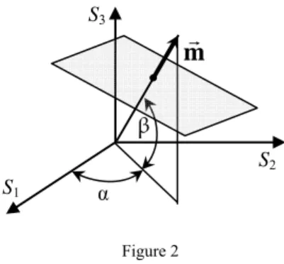
where index m indicates the unit vector, m, normal to the tangent plane in S³:

(

cos^αcos^β,sin^αcos^β,sin^β

)

m , (2.5)

In expression (2.4), λ is the angle between the vectors m and N. The angles α and β are shown in Fig. 2.

Figure 2

Orientation of normal vector

m

In addition, the N and m vector components are related to each other as [18]

λ

= _k cos

k m

N , k=1,2,3 S1

S2

S3

m

 β

λ β α

=cos cos cos

N1 , N₂=sinαcosβcosλ, N₃=sinβcosλ., (2.6) Therefore, expressions (2.3) and (2.6) give that

(

+ +

)

λ

= λ

⋅

= cos S₁m₁ S₂m₂ S₃m₃ cos

H_N S m , S∈S³. (2.7)

As follows from formulae (2.4) and (2.6), if λ=0, then H_N =h_m and N_k =m_k (k=1,2,3). This holds true only for the planes which are tangential both to the five-dimensional yield surface and to its trace in S³. It is these planes with λ=0 that govern the transformation of the loading surface in S³ [18].

D) Plastic strain vector components. Similarly to the Batdorf-Budiansky slip concept, the synthetic theory is of a two-level nature. Each tangent plane represents an appropriate slip system at a point in a body (microlevel, see Fig. 3), and the plane motion symbolizes an elementary process of plastic deformation within this slip system.

Figure 3

Two levels of the determination of deformation

To define an average, continuous measure of plastic slip within one slip system, we introduce a scalar magnitude, plastic strain intensity (ϕ_N), is proposed as

S S

N

N H

rϕ = − 2τ =S⋅N− 2τ . (2.8)

Formula (2.8) holds true for the planes displaced by the stress deviator vector, i.e.

if H_N =S⋅N. If H_N >S⋅N, ϕ_N is set to be zero. An incremental plastic strain-vector,de^S, (micro plastic deformation on the lower(micro)-level) is assumed to be in the direction of the outer normal to the plane and determined as

dV

de^S =ϕ_NN . (2.9)

Macrolevel (a point in a body)

Microlevel (slip system)

In expression (2.9), dV is an elementary volume constituted of the elementary set of planes in S³ that covered an elementary distance due to an infinitesimal increase in the stress vector [1]:

λ β α β

= d d d

dV cos . (2.10)

The total (macro) plastic strain-vector at a point in a body, e^S, is determined as the sum (three-folded integral) of the micro plastic strains ‘produced’ by movable planes:

∫

^ϕ

=

V

S NNdV

e or ⁼

∫

^ϕ

V

S NNdV

e (2.11)

The strain vector components relate to the strain-deviator tensor components e_ij (i, j = x, y, z) as [8]

exx

e₁= 32 , e₂=e_xx 2+ 2e_yy, e₃= 2e_xz, exy

e₄= 2 , e₅= 2e_yz. (2.12)

By using equations (2.6) and (2.10), equation (2.11) becomes

∫∫∫

α β λ

λ β α β λ ϕ

= m d d d

e_k^S _{N k}cos cos or

α β λ

∫∫∫

λ β α β λ ϕ

= m d d d

e_k^S _{N k} cos cos , k=1,2,3 (2.13)

The integration in (2.13) must be taken over planes shifted by the stress deviator vector.

3 The Generalization of the Synthetic Theory

To extend the boundaries of the applicability of the synthetic theory, the following is proposed.

I) To reflect the well-known fact that the defects of the crystal structure of metals are the carriers of irreversible deformation, a new notion, defect intensity (ψ_N), is introduced. ψ_N represents an average continuous measure of the defects (dislocations, vacancies, etc.) generated by irreversible deformation within one slip system.

II) To model the influence of loading rate upon irreversible straining, a new function of time and loading rate, the so called integral of non-homogeneity (I_N), is introduced. By considering the physical nature of irreversible deforming, the formula for I_N will be strictly derived in 3.1.2.

III) Instead of (2.8), the defect intensity is related to H_N and I_N:

P N

P N

N

N =H −I − τ = ⋅ −I − τ

ψ 2 S N 2 , (3.1)

where τ_P is the creep limit of material in pure shear. In terms of the generalized synthetic theory, the yield and creep limits are related to each other by equation derived further (see 4.1)). The establishment of a relationship between ψ_N and HN is fully logical, because the distance H_N characterizes the degree of work- hardening. Indeed, the greater the plane distance, the greater a stress deviator vector is needed to reach the plane, i.e. to induce irreversible strain.

IV) To establish a relationship between irreversible deformation, defects and time (t), the following equation is proposed

dt K rd

dψ_N = ϕ_N − ψ_N , (3.2)

where, r is the model constants and K is a function of homological temperature, Θ, and S (see 5). The units of quantities in (3.2) are

[ ]

ψ_N =Pa,

[ ]

ϕ_N =1,

[ ]

r =Pa and

[ ]

K =sec⁻¹.

In what follows, the parameter of non-homogeneity and the detailed analysis of the proposed generalizations are considered.

3.1 The Integral of Non-Homogeneity

3.1.1 Local Micro-Stresses and the Physics of Primary Creep

As is well known, plastic deformation is accompanied by the formation of dislocation pile-ups, tangles of dislocations, unmovable jogs, grains boundaries, etc (the nucleation of dislocations is also observed at elastic deformation). These defect-formations, being of strongly local character, raise an uneven stress/strain distribution through the microstructure of metal that, in turn, leads to considerable distortions of the crystal lattice where the strain energy is mainly stored.

The considerable non-homogeneity and concentration of micro-strains/stresses of the second and third kind were observed in experiments performed on specimens of pure copper, iron and titanium [9]. The experiments show that both stresses and strains are distributed non-homogeneously within grains (under both elastic and plastic loading). In addition, if the strain is greater than its average value through

the grain, then the stress inducing this strain is smaller than average stress and vise verse. At the same time, the total over- and under-loading is equal to zero.

The non-homogeneous stress distribution makes the metal structure more unstable than in an annealed state. Once favorable conditions arise (for example, if the stress stops increasing), the relaxation of crystal lattice distortions is observed. It is the difference between the local and average stresses that is the driving force for the relaxation that occurs mainly due to spontaneous slips in grains induced by the movements of dislocation. Indeed, under thermal fluctuations, locked and tangled dislocations and the obstructions in their way themselves become progressively movable, thereby promoting the development of deformation. Therefore, the time dependent relaxation of the crystal lattice distortions governs the progress of the primary creep deformation.

The local stresses arising around the lattice distortions we will call local microstresses. These stresses display the following properties: 1) they, being directly correlated with dislocation density, make the material stronger; 2) the greater the loading rate, the greater the local stresses; 3) they are unstable: as soon as favorable conditions arise, they decrease with time. It must be noted that the local microstress relaxation is also observed during slow loading.

Therefore, on the one hand, the local microstresses cause the “rate-hardening” of the material during active loading but, on the other hand, they can relax resulting in the softening of the material. Time-dependent macro-deformation is the result of the concurring processes of the hardening and softening.

3.1.2 The Integral of Non-Homogeneity as the Mathematical Measure of Local Stresses

To establish a relation between the microstress non-homogeneity and elastic strain energy, consider an elementary volume of body (treated as point) consisting of a large number of microparticles. Let σ_kq⁰ denote the average stress deviator tensor components (macrostress) acting at the given point. The microstress non- homogeneity can be expressed through the stress deviator tensor components acting in each microparticle, σ_kq, as

0 ' kq kq kq =σ +σ

σ , (3.3)

where σ_kq' are random quantities expressing the over/under-loading in each particle. We set the reaction of σ_kq' on the change in the average stress as

' _{ijkq ij}0

kq C d

dσ = σ , (3.4)

where C_ijkl are random numbers that vary from particle to particle, which are assumed to be independent from σ_ij⁰. Let us suppose that all random numbers Cijkl have an identical distribution function, F, and are independent of each other.

Since dσ_ij⁰ are macroscopic (average) stress components, the mathematical expectation of parameters C_ijkl is

( )

=0

∫

∞

∞

−

ijkl ijkl ijklFC dC

C Σ (3.5)

Formula (3.5) means that the total over/under-loading with respect to the average stress is equal to zero. In addition,

( )

⁼¹

∫

∞

∞

−

ijkl ijkl dC C

F Σ, (3.6)

As was pointed out earlier, the local stresses are unstable and can relax with time.

The equation governing their time-dependent behavior is proposed as dt

p d C

dσ_ij'= _ijpq σ_pq⁰ − σ_ij' . (3.7)

The first item on the right side in the above formula characterizes the rise of σ_ij' given by (3.4); term −pσ_ij'dt gives the time-dependent decrease of microstresses, which is taken to be proportional to σ_ij'. The solution of the differential equation (3.7) for σ_ij' is

( )

t I C_{ijkq kq} ij =

σ ' , ^Ikq

( )

^{t =}

∫

^{t dσ}_ds^kq

(

^{− p}

(

^t−s

) )

^ds

0 0

exp . (3.8)

Now, expression (3.3) becomes

( )

t I C_{ijkq kq}

ij ij =σ +

σ ⁰ . (3.9)

As is well known, elastic strain energy can be expressed as

( ) ( ) ( ) ( )

[

^{2 2 2 6 2 2 2}

]

12 1

zx yz xy xx

zz zz

yy yy

G xz

U= σ −σ + σ −σ + σ −σ + τ +τ +τ , (3.10) where G is the elastic shear modulus. By substituting stresses σ_ij from (3.9) into (3.10), we obtain

( ) ( )

( )

( ) ( ) ( )

⎭⎬

⎥⎦⎫

⎢⎣ ⎤

⎡τ + +τ + +τ +

+

+

− σ

− +

σ +

+

− σ

− +

⎩ σ

⎨⎧σ + −σ − +

=

0 2 0 2

0 2

0 2 0

0 2 2 0

0 0

6 12

1

kq xzkq xz kq yzkq yz kq xykq xy

kq xxkq xx kq zzkq zz

kq zzkq zz kq yykq yy kq yykq yy kq xxkq xx

I C I

C I

C

I C I

C

I C I

C I

C I

G C U

(3.11)

The mean value of U is determined by the following relation

(

^C_xxxx

)

^F

(

^C_xzxz

)

^dC_xxxx ^dC_xzxz

UF

U … … …

36

∫

∫

^∞

∞

−

∞

∞

−

= . (3.12)

U can be decomposed in two parts:

2

1 J

J

U = + , (3.13)

( ) ( )

₀

0 36

1 U F C F C dC dC U

J =

∫

^∞

∫

_{xxxx xzxz xxxx xzxz} =

∞

−

∞

∞

−

…

…

… , (3.14)

( ) ^{( ) ( )}

( ) ( ) ^{( )}

( )

^…

( )

^…

( )

^{… …}

…

…

…

…

…

…

…

+

⋅ σ

+

+

⋅

=

= +

σ +

=

∫

∫

∫

∫

∫

∫

∫

∫

∞

∞

−

∞

∞

−

∞

∞

−

∞

∞

−

∞

∞

−

∞

∞

−

∞

∞

−

∞

∞

−

xzxz xxxy xzxz xxxy

xxxx xxxx xxxx xx xx

xzxz xxxy xzxz xxxy

xxxx xxxx xxxx xx

xzxz xxxx xzxz xxxx

xx xx xxxx xx xxxx

dC dC C F C F dC

C F C GI

dC dC C F C F dC

C F C GI

dC dC C F C F I

C I G C

J

35 0

35 2

2

0 2

2

36 2

6 1

12 1 12 2 1

(3.15)

where U₀ is the strain energy for the case of homogeneous stress distribution determined by formula (3.10) at σ_ij =σ_ij⁰. In arriving at the result (3.14), expression (3.6) has been taken into account. In order to evaluate integral J₂, it is enough to investigate its first two terms. Indeed, formula (3.5) implies that all the integrals in (3.15) containing C_ijkl are equal to zero. The integrals containing

2

Cijkl give the variance of random numbers C_ijkl, B₁:

( )

1

2 F C dC B

C_{ijkl ijkl ijkl} =

∫

∞

∞

−

Σ. (3.16) As a consequence,

(

^{2 2 2 2 2 2}

)

2 2 1 2 2 2

zx yz xy zz yy

xx I I I I I

G I

J = B + + + + + .

Finally, expression (3.13) is

(

^{2 2 2 2 2 2}

)

0 2 1 2 2 2

zx yz xy zz yy

xx I I I I I

G I U B

U = + + + + + + . (3.17)

By subtracting from the right-hand side in (3.17) the expression

( )

²

1 3

2B G I_xx+I_yy+I_zz , which is equal to zero due to σ⁰_x+σ⁰_y +σ⁰_z =0, we obtain

( ) ( ) ( ) ( )

[

^{2 2 2 2 2 2}

]

1 0 3 6 2

zx yz xy xx

zz zz

yy yy

xx I I I I I I I I

G I B

U U

+ + +

− +

− +

− +

+

=

. (3.18)

Substituting I_ij from (3.8) into (3.18) and converting the variables σ_ij to the stress vector components S_n by formula (2.1), the expression for the mathematical expectation of elastic strain energy is obtained as

( )

( )

5 2

1 0

0 1 exp

3

2

∑ ∫

= ⎥⎥

⎦

⎤

⎢⎢

⎣

⎡

−

− +

=

n t

n pt s ds

ds dS G

U B

U (3.19)

The value of U is seen to consist of two parts; the term U₀ corresponds to homogeneous stress distribution and the second term characterizes the time- dependent deviation of stresses from their average value. If a body is ideally homogeneous, the distribution functions of random numbers C_ijkl degenerate in the Dirac delta-function and, according to (3.16), we obtain B₁=0. As seen from formula (3.19), U depends not only on the rate of stress vector components S_n at a given instant, but on its values for the all history of loading as well. For the case S_n =const,

( )

( )

2

0

0 1 exp

3 2

⎥⎥

⎦

⎤

⎢⎢

⎣

⎡

−

− +

= G ^SnSn

∫

^{t pt s ds}

U B

U . (3.20)

Since S_nS_n =S² (S denotes the length of stress vector),

( )

( )

2

0

0 1 exp

3 2

⎥⎥

⎦

⎤

⎢⎢

⎣

⎡

−

− +

=

∫

^t ds ^{pt s ds}

dS G U B

U . (3.21)

In the case that the stress deviator vector has only one non-zero component, expressions (3.19) and (3.21) are identical. We take the square root in the right- hand side in relation (3.21) to be the scalar measure of micro-non-homogeneity:

( )

( )

∫

^{− −}

=

t

ds s t ds p

B dS I

0

exp , const

G B= B =

3 2 ₁

. (3.22) We will term I as the integral (parameter) of non-homogeneity. To work with the

integral of non-homogeneity on the microlevel of material, we replace S in (3.22) by scalar product S⋅N. This replacement reflects the fact that the driving force of plastic flow within a slip system is not the whole macro-stress vector S but only its projection S⋅N (resolved stress). Thus, finally, the characteristic of local micro-stresses has the form

( )

( )

∫

^{⋅ − −}

=

t

N pt s ds

ds B d I

0

exp

S N . (3.23)

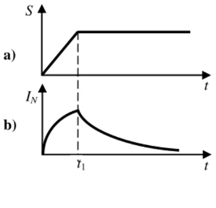
In contrast to (3.22), the adopted integral (3.23) depends on angles α, β, and λ thereby allowing for the orientation of tangent planes in the Ilyushin subspace S³. Let us analyze the integral of non-homogeneity for the loading regime shown in Fig. 4 (v=dS dt=const). On the first portion of the loading, formula (3.23) gives

( ) ( ) ( ( ) ) ( ) _{[ (}

_pt

_{) ]}

p ds B s t p B

t I

t

N ⋅ − −

=

−

−

⋅

=

∫

^{exp 1 exp}

0

N N v

v , t∈

[ ]

0,t₁ . (3.24)

As seen from (3.24), I_N

( )

t grows from the very beginning of loading. If we take the loading rate v=S/t to be infinitely large, we can approximate the function

(

^{− pS v}

)

exp in (3.24) by the Tailor series, which results in the following relation

( )

^S⋅N

=B

I_N as v→∞. (3.25)

For the range t>t₁ when v=0, let us split the range of integration in formula (3.23) into two parts,

[ ]

0,t₁ and

[

^t₁,^t

)

:

( ) ( ) ( ( ) ) ( ) _{[ ( )}

_pt

_{] (}

_pt

₎

p ds B s t p B

t I

t

N = ⋅

∫

^1exp− − = ⋅ ^{exp 1} −^1exp−

0

N N v

v , t≥t₁. (3.26)

From (3.24) and (3.26) the following properties of the integral of non- homogeneity can be indicated: (i) during loading, it grows proportionally to the loading rate; (ii) it decreases under constant loading. Therefore, the time- dependent behavior of the integral of non-homogeneity correlates with that of local microstresses.

The condition I_N =0 symbolizes the end of transformations occurring in the crystal lattice under primer creep and transition to the steady-state stage of creep.

Figure 4 IN-t diagram

Intermediate discussion. The sum of the two quantities in equation (3.1),

P N

N+I = ⋅ − τ

ψ S N 2 , characterizes the straining state of the material and determines the stress to induce irreversible deformation. The parameters ψ_N and

IN have a common trait; they can relax in time (see (3.2), and (3.26)). On the other hand, there is an essential difference between these quantities: ψ_N expresses the number of defects that produce irreversible deformation, whereas

IN characterizes the loading-rate-dependent development of these defects. The integral I_N behaves in a different way depending on loading regime: a) under loading, I_N symbolizes the load-rate strengthening of material; b) under constant stress, I_N drops expressing the lattice distortion relaxation that results in time- dependent, progressive deformation. The behavior of ψ_N and I_N is governed by different equations; I_N depends on loading-rate-history, formula (3.23), whereas

ψN is related to irreversible deformation by (3.2).

t IN t

t1

a)

b) S

3.2 System of Constitutive Equations

Formulae (3.1), (3.23), (3.2) and (2.13) constitute the base of the generalized synthetic theory:

P N

N

N =H −I − τ

ψ 2 , (A)

( )

( )

∫

^{⋅ − −}

=

t

N pt s ds

ds B d I

0

exp S N

, (B)

dt K rd

dψ_N = ϕ_N − ψ_N , (C)

α β λ

∫∫∫

λ β α β λ ϕ

= m d d d

eⁱ_{k N k} cos cos or

∫∫∫

α β λ

λ β α β λ ϕ

= m d d d

e_kⁱ _{N k} cos cos , k=1,2,3

(D)

The procedure of the calculation of irreversible strain vector components (eⁱ_k) is the following, (i) at a given stress deviator vector and loading rate, the defect intensity is determined by (A) and (B), (ii) the strain intensity can be found by (C) and, finally, (iii) formula (D) gives the values of strain(rate) vector components.

Expression (C) is one of the most important in terms of the generalized synthetic theory. It reflects the well-known fact that the defect intensity dψ_N grows with the increase in deformation (rdϕ_N ) and simultaneously decreases (relaxes) with time (−Kψ_Ndt ). Owing to (C), one does not need to split a deformation into its “instantaneous” (plastic) and viscous parts; both of them develop simultaneously. The degree of this development depends on concrete loading- and temperature-regimes. That is why, further throughout, we will use a single notion, irreversible deformation, by which we mean the deformation progressing with time (independently of whether we consider very short-termed loadings at plastic deformations or loadings lasting several hours or days as in creep tests).

The (A)-(D) system governs all types of irreversible deformation for any state of stresses and loading regimes.

Regard must be paid to the integration limits in formula (D). When founding the boundary values of angles α, β and λ, one must follow a single rule – only tangent planes which are on the endpoint of the stress deviator tensor produce irreversible strains. Since the plane distances are related to ψ_N , the limits of integration in (D) are determined from the conditions ψ_N = 0,

0≤λ≤λ1,

( ) ( )

N P

−I

⋅

= τ β α λ

m S , 2

cos ₁ . (3.27)

The condition λ₁=0 gives the equation for the boundary values of angles α and β:

P

IN = τ

−

⋅m 2

S . (3.28)

4 Irreversible Deformation in Terms of the Generalized Synthetic Theory

4.1 Creep-Yield Limit Relation

Consider the case of arbitrary stress state, and assume that the loading rate is infinitely small so that the parameter of non-homogeneity tends to zero. If an irreversible deformation does not occur, ψ_N =0, formula (A) gives that the tangential planes in S³ (λ=0) are equidistant from the origin of coordinates:

( )

_N

( )

_P

m H

h α,β = α,β,λ=0 = 2τ . (4.1)

The above formula implies that the creep surface (creep locus in S³ setting the condition for the onset of first plastic flow at infinitesimal loading rate), being constructed as the inner-envelope of tangential planes, takes the form of the sphere of radius 2τ_P:

2 32 22

12 S S SP

S + + = , S_P = 2τ_P. (4.2)

For the case of pure shear, expression (2.1) gives S₃= 2τ_xz and S₁=S₂=0 meaning that the stress vector S

(

0,0,S3

)

acts along S3-axis. Let τ_P denote the value of shear stress when vector S

(

0,0, 2τP

)

reaches the first tangential plane on the sphere (4.2). Since this plane is perpendicular to S3-axis (β=π 2 and

=0

λ ), formulae (2.5) and (2.7) give H_N = 2τ_P. Therefore, τ_P expresses the creep limit of metal in pure shear.

Now, our goal is to establish the relation between τ_S and τ_P. It is worth starting with the case of pure shear. Let the loading be of constant rate,

const S S

v= ₃= = , S = S. Then expression (3.23) becomes

( )

( )

∫

^{− −}

λ β

=

t

N Bv pt s ds

I

0

exp cos

sin . (4.3)

Until the stress vector reaches the tangential planes, ψ_N =0, formula (A) takes the form

P N

N I S

H = + . (4.4)

By integrating in (4.3) and inserting the result of the integration in (4.4), we obtain

( )

[ ]

_P

N pt S

p

H =Bv 1−exp− sinβcosλ+ , t∈

[ ]

0,t1 in Fig. 4a. (4.5) As seen from (4.5), the plane distances grow due to the increase in I_N. This means that formula (4.5) describes the movements of planes in the direction away from the origin of coordinate. Since these movements are not caused by the

“pushing” action of stress deviator vector, they do not cause irreversible strain.

The inner envelope of the planes with distances from (4.5) is shown in Fig. 5a (only tangent planes with λ=0 are shown). As seen, the action of the integral of non-homogeneity does not result in the formation of a corner point.

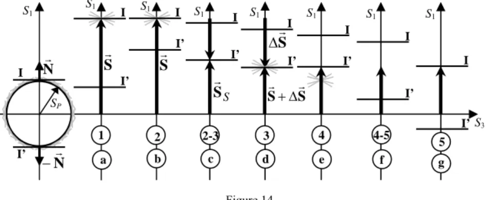
Figure 5

The transformation of yield (a and b) and loading (c) surface

Let S_S denote the length of the stress deviator vector which at time t_S (t_S∈

[ ]

0,t1 ) reaches the first plane (β=π 2 and λ=0), i.e. the plastic flow starts developing (Fig. 5b). For this plane, formula (2.7) gives H_N =S_S. The replacement of H_N by S_S in (4.5) leads to the equation for S_S:

( )

(

_S

)

_P

S pt S

p

S = Bv 1−exp− + , S_S =vt_S (4.6)

S₁ S1

S₃ S₃

τP 2

SS

= S

β1 β1

( tS)

t∈0, t=tS t=t₁

c)

a) b) _S<SS

N N

S1

S₃

SS

>

S

The plot of S_S as the function of v constructed on the base of (4.6) is shown in Fig. 6. As follows from Eq. (4.6), curve ^S_S ^=S_S

( )

^S_P has a horizontal asymptote, which is at a distance of ^S_P

(

1−^B

)

from the abscissa that corresponds to the case of an infinitely large loading rate.

For S >S_S, the stress deviator vector translates some set of plane (Fig. 5c), and angle β₁ gives the boundary planes on the endpoint of S.

Further, let us find the yield limit for an arbitrary proportional loading with a constant loading rate. Now, expression (3.23) is

( )

[ ]

∫

^⎜_⎝^{⎛ α β+ α β+ β⎟}_⎠^{⎞ − −}

×

× λ

=

t N

ds s t ds p

dS ds

dS ds

dS B I

0

3 2

1cos cos sin cos sin exp

cos

. (4.7)

Figure 6

Yield limit vs loading rate plot

In the direction of the action of the stress deviator vector whose orientation is given by angles α₀ and β₀, relations

(

2 2²

)

¹²

1 1

cosα0=S ⋅ S +S ⁻ and

0 1

sinβ =S₃⋅S⁻ hold true and formula (4.7) yields the form

( )

[ ]

∫

^{− −}

λ

=

t i i

N pt s ds

ds dS S B S

I

0

0 cos exp . (4.8)

Since S can be expressed as

dt dS S S dt

S =dS = ^{i i} , Eq. (4.8) gives

( )

[ ]

∫

^{− −}

λ

=

t

N pt s ds

ds B dS

I

0

0 cos exp . (4.9)

The integral I_N0 is identical to that from (4.3) at β=π 2 meaning that formula (4.6) is applicable to the determination of yield limit via the creep limit for an arbitrary state of stress.

v SS

SP

B S_P

− 1

Summarizing, formula (4.6) is of great importance due to the fact that it allows working with only one material constant, creep limit. In contrast to classical theories of plastic/creep deformation that use separately yield limit or creep limit depending on the problem to be solved, the generalized synthetic model is constructed in such a way that the creep limit plays the role of the material constant, while the yield limit is a function of loading rate.

4.2 The Modeling of Irreversible Deformation

Consider the case of proportional loading when the loading trajectory is a straight line in S³. Further, let the plot of ^S

( )

^t have the form as in Fig. 4. Since the synthetic theory provides the fulfillment of the law of the deviator proportionality [14-16, 18], the formulae obtained for the case of, e.g., pure shear are fully applicable (up to constants) to arbitrary rectilinear loading path in S³.

For the case of pure shear, expressions (A), (2.5) and (2.7) give the defect intensity as

[ ]

_{P P}

N S

S a I

S ⎟

⎠

⎜ ⎞

⎝⎛ −Ω

=

− λ β

−

=

ψ ₃ sin cos 1 , S₃>S_S, (4.10)

λ β

= λ

=

Ω m₃cos sin cos , (4.11)

I S a S^P

= −

3

. (4.12) In formulae (4.10) and (4.12)

( )

[

^{pt s}

]

^ds

ds B dS I

t

−

−

=

∫

^exp

0

3 , (4.13)

( )

[

1

]

1 1 1 exp pt

p I Bv

It₌t ≡ = − − , v=S₃=S=const, (4.13a)

[ ( )

^pt

] ( )

^pt

p I Bv

It_>t ≡ ₂= exp ₁ −1exp−

1 . (4.13b)

According to (3.27) and (3.28), the defect intensity in expression (4.10) is positive for

π

≤ α

≤ 2

0 , β₁≤β≤π 2, 0≤λ≤λ₁,

β

= β λ sin

cos ₁ sin ¹ , sinβ₁=a (4.14) The loading surface at t=t₁ is shown in Fig. 5c or 7a.

The defect intensity increment is expressed from (4.10) as

(

−

)

Ω

=

ψ dS dI

d _{N 3} . (4.15)

Beyond the angles-diapason given by (4.14), we have ψ_N =dψ_N =0 and

=0 ϕ

=

ϕ_N d _N .

Figure 7

Kinetics of loading surface at creep

Consider the transformation of the loading surface for t>t₁ when S₃=0. For the tangent planes that are beyond the diapason (4.14), formula (A) at ψ_N =0 gives

λ β +

=S I₂sin cos

H_{N P} . (4.16)

Because of the descending character of I₂, we infer that H_N decreases for t>t₁ meaning that planes that are not on the endpoint of the stress deviator vector at

t1

t= start to move towards the origin of the coordinates. These movements result in the greater number of planes becoming located at the endpoint of the stress deviator vector. This situation is illustrated by Fig. 7b from which it is seen that the boundary angle β₁ determined by (4.14) and (4.13b) decreases with time. As integral I₂ tends to zero, formula (4.16) gives H_N =S_P meaning that the planes stop moving and the boundary angle β₁ takes its minimal value (Fig. 7c).

Further, formula (B) gives the strain intensity as

( )

^dt

KS a dI

dS dt K d

rd _{N N N P} ⎟

⎠

⎜ ⎞

⎝

⎛Ω− +

Ω

−

= ψ + ψ

=

ϕ ₃ 1 . (4.17)

Finally, formulae (C) gives the increment in irreversible-strain-vector-component, e₃i

Δ , as S3

S1

S3

N

N N N

β1 β₁

β1

β1

β1 β1

N

N

t1

t>

>0

IN I_N =0

>0 IN

a) b) c)

t1

t=

t1

t>

S3

τP 2

∫

∫

∫

^{π λ}

β π

λ λ ϕ Δ β β α

= Δ

1

0 2

1 2

0

3 sin2 cos

2

1 d d d

eⁱ r _N , (4.18)

where Δϕ_N is given by (4.17). In formula (4.18), the symbol Δ stands for the time-dependent increment of Δe₃ⁱ and Δϕ_N. By integrating over α, β and λ in (4.18), we obtain

( ) ( )

[

^{a K a t}

]

a

eⁱ = ΔΦ + Φ Δ

Δ _{3 0} , (4.19)

where

const a πτr ^p =

= 3 2

0 ,

( )

a a a

a a a a

2 2

2 1 1

ln 1

arccos −2 − + + −

=

Φ , Φ

( )

1 =0. (4.20)

The analysis of (4.20) shows that the function Φ is in inverse proportion with its argument a, Fig. 8.

Figure 8 Φ(a) function

By integrating over time in (4.19), we obtain the formula for the irreversible strain component in pure shear as:

( ) ( )

⎥⎥

⎥

⎦

⎤

⎢⎢

⎢

⎣

⎡

Φ + Φ

=

∫

^t

tS

i a a K adt

e_{3 0} . (4.21)

To evaluate the integral (4.21), one needs to know the function K

(

S₃

( )

t ,Θ

)

. This question will be considered in detail in 5.

Following the law of deviator proportionality [14], formula (4.21) can be rewritten for the case of an arbitrary stress state as

( ) ( )

S dt S a K a a

e ^k

t

tS i

k ⎥⎥⎥

⎦

⎤

⎢⎢

⎢

⎣

⎡

Φ + Φ

= ⁰

∫

^{k=1,2,3 (4.22)}

where, instead of (4.12),

Φ

1 a

I S a S^P

= − , (4.23)

and I is calculated by (4.13a) and (4.13b) where v=S=const.

Formula (4.22) is of a general character; it is applicable to the modeling of any type of deformation, both plastic and unsteady/steady-state creep. At t=t₁, we obtain the plastic strain vector components; at t>t₁ we get the total, plastic and creep, strain components.

4.3 The Analysis of the System of Constitutive Equations.

Partial Cases

1) Consider the case of steady-state creep when dS=0 and I_N =0. It is clear that expression (4.15) gives dψ_N =0, i.e. the defect intensity (density) does not change during the steady state creep, reflecting the well-known fact that the steady-state creep deformation develops under the equilibrium between the processes of hardening and softening. Therefore, formula (C) gives the constant strain intensity rate:

const K

rϕ_N = ψ_N = , K

(

S,Θ

)

=const. (4.24)

Another consequence from conditions dS=0 and I_N =0 is a=S_P S=const and Φ

( )

a =const (see (4.20) and (4.23)). According to (4.22), the steady-state creep strain(rate) components, e_k^P, can be written as

( ) ( )

t

S a S K S a a S a

e_k^P = ₀Φ ^k + ₀ Φ ^k or

( )

const S

a S K a

e_k^P = ₀ Φ ^k = (4.25)

where a₀Φ

( ) (

a ⋅ S_k S

)

is the value of strain at the end of primary creep. Formula (A) shows that the plane distances do not change with time, meaning that the steady state creep deformation is “produced” by the set of motionless planes which are located on the endpoint of the stress deviator stress (Fig. 7c). Since function K appears in the formula for steady-state creep rate, we can infer that it takes very small values, and the manifestation of the second term in (4.22) becomes material only under long-termed loadings. At the same time, it is important to emphasize that the role of the time integral in (4.22) grows with the increase in the duration of loading especially at elevated temperatures.

2) On the basis of the above, we can neglect the second term in (4.22) or the term dt

Kψ_N in formula (C) when plastic or unsteady state creep strains are investigated. This is absolutely justifiable due to the fact that the second term in (4.22) is comparable with the term ^a₀Φ

( )

^a only under very long-termed loading (at least several tens of hours). Therefore, formula (C) at K = 0 takes the form