Computational Methods for the Analysis of Nonnegative Polynomial Systems

(1)

Computational Methods for the Analysis of Nonnegative Polynomial Systems

Thesis for the degree

” Doctor of the Hungarian Academy of Sciences”

G´abor Szederk´enyi

Computer and Automation Research Institute, Hungarian Academy of Sciences

Budapest

2011

(2)

(3)

Acknowledgements

First of all, I would like to express my sincere gratitude to Prof. Katalin M. Hangos, head of the Process Control Research Group at the Computer and Automation Re- search Institute (MTA SZTAKI) for the joint work on the topic of the thesis, and for her continuous encouragement and support to remain in the scientific field after obtain- ing my PhD. Next, let me thank Profs. Antonio A. Alonso and Julio R. Banga at the Bioprocess Engineering Group of the Marine Research Institute of CSIC (IIM-CSIC), Vigo, Spain for raising my interest in chemical reaction networks and systems biology, and for allowing me to spend the year 2011 as a guest researcher in their research group. I thank Prof. József Bokor, member of the Hungarian Academy of Sciences and head of the Systems and Control Laboratory at MTA SZTAKI for introducing me into nonlinear systems theory during the beginning of my research work, and for call- ing my attention to the interesting and useful classes of Hamiltonian and nonnegative systems. I’d like to thank Prof. Tamás Roska, member of the Hungarian Academy of Sciences, former head of the Cellular Sensory and Wave Computers Research Lab- oratory at MTA SZTAKI, and former dean of the Faculty of Information Technology at Péter Pázmány Catholic University (PPKE) for the stimulating discussions and for encouraging me to present our latest results to the students. I’m grateful to Dr. Péter Inzelt, the director of MTA SZTAKI for all his support and especially for providing us an excellent and undisturbed research environment in the institute. I wish to thank Dr. Judit Nyékyné Gaizler, dean of the Faculty of Information Technology at PPKE for kindly releasing me from teaching duties during the year 2011 that was a great help in writing this thesis. I’m grateful to Dr. György Cserey, head of the Robotics Laboratory at PPKE and to Dr. Dávid Csercsik for the joint work, and for taking over majority of my tasks at the university in 2011. Many thanks to the administrative staff of MTA SZTAKI, especially to Katalin Hargitai and Marika Farkas for all their help through the years.

I’d like to thank all my co-authors not mentioned above (in alphabetical order):

Dr. Piroska Ailer, Attila Gábor, Dr. Csaba Fazekas, Prof. Péter Gáspár, Prof. Sten B. Joergensen, Matthew D. Johnston, Dr. Mihály Kovács, Dr. Niels Rode Kristensen, Dr. Attila Magyar, Dr. Irene Otero Muras, Dr. Tamás Péni, Dr. Barna Pongrácz, Szabolcs Rozgonyi, János Rudan, Prof. David Siegel, Prof. Zoltán Szabó, Zoltán Tuza, Prof. Zsolt Tuza, and Prof. Erik Weyer for sharing some interest in the topics I was working on, and for making essential contributions to the joint results.

I’m also grateful to my wife, Helga for all her patience and support, especially during thesis writing.

Finally, the financial support of the following institutions, grants and scholarships is also gratefully acknowledged. The Hungarian Scientific Research Fund (OTKA) through grants no. F046223 (Analysis Based Control of Nonlinear Dynamical Sys- tems), T042710 (Modeling and Control of Dynamical Process Systems), K67625 (Con- trol and Diagnosis of Nonlinear Systems Based on First Engineering Principles), Bolyai J´anos Research Scholarship of the Hungarian Academy of Sciences: 2003-2006, and 2007-2010, Project CAFE (Computer Aided Process for Food Engineering) FP7-KBBE- 2007-1 (supporting my stay in Vigo in 2011).

(4)

(5)

Chapter 1 Introduction

Although models are ”really nothing more than an imitation of reality” [75], their widespread utilization not only in research and development but also in the everyday life of developed societies is clearly indispensable. Due to the (sometimes unnecessary) complexity of system components and their possible interactions, without building, analyzing and simulating appropriate models, we could not predict the outcome of common events like a regular parlamentary election, not to mention the safe operation and maintenance of such involved systems like a modern passanger car or a power plant. When we are interested in the evolution of certain quantities usually in time and/or space, we use dynamic models. The deep understanding and the targeted ma- nipulation of such models’ behaviour are in the focus of systems and control theory that now provides us with really powerful methods for model analysis and controller synthesis in numerous classical application fields such as electrical, mechanical and process engineering. [87, 144], [B1]. The key importance of dynamics in the expla- nation of complex phenomena occurring in living systems is now also a commonly accepted view [137, 2]. Besides the sufficient maturity of systems and control theory, the accumulation of biological knowledge mainly in the form of reliable models and the recent fast development in computer and computing sciences converged to the birth of a new discipline called systems biology, that can hopefully address important challenges in the field of life sciences in the near future [152].

The aim of this thesis is to summarize and present analysis results for certain classes of dynamical systems that are primarily applied in the description of biochemical processes and are given in the form of nonlinear ordinary differential equations (ODEs).

The purpose of the present introductory chapter is to briefly outline the state of the art in the fields related to the topic of the thesis without mathematical formulas, and to give the most important motivations of the performed work based thereon.

1.1 Background and motivation

1.1.1 Nonnegative systems

Nonnegative systems are characterized by the property that all state variables remain nonnegative if the trajectories start in the nonnegative orthant. (If strict pos- itivity of the state elements is required then these models are often referred to as positive systems.) Thus, nonnegative systems play an important role in fields such as (bio)chemistry, economy, population dynamics or even in transportation modeling where the state variables of the models are often physically constrained to be non-

(12)

negative [44, 74]. Interesting examples of nonnegative systems from the authors’ own experience are the control-oriented simplified model of the primary circuit of the Paks Nuclear Power Plant [J23, J22, J24] and its important subsystem, the pressurizer [J27].

It is important to remark that many non-positive systems can be transformed to the nonnegative (or positive) system class through appropriate coordinates-transformations. The most common way of this is the following. First, the coordinates are shifted into the positive orthant such that the state variables belonging to the studied operation domain (with the possible initial conditions) remain positive. Then there are several possibilities to ensure the nonnegativity of the system. One popular solution is the approach of Samardzija [135] where the distortion of the phase-space can be kept under control in the region of interest. Another possibility is a state-dependent time- rescaling of the model [54], [J3]. Naturally, when using such transformations, it has to be always checked that the transformed system preserves the required qualitative properties of the original one.

1.1.2 Quasi-polynomial systems

Quasi-polynomial (QP) systems form a wide class of smooth nonnegative systems and they clearly play an increasingly important role in the modeling of dynamical processes.

The QP system class was introduced and first analyzed by Prof. Leon Brenig and his group [16, 17]. In [16] it was shown that majority of smooth ODE models can be algorithmically embedded into the QP form, and the so-called quasi-monomial (QM) transformation was defined under which the QP-model form is invariant. Further- more, the QM transformation splits the family of QP systems into equivalence-classes, and in each class two simple canonical forms were defined in [17]. QP systems are also called Generalized Lotka-Volterra (GLV) systems, because the monomials of a QP system form a classical Lotka-Volterra (LV) system in a transformed state space which is often of higher dimension than that of the original QP system [77, 54]. Thus, numerous properties of QP models like integrability, stability, persistence or the existence of invariants can be examined using the corresponding LV system, the qualitative properties of which have been intensively studied for a long time [146]. Based on the above, we can say that LV models ”have the status of canonical format” within smooth nonlinear dynamical systems [56]. Moreover, the simple matrix structure character- izing QP models allows us to perform important model analysis tasks using efficient numerical algorithms. In [80], the QP formalism was first extended to the discrete- time case demonstrating that the LV system representation plays a central role in that case, too. The conditions for transforming neural network models to QP form are considered in [117] where the most important conclusion is that generalized LV systems are universal approximators of certain dynamical systems, just as are continuous-time neural networks.

Finding constants of motion has been an important and intensively studied area of the analysis of dynamical systems for a long time. If the given dynamical system is not integrable, then its first integrals (if they exist) give us very useful information about the properties of the solutions and about possibly physically meaningful conserved quantities. Several different approaches have been proposed in the literature for the determination of invariants under various conditions (see e.g. [1, 103, 138]).

Furthermore, first integrals play a great role in modern systems and control theory e.g. in the field of canonical representations, controllability and observability analysis [87] and stabilization of nonlinear systems [149, 104]. The theoretical background of

(13)

the existence of quasi-polynomial invariants is well-founded. In [52] algebraic tools are applied to find semi-invariants and invariants in quasi-polynomial systems. In [53] it is shown that any QP invariant of a QP system can be transformed into a QP invariant of a homogeneous quadratic LV model and that the existence of polynomial-type semi- invariants in the corresponding LV systems is a necessary condition for the existence of QP invariants. A general method is given in the same paper for the symbolical checking of this necessary condition with numerous valuable examples. Moreover, a computer-algebraic software package called QPSI has been implemented for the determination of quasi-polynomial invariants and the corresponding model parameter relations [55].

The stability and boundednes of the solutions of QP systems is also a widely studied subject with practically well-usable results. In [54], the authors give sufficient conditions for the existence of a logarithmic (often called ’entropy-like’) Lyapunov function for QP systems. Additional important conditions are given in the same paper that the solutions remain bounded inside the strictly positive orthant. These stability conditions are formulated as purely algebraic ones in [65], and they are shown to be equivalent to the diagonal stabilizability problem that has been known for long in control theory with many applications [93]. For the determination of Lyapunov function coefficients, an effective numerical procedure is proposed in [66] that is based on a series of linear programming steps. The methods for stability analysis of QP systems were further developed in [77, 79], while a possible Hamiltonian structure in Lotka-Volterra models was studied in [78]. As it was shown in [54], by introducing additional parameters, an appropriate time-rescaling transformation can significantly extend the possibilities to find a Lyapunov function for the investigated QP system to prove its global (asymptotic) stability.

Although it was visible from the available theoretical results that the QP class is general enough to approprietly describe the dynamics of many physical and technolog- ical systems, its utilization in the analysis or controller design for engineering models was not wide-spread in the first half of the 2000’s.

1.1.3 Mass-action type deterministic models of chemical re- action networks

An important subset of nonnegative nonlinear dynamical systems (and also of QP systems) is the class of chemical reaction network (CRN) models obeying the mass- action law [83]. Such networks can be used to describe pure chemical reactions, but they are also widely used to model the dynamics of intracellular processes, metabolic or cell signalling pathways [73]. Thus, CRNs are able to describe key mechanisms both in industrial processes and living systems. Being able to produce all the important qualitative dynamical properties like stable and unstable equilibria, multiple equilibria, bifurcation phenomena, oscillatory and even chaotic behaviour [42], CRNs

”have become a prototype of nonlinear science” [155]. Many of these phenomena have been actually observed in real chemical experiments where the practical constraints are much more severe than in the case of mathematical models [122, 112]. This ‘dynamical richness’ of the model class explains that CRNs have attracted significant attention not only among chemists but in numerous other fields such as physics, or even pure and applied mathematics where nonlinear dynamical systems are considered. The increasing interest towards reaction networks among mathematicians and engineers is also shown by recent tutorial and survey papers in the nonlinear control community

(14)

[143, 5, 22]. From now on, only deterministic mass-action type models are meant by CRNs in this thesis, although it is well-known that in many applications, reaction rates different from mass-action type and/or stochastic models are required.

Chemical reaction network theory (CRNT) is originated in the 1970’s by the pio- neering works of Horn, Jackson and Feinberg [83, 49]. Since then, many strong results have been published in the field on the relation between network structure and qualitative dynamical properties. One of the most significant results in the study of the dynamical properties of chemical reaction systems is described in [49, 50], where (among other important results) the notion of ‘deficiency’ is introduced. The deficiency of a CRN is a nonnegative integer number that only depends on the stoichiometry and the graph structure of a CRN but not on the reaction rate coefficients. In the same paper, the stability of CRNs with zero deficiency is proved with a given Lyapunov function that is independent of the system parameters and therefore suggests a robust stability property with respect to parameter changes. These concepts were revisited, extended and put into a control theoretic framework in [143]. Conditions for the local controllability and observability of chemical systems were given in [45] and [46], respectively.

In [32] it is shown that the absence of a certain kind of autocatalysis, autoinhibition and cooperativity implies the existence of a unique, asymptotically stable, positive equilibrium point in the dynamics. Moreover, a method was given for the construction of oscillatory reactions. The relationship between the chemical network structure and the possibility of multiple equilibria is investigated in [26] from and algebraic and in [27, 29] from a graph-theoretic point of view.

Several authors studied the possibilities of dimension reduction for large chemical networks. In [47], the characterization of nonnegative linear lumping schemes is given that preserves the kinetic structure of the original system. Important conditions for the existence of nonlinear lumping functions were established in [105], and methods for the construction of such functions were proposed in [106]. The effect of lumping on the qualitative properties of the solutions of kinetic systems was studied in [148].

The method of invariant manifold (MIM) is proposed in [68] and [69] for the reduced description of kinetic equations.

Weakly reversible networks (characterized by the property that each node in their reaction graphs lies on at least one directed cycle) is a particularly important class of reaction networks because strong properties are known about their dynamics. Under a supplemental condition, which is easily derived from the reaction graph alone, it is known that there is a unique positive equilibrium concentration within each invariant manifold of the network, and that equilibrium concentration is at least locally asymptotically stable [48, 82, 83].

It is known from the so-called ”fundamental dogma of chemical kinetics” that different reaction networks can produce exactly the same kinetic differential equations [101, 83]. CRNs with different parametrization (that often implies structural difference as well) will be called dynamically equivalent if they give rise to the same ODEs. A possible CRN (with a certain structure and parametrization) having a given dynamics will be called a realization of that dynamics. Naturally, the phenomenon of dynamical equivalence has an important impact on the identifiability of reaction rate constants:

if a kinetic dynamics have different dynamically equivalent CRN realizations, then the model, where the parameter set to be estimated consists of all reaction rate coefficients, cannot be structurally identifiable [28]. The so-called inverse problem of reaction kinetics (i.e. the characterization of those polynomial differential equations which are

(15)

kinetic) was first addressed and solved in [86]. Here, in a constructive proof, a realization algorithm was given that produces a possible CRN realization of a given kinetic polynomial ODE system. This is certainly a fundamental result of kinetic realization theory and the numerical algorithms in chapter 5 will use it frequently.

Since many important conditions on the qualitative properties CRN dynamics are realization-dependent (see also subsection 2.5.8 in the following chapter), it is worth examining whether there exists a dynamically equivalent (or sufficiently ‘similar’) realization that guarantees certain properties of the corresponding dynamics that are not directly recognizable from the initial CRN or from the corresponding differential equations. Such an approach, if successful, would certainly extend the scope of many existing strong CRNT results. Moreover, the kinetic representation of even non-chemically originated models may give us additional useful information about the systems’s behaviour [135]. In spite of this, beyond the examples of dynamical equivalence showed e.g in [83, 155], to the best of the author’s knowledge, there was no systematic computational approach for the determination of preferred dynamically equivalent CRN realizations.

1.1.4 The Hamiltonian view on dynamical systems

In recent decades, motivated by mechanical systems where this kind of description arises naturally [6], much effort has been made in the field of Lagrangian and Hamil- tonian modeling of electrical, fluid, thermodynamical or mixed physical systems [124].

Technically speaking, when searching for a Hamiltonian representation, after possible coordinates transformations, one typically tries to factorize the system’s ODE model as a product of a state-dependent matrix (often called the structure matrix) and the (transposed) gradient of a scalar-valued function mapping from the state space, that is usually called the Hamiltonian function. Although there exist some algorithmic approaches to construct a Hamitonian structure for nonlinear systems [115, 150, 85], Hamiltonian descriptions of real models have particular value when they have clear physical meaning. In these cases, the state dependent structure matrix typically re- flects the interconnection structure of the system, while the Hamiltonian function is a generalized energy function that can often serve also as a Lyapunov function if it fulfills additional geometric conditions [149].

If the nonincreasing nature (in time) of the Hamiltonian function can be proved globally through the negative definiteness of the structure matrix, the corresponding system is called a dissipative-Hamiltonian model. It is straightforward to write any stable linear time-invariant (LTI) system in dissipative-Hamiltonian form [128]. How- ever, in the nonlinear case the dissipativity property can be local, if it applies only to a neighborhood of the equilibrium point or reference trajectory. If there are no constraints on the local or global definiteness of the structure matrix, then the description is called pseudo-Hamiltonian realization [23]. Similarly to feedback linearization [87], a nonlinear state-feedback (if applicable) is often useful in transforming an initial model to a Hamiltonian one [84].

Finding physically meaningful Hamiltonian structures in linear and nonlinear electrical circuits is a thoroughly studied area [142, 24]. First, the pure LC case was fully solved, where the Hamiltonian function is the total electrical energy of the system [114].

The RLC case is much more complex than that, and according to the latest results, an extension of the state-space is required for the Hamiltonian description [88, 41]. For thermodynamical systems, the most general Hamiltonian system factorization is given

(16)

in the so-called ”Generic” structure [156]. However, the ”Generic” structure cannot be applied in a straightforward way for many particular models driven by the laws of thermodynamics. The Hamiltonian description of process system models was considered in [J1, B1], where the passive mass-convection network was treated separately, and conditions were given for the allowed form of the nonlinear source terms in the system model.

The energy oriented framework of Hamiltonian description provides a particularly good ground for the so-called passivity based control techniques that have a chance to construct theoretically well-founded robust feedback loops for even complex nonlinear systems [149]. The significance and usefulness of this approach is expressed briefly in [89] as: ”... energy can serve as a lingua franca to facilitate communications among scientists and engineers from different fields.” In the field of chemical thermodynamics, entropy is playing a similarly important role to energy [18]. This suggests that the family of entropy-like Lyapunov functions often appearing in thermodynamical (and nonnegative) models, can be a possible choice for the integrated treatment of nonlinear dynamical systems.

1.1.5 Background of the applied optimization techniques and their application in chemical and process systems

As an effective decision support and design tool, optimization can give us invaluable help in selecting those solutions from a set of candidates that are the most advantageous from a certain point of view, and possibly satisfy given constraints [15, 133]. Due to the enormous recent development both in theory and in the underlying hardware/software environment, optimization is now an ubiquitous instrument in many industries (man- ufacturing, chemical, electrical, transportation etc.) where really large-scale problems are solved routinely.

The basic idea of linear programming (LP) is attributed to Leonid Kantorovich around 1939 for solving military resource distribution problems, then it was reinvented and first published in a significantly extended form by George B. Dantzig [33, 34, 35].

Today’s best LP solvers are highly efficient and reliable, and they can cope with the solution of problems containing approximately up to a million constraints and several million variables. The two most significant approaches for the numerical solution of LP problems are the simplex-type algorithms [113] and the interior point methods [134]. If some of the variables are constrained to be integer in an LP problem, then it is called a mixed integer linear programming (MILP) problem [119, 59]. MILP problems are generally NP-hard, but there exist efficient solvers for their treatment up to a limited problem size. Mixed Integer Nonlinear Programs (MINLPs) are the most general constrained optimization problems with a single objective. These problems can contain continuous and integer decision variables without any limitations to the form and complexity of the objective function or the constraints. As it is expected, the solution of these problems is rather challenging [58].

Linear matrix inequalities (LMIs) gained increasing popularity in the systems and control community from the 1990’s, since many tasks related to stability or perfor- mance analysis and (robust) controller design for linear time invariant (LTI) and linear parameter varying (LPV) systems can be expressed in LMI form [14, 8, 136].

Although the LMI structure itself was known and small LMI problems were solved by hand around 1940, the real breakthrough in this field began by the observation in the 1980’s that many practically important LMIs can be formulated as convex optimiza-

(17)

tion problems. Slightly later, the development of interior-point algorithms [15] allowed of the safe numerical solution of relatively large LMI problems.

The application of different optimization techniques in (bio)chemical and process engineering is wide-spread [57, 70, 10], therefore only a short subjective list of the most relevant results related to structure design or analysis of process and reaction systems is presented here. In the chemical and biochemical fields, efficient combinatorial optimization algorithms are widely applied e.g. in permanental polynomial computation [107], metabolic pathway construction, control analysis or metabolic network recon- struction [10]. Process network synthesis (PNS) aims at designing the structure of process plants satisfying given constraints and often optimizing an objective function related to the costs, quality measure, efficiency etc. of the operation [60]. It was shown in several publications that MILP techniques can be successfully used in solving PNS problems [71, 125, 126, 127]. For the representation of process structure, a special bipartite graph called P-graph (Process graph) was introduced and analyzed in [61]. In [62], a polynomial-time algorithm was given for the generation of the maximal superstructure corresponding to a process network synthesis problem using P-graphs.

From this superstructure, all possible solutions can be extracted by applying additional constraints. Building and analyzing a similar superstructure can lead to truly globally optimal solutions in separation network synthesis [100]. The P-graph methodology was successfully used for modeling and synthesizing complex reaction structures [43, 108], too.

MILP techniques were successfully used for decomposing complex reaction systems into chemically feasible steps [99]. The integration of logical expressions into mixed integer programming problems is an essential and powerful achievement in system modeling and control [153, 131, 130, 132, 12] that will be utilized heavily in chapter 5. According to these results, a propositional logic problem, where a given statement must be proved to be true given a set of compound statements containing literals, can be solved by means of a linear integer program. For this, logical variables must be introduced and associated with the literals. Then the original compound statements can be translated to linear inequalities involving the logical variables. It is also noted that the evolutionary method as an approach for global optimization can also be successful in solving complex chemically originated problems (see, e.g. [92]), but similar techniques are out of the scope of this thesis.

Probably the most important motivation for the application of optimization methods in the computation of CRN structures was that by using a properly constructed optimization framework, there is a chance of deciding feasibility and determine feasible solutions even if the underlying problem is algebraically hard to treat. Finally, it is emphasized that no new results in the theory or practice of optimization is proposed in this thesis, but certain presented results are based on the application of standard optimization methods.

1.2 Aims of the work

Based on the above short review of the state-of-the-art, the original aims of the performed work presented in this thesis can be summarized as:

1. Analysis and control of QP and LV systems. Since the QP models were first introduced and analyzed in the mathematical physics community, no connections with systems and control theory were introduced. Moreover, despite the simple

(18)

matrix structure of the models, very few computational results were available about this system class. These facts naturally raised the following questions.

How this system class can be utilized in the modeling and analysis of physical systems appearing in engineering? Can we develop computational model analysis or controller design methods that make use of the structure of QP systems?

2. Analysis of mass-action chemical reaction networks. Although the phenomenon of dynamical equivalence was known and it was also clear that several basic model properties are realization-dependent, there were practically no constructive computation results about finding CRN realizations with prescribed properties. Therefore, it was expected that the development of such methods can be of significant interest. Moreover, it seemed to be exploitable that mass- action type deterministic CRN models form a special subset of QP systems.

3. Hamiltonian representation of the studied systems. Seeing the significance of Hamiltonian representation of dynamical systems, it was also challenging, how this kind of description can be applied to QP, LV and reaction kinetic systems and how it can be used for system analysis.

1.3 Structure and organization of the thesis

The structure of the thesis is the following. The basic notions and results previously known from literature and necessary to follow the forthcoming chapters are summarized in chapter 2. Chapters 3-7 contain the contributions of the author (with the exception of section 4.1 which introduces some further structures that are only used in that chapter). Chapter 3 presents analysis results in the fields of Hamiltonian description and the time-rescaling of QP and LV systems. Chapter 4 deals with a possible locally dissipative Hamiltonian structure in a certain CRN class. New results in the optimization-based computation of dynamically equivalent or linearly conjugate CRN structures are shown in chapters 5 and 6, while chapter 7 summarizes the most important new scientific contributions of the thesis. The operation of presented methods and algorithms will be illustrated by numerical examples, some of which can be found in the Appendix.

(19)

Chapter 2 Preliminaries

This chapter summarizes the basic notions and tools necessary to understand the results and methods described in chapters 3-6. For more information, the reader is referred to the cited textbooks and basic references.

2.1 Applied computation structures and methods

2.1.1 Linear and bilinear matrix inequalities

A (nonstrict) linear matrix inequality (LMI) is an inequality of the form F(x) =F₀+

Xm

i=1

x_iF_i ≥0, (2.1)

where x ∈ R^m is the variable and Fi ∈ R^n×n, i = 0, . . . , m are given symmetric matrices. The inequality symbol in (2.1) stands for the positive semidefiniteness of F(x).

One of the most important properties of LMIs is the fact, that they form a convex constraint on the variables i.e. the set {x | F(x) ≥ 0} is convex. LMIs have been playing an increasingly important role in the field of optimization and control theory since a wide variety of different problems (linear and convex quadratic inequalities, matrix norm inequalities, convex constraints etc.) can be written as LMIs and there are computationally stable and effective (polynomial time) algorithms for their solution [14], [136].

A bilinear matrix inequality (BMI) is a diagonal block composed of q matrix inequalities of the following form

Gⁱ₀+ Xp

k=1

x_kGⁱ_k+ Xp

k=1

Xp

j=1

x_kx_jK_kjⁱ ≤0, i= 1, . . . , q (2.2)

where x ∈ R^p is the decision variable to be determined and Gⁱ_k, k = 0, . . . , p, i = 1, . . . , q and K_kjⁱ , k, j= 1, . . . , p, i= 1, . . . , q are symmetric, quadratic matrices.

The main properties of BMIs are that they are non-convex in x(which makes their solution numerically much more complicated than that of linear matrix inequalities), and their solution is NP-hard [90]. However, there exist practically applicable and effective algorithms for BMI solution [97, 147].

(20)

2.1.2 Linear programming

Linear programming (LP) is an optimization technique, where a linear objective function is minimized/maximized subject to linear equality and inequality constraints [34, 35]. Beside numerous other fields, LP has been widely used in chemistry and chemical engineering in the areas of system analysis [11, 94], simulation [67] and design [96]. The standard form of linear programming problems that will be used in this thesis is the following

minimize c^Ty (2.3)

subject to:

Ay =b (2.4)

y≥0 (2.5)

where y ∈Rⁿ is the vector of decision variables, c∈Rⁿ A∈ R^p×n, b ∈ R^p are known vectors and matrices, and ’≥’ in (2.5) means elementwise nonstrict inequality.

The feasibility of the simple LP problem (2.3)-(2.5) can be checked e.g. using the following necessary and sufficient condition.

Theorem 2.1.1. [34] Consider the auxiliary LP problem minimize

Xp

i=1

zi (2.6)

subject to:

Ax+z =b (2.7)

y≥0, z ≥0 (2.8)

where z∈R^p is a vector of auxiliary variables. There exists a feasible solution for the LP problem (2.3)-(2.5) if and only if the auxiliary LP problem (2.6)-(2.8) has optimal value 0 with zi = 0 for i= 1, . . . , p.

It is easy to see that x= 0, z =b is always a feasible solution for (2.6)-(2.8). The above theorem will be useful for establishing that no feasible solution for a pure LP problem exists.

2.1.3 Mixed integer linear programming and propositional logic

A mixed integer linear program is the maximization or minimization of a linear function subject to linear constraints. A mixed integer linear program withkvariables (denoted by y ∈R^k) and p constraints can be written as [119]:

minimize c^Ty subject to:

A1y=b1

A2y≤b2 (2.9)

l_i ≤y_i ≤u_i fori= 1, . . . , k

y_j is integer forj ∈I, I ⊆ {1, . . . , k}

(21)

where c∈R^k, A1 ∈R^p¹^×k, A2 ∈R^p²^×k, and p1 +p2 =p.

If all the variables can be real, then (2.9) is a simple linear programming problem that can be solved in polynomial time. However, if any of the variables is integer, then the problem generally becomes NP-hard. In spite of this, there exist a number of free (e.g. YALMIP [110] or the GNU Linear Programming Kit [111]) and commercial (such as CPLEX or TOMLAB [81]) solvers that can efficiently handle many practical problems.

As it has been mentioned in the Introduction, statements in propositional calculus can be transformed into linear inequalities. The notations of the following summary are mostly from [12]. A statement, such as x ≤0 that can have a truth value of ”T”

(true) or ”F” false is called a literal and will be denoted by Si. In Boolean algebra, literals can be combined into compound statements using the following connectives:

”∧” (and), ”∨” (or), ”∼” (not), ”→” (implies), ”↔” (if and only if), ”⊕” (exclusive or).

The truth table for the previously listed connectives is given in Table 2.1.

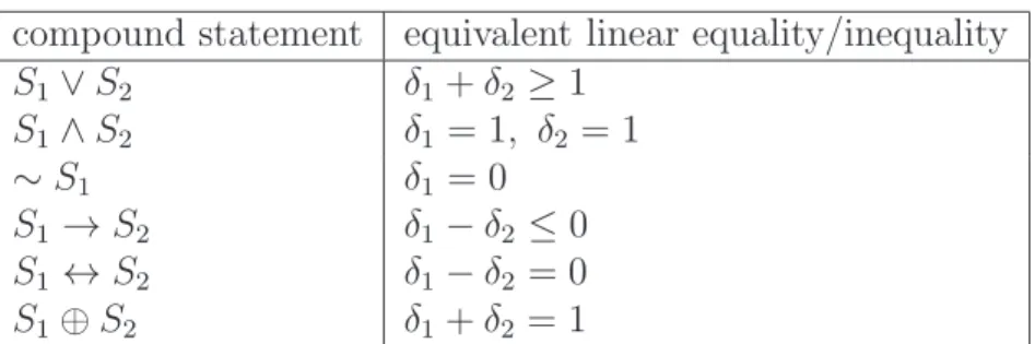
A propositional logic problem, where a statement S1 must be proved to be true given a set of compound statements containing literals S1, . . . , Sn, can be solved by means of a linear integer program. For this, logical variables denoted byδi (δi ∈ {0,1}) must be associated with the literalsSi. Then the original compound statements can be translated to linear inequalities involving the logical variables δi. A list of equivalent compound statements and linear equalities or inequalities taken from [153] is shown in Table 2.2.

S1 S2 ∼S1 S1 ∨S2 S1∧S2 S1 →S2 S1 ↔S2 S1⊕S2

T T F T T T T F

T F F T F F F T

F T T T F T F T

F F T F F T T F

Table 2.1: Truth table

compound statement equivalent linear equality/inequality S1∨S2 δ1+δ2 ≥1

S1∧S2 δ1 = 1, δ2 = 1

∼S1 δ1 = 0

S1 →S2 δ1−δ2 ≤0 S1 ↔S2 δ1−δ2 = 0 S1⊕S2 δ1+δ2 = 1

Table 2.2: Equivalent compound statements and linear equalities/inequalities

2.2 Positive (nonnegative) systems

The concepts and basic results in this short section are mostly taken from [22]. A function f = [f1 . . . fn]^T : [0,∞)ⁿ → Rⁿ is called essentially nonnegative if, for all i = 1, . . . , n, fi(x) ≥ 0 for all x ∈ [0,∞)ⁿ, whenever xi = 0. In the linear case, when f(x) = Ax, the necessary and sufficient condition for essential nonnegativity is that the off-diagonal entries of A are nonnegative (such a matrix is often called a Metzler-matrix).

(22)

Consider an autonomous nonlinear system

˙

x=f(x), x(0) =x₀ (2.10)

wheref :X →Rⁿis locally Lipschitz, X is an open subset ofRⁿandx0 ∈ X. Suppose that the nonnegative orthant [0,∞)ⁿ = Rⁿ+ ⊂ X. Then the nonnegative orthant is invariant for the dynamics (2.10) if and only iff is essentially nonnegative.

Quasi-polynomial and Lotka-Volterra models (section 2.3), and deterministic biochemical reaction networks (section 2.5) are well-known examples of essentially nonnegative systems.

2.3 Quasi-polynomial (QP) systems

2.3.1 Model form

Quasi-polynomial systems are systems of ODEs of the following form

˙

y_i =y_i l_i+ Xm

j=1

A_ij Yn

k=1

y^B_k^jk

!

, i= 1, . . . , n, (2.11) where y ∈ int(Rⁿ+), A ∈ R^n×m, B ∈ R^m×n, li ∈ R, i = 1, . . . , n. Furthermore, L= [l₁ . . . l_n]^T. Without the loss of generality we can assume that Rank(B) =n and m≥n (see [79]).

Let us denote the monomials of (2.11) as z_j =

Yn

k=1

y_k^B^jk, j = 1, . . . , m. (2.12) It can be easily calculated that the time derivatives of the monomials form a Lotka- Volterra system i.e.

˙

z_i =z_i(λ_i+ Xm

j=1

M_ijz_j), i= 1, . . . , m, (2.13) where M =B·A ∈R^m×m,λ= (B·L)∈R^m×1, and zi >0, i=1,. . . , m.

2.3.2 Transforming non-QP models into QP form

A wide class of nonlinear autonomous systems with smooth nonlinearities can be embedded into QP-form if they satisfy two requirements [76].

1. The set of nonlinear ODEs should be in the form:

˙

ys = X

is1,...,isn,js

ais1...isnjsy₁ⁱ^s1. . . y_nⁱ^snf(y)^j^s, (2.14)

y_s(t₀) =y_s⁰, s= 1, . . . , n

where f(y) is some scalar valued function, which is not reducible to quasi- monomial form containing terms in the form of Qn

k=1y^Γ_k^jk, j = 1, . . . , m with Γ being a real matrix.

(23)

2. Furthermore, we require that the partial derivatives of the model (2.14) fulfill:

∂f

∂ys

= X

es1,..,esn,es

b_e_s1_..e_sn_e_sy₁ê^s1. . . y_nê^snf(y)ê^s.

The embedding is performed by introducing a new auxiliary variable η =f^q

Yn

s=1

y_s^p^s, q6= 0. (2.15) Then, instead of the non-quasi-polynomial nonlinearityf we can write the original set of equations (2.14) into QP-form:

˙ ys=

ys

X

is1,...,isn,js

ais1...isnjsη^j^s^/q Yn

k=1

yⁱ_k^sk^−δ^sk^−j^s^p^k^/q

, s= 1, . . . , n, (2.16) where δsk = 1 if s = k and 0 otherwise. In addition, a new quasi-polynomial ODE appears for the new variable η:

˙ η=η

n

X

s=1

psy_s⁻¹y˙s+ X

isα,js

esα,es

aisα,jsbesα,esqη^(e^s^+j^s^−1)/q· Yn

k=1

yⁱ_k^sk^+e^sk^+(1−e^s^−j^s^)p^k^/q ,

α= 1, . . . , n. (2.17)

It is important to observe that the above embedding is not unique, because we can choose the parameterspsand q in (2.15) in many different ways: the simplest solution is to choose (ps = 0, s = 1, ..., n; q = 1). Since the embedded QP system includes the original differential variables yi, i = 1, . . . , n, it is clear that the stability of the embedded system (2.16)-(2.17) implies the stability of the original system (2.14).

2.3.3 Diagonal stabilizability and global stability of QP mod- els

By the global stability of QP systems, we mean stability with respect to the positive orthant. Let us assume that the model (2.13) has at least one equilibrium pointy^∗ in the strictly positive orthant, and let us denote the corresponding equilibrium in the monomial space by

z^∗ = [z₁^∗ z^∗₂ . . . z_m^∗]^T.

The following Lyapunov function candidate is often used when studying the global stability properties of (2.13) and (2.11) [146].

V(z) = Xm

i=1

ci

zi−z^∗_i −z^∗_i ln z_i z_i^∗

, (2.18)

where ci >0, i= 1, . . . , m.

It can be calculated that the time derivative of V satisfies V˙(z) = 1

2(z−z^∗)^T(M^TC+CM)(z−z^∗), (2.19)

(24)

where C = diag(c1, . . . , cm). This means that if the linear matrix inequality

M^TC+CM ≤0 (2.20)

can be solved for a positive definite diagonal matrix C, then any solution of (2.11) starting in the positive orthant is bounded and componentwise bounded away from zero [54], sinceV satisfies the requirements for being a Lyapunov function in the state-space of the original QP system (2.11), too. Naturally, in such a case z^∗ is a globally stable equilibrium point of (2.13) with Lyapunov function (2.18), and this implies the global stability of y^∗. In this case, we call M a diagonally stabilizable matrix. Furthermore, if the inequality (2.20) is strict, then the stability of z^∗ and y^∗ is asymptotic (M is diagonally asymptotically stabilizable). Moreover, it is shown it [54] that we can apply even milder conditions: if we assume (by appropriate ordering of the monomials) that the first n rows of B are linearly independent, then ci >0 for i= 1, . . . , nand cj ≥0 for j =n+ 1, . . . , mstill guarantees the global stability of y^∗.

Necessary and sufficient algebraic conditions of diagonal stabilizability are only available for 2×2 and 3×3 matrices [93], but it is true that a quadratic matrix M is diagonally stabilizable if and only if the LMI (2.20) has a positive definite diagonal solution, i.e the LMI

−(M^TC+CM)≥0, C >0 (2.21)

is feasible [14].

We remark that the diagonal stabilizability of a quadratic matrix is an important problem in different fields such as linear systems theory and also in other areas [95, 64, 93].

2.4 Generalized dissipative-Hamiltonian systems

The form of generalized dissipative Hamiltonian systems we will use is defined in [149].

In the autonomous case, this system class is given by the differential equations

˙

x= (J(x)−R(x))H^T_x(x), (2.22)

where x ∈ Rⁿ, H : Rⁿ 7→ R is the Hamiltonian function, J(x) is an n ×n skew symmetric matrix (i.e. J^T(x) = −J(x)), the energy conserving part of the system, and R(x) = R^T(x) is the so called dissipation matrix. H_x denotes the gradient of H (row vector).

The time derivative of the Hamiltonian function is H˙ =H_x(x)(J(x)−R(x))H^T_x(x) = Hx(x)J(x)H^T_x(x)

| {z }

0

−Hx(x)R(x)H^T_x(x). (2.23) In many cases, the J matrix satisfies the Jacobi equations

Xn

l=1

J_lj(x)∂J_ik

∂xl

(x) +J_li(x)∂J_kj

∂xl

(x) +J_lk(x)∂J_ji

∂xl

(x)

= 0, (2.24) i, j, k = 1, . . . , n

In this case, by Darboux’s theorem, around any point x0 where the rank of J(x) is constant it’s possible to find local coordinates

¯ x=

q1 . . . qk p1 . . . pk s1 . . . sl

T

(2.25)

(25)

such that J in the new coordinates has the form J(¯x) =





0 I^k 0

−I^k 0 0

0 0 0



 (2.26)

where I^k is a unit matrix of dimension k ×k, rank(J) = 2k, and n = 2k +l (see, e.g. [151]). J(¯x) in (2.26) is clearly symplectic if rank(J(x)) = n, n is even, and the integrability conditions in (2.24) are satisfied. We note that even if the conditions of the local coordinates transformation (2.25) are not fulfilled, the skew symmetricity ofJ still implies thaty^TJ(x)y= 0, ∀x, y ∈Rⁿ, which means thatHis a conserved quantity (first integral) of the system if R = 0. These facts motivate us to use the notion of generalized Hamiltonian systems and clearly show that this broader system class properly includes the class of classical Hamiltonian systems with symplectic structure.

It is visible from (2.23) that if y^TR(x)y≥0,∀x, y ∈Rⁿ(i.e. R is positive semidefi- nite), then the Hamiltonian function is nonincreasing. In this case, the model (2.22) is called a (globally) dissipative-Hamiltonian system. Of course, this property might be satisfied not globally, but only in some neighborhood of the equilibrium point (locally dissipative-Hamiltonian description). If there are no constraints about the local or global definiteness of R, the model is called a pseudo-Hamiltonian system [23]. It is important to note that in physical system models, the matrices J(x) and R(x) often reflect the physical structure or topology of the system [149].

2.5 Chemical reaction networks

2.5.1 Basic description of mass action reaction networks

The original physical picture underlying the reaction kinetic system class is a closed thermodynamic system with constant physico-chemical properties under isothermal and isobaric conditions, where chemical species Xi, i= 1, ..., ntake part inr chemical reactions. The system is assumed to be perfectly stirred, i.e. concentrated parameter in the simplest case. The specie concentrations xi = [Xi], i = 1, ..., n form the state vector, the elements of which are non-negative by nature.

The origin of mass action law lies in the molecular collision picture of chemical reactions. Here the reaction occurs when either two reactant molecules collide, or a reactant molecule collides with an inactive (e.g. solvent) molecule. Clearly, the probability of having a reaction is proportional to the probability of collisions, that is proportional to the concentration of the reactant(s).

A straightforward generalization of the above molecular collision picture is when we allow to have multi-molecule collisions to obtain elementary reaction steps in the following form [83, 155]:

Xn

i=1

αijXi → Xn

i=1

βijXi, j = 1, ..., r, (2.27) where the nonnegative integers αij, βij are the so-called stoichiometric coefficients of componentXi in thejth reaction. The linear combinations of the species in eq. (2.27), namely Pn

i=1α_ijX_i and Pn

i=1β_ijX_i for j = 1, . . . , r are called the complexes and are denoted by C1, C2, . . . , Cm. According to the extended molecular picture, thereaction

(26)

rate of the above reactions can be described as ρj =kj

Yn

i=1

[Xi]^α^ij =kj

Yn

i=1

x^α_i^ij , j = 1, ..., r, (2.28) where kj > 0 is the reaction rate constant (or reaction rate coefficient) of the jth reaction.

To further formalize the above description, following [49] and several other related works, we will also characterize CRNs with the following three sets.

1. S ={X₁, . . . , X_n} is the set of species or chemical substances.

2. C ={C₁, . . . , C_m} is the set of complexes. As it has been mentioned before, the complexes are represented as linear combinations of the species with nonnegative integer coefficients (see, eq. (2.27)).

3. R ={(C_i, Cj) | Ci, Cj ∈ C, and Ci is transformed to Cj in the CRN} is the set of reactions. The relation (C_i, C_j) ∈ R will be denoted as C_i → C_j. In this case, Ci is called the reactant or source complex, andCj is the product complex.

The nonnegative reaction rate coefficient is assigned to each reaction. When it is more convenient, we will index the reaction rate coefficients with a double index, i.e. kij denotes the rate coefficient of the reaction Ci→Cj.

During the numerical computations, the reaction rate coefficients of all possible reactions are often stored in matrices. In such a case, kij = 0 means that the reaction C_i → C_j is actually not taking place in the reaction network (i.e. (C_i, C_j)∈ R), and/ the corresponding directed edge (with zero weight) is naturally not drawn in the reaction graph. If the reactions Ci →Cj and Cj → Ci are present at the same time in a reaction network for some i, j then this pair of reactions is called a reversible reaction (but it will be treated as two separate elementary reactions in most of the forthcoming computations).

2.5.2 Graph representation of mass-action systems

The above description naturally gives rise to the following weighted directed graph structure [49] assigned to the CRN (2.27). The weighted directed graph D= (Vd, Ed) of a reaction network (simply called the reaction graph) consists of a finite nonempty set Vdof vertices and a finite set Edof ordered pairs of distinct vertices called directed edges. The vertices correspond to the complexes, i.e. Vd ={C₁, C2, . . . Cm}, while the directed edges represent the reactions, i.e. (C_i, C_j)∈E_d if complex C_i is transformed to Cj in the reaction network. The reaction rates kj for j = 1, . . . , r in (2.28) are assigned as positive weights to the corresponding directed edges in the graph. A walk in the reaction graph is an alternating sequence W = C₁E₁C₂E₂. . . C_k−1E_k−1C_kE_k where Ci ∈ Vd, Ei ∈ Ed for i = 1, . . . , k. W is a directed path if all the vertices in it are distinct. P is called a directed cycle if the vertices C1, C2, . . . , Ck−1 are distinct, k ≥3 andC1 =Ck.

A set of complexes {C1, C2, . . . , Ck} is a linkage class of a reaction network if the complexes of the set are linked to each other in the reaction graph but not to any other complex [50] (i.e. the individual linkage classes form the connected components of the directed graphD). Two different complexes are said to bestrongly linked if there exists a directed path from one complex to the other, and a directed path from the second

(27)

complex back to the first. Moreover, each complex is defined to be strongly linked to itself. A strong linkage class is a set of complexes with the following properties: each pair of complexes in the set is strongly linked, and no complex in the set is strongly linked to a complex that is not in the set. Aterminal strong linkage class is a strong linkage class that contains no complex that reacts to a complex in a different strong linkage class (i.e. there is no ”exit” from a terminal strong linkage class through a directed edge).

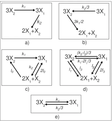
A reaction network is called reversible, if whenever the reaction C_i → C_j exists, then the reverse reaction Cj →Ci is also present in the network. A reaction network is called weakly reversible, if each complex in the reaction graph lies on at least one directed cycle (i.e. if complexC_j is reachable from complexC_ion a directed path in the reaction graph, thenCi is reachable fromCj on a directed path). If the corresponding forward and backward reaction pairs form a cycle in the directed graph of a reversible CRN, then this cycle of reversible edge-pairs will be called a circuit to distinguish it from a directed cycle. E.g. the CRN in Fig. 2.3 d) contains a circuit of length 3, while the CRNs in Figs. 2.3 a), b) and c) do not contain any circuit. By the structure of a CRN we simply mean the unweighted directed graph of a reaction network.

2.5.3 Differential equations of mass-action systems

There are several possibilities to represent the dynamic equations of mass action systems (see, e.g. [49, 69, 28]. The most advantageous form for our purposes is the one that is used e.g. in Lecture 4 of [49], i.e.

˙

x=Y ·Ak·ψ(x), (2.29)

where x∈Rⁿ is the concentration vector of the species, Y ∈R^n×m called the complex composition matrix stores the stoichiometric coefficients of the complexes,A_k ∈R^m×m contains the information corresponding to the weighted directed graph of the reaction network, and ψ :Rⁿ7→R^m is a monomial-type vector mapping defined by

ψj(x) = Yn

i=1

x^Y_i^ij, j = 1, . . . , m. (2.30) The exact structure of Y and A_k is the following. The ith column of Y contains the composition of complexCi, i.e. Yji is the stoichiometric coefficient ofCi corresponding to the specie Xj. Ak is a column conservation matrix (i.e. the sum of the elements in each column is zero) defined as

[Ak]ij =

−Pm

l=1,l6=ikil, if i=j

kji, if i6=j. (2.31)

Using the notions of the reaction graph, the diagonal elements [Ak]ii contain the negative sum of the weights of the edges starting from the nodeCi, while the off-diagonal elements [Ak]ij, i 6= j contain the weights of the directed edges (Cj, Ci) coming into Ci. Based on the above properties, it is appropriate to call Ak the Kirchhoff matrix orkinetics matrix of a reaction network.

To handle the exchange of materials between the environment and the reaction network, the so-called ”zero-complex” can be introduced and used which is a special complex with all the stoichiometric coefficients zero i.e., it is represented by a zero vector in the Y matrix (for the details, see, e.g. [49] or [26]).