Statistical process control in the evaluation of geostatistical simulations

(1)

Statistical process control in the evaluation of geostatistical simulations

János Geiger*

Department of Geology and Paleontology, University of Szeged, Szeged, Hungary Received: July 30, 2017; accepted: December 20, 2017

This paper deals with a question: how many stochastic realizations of sequential Gaussian and indicator simulations should be generated to obtain a fairly stable description of the studied spatial process? The grids of E-type estimations and conditional variances were calculated from pooled sets of 100 realizations (the cardinality of the subsets increases by one in the consecutive steps). At each pooling step, a grid average was derived from the corresponding E-type grid, and the variance (calculated for all the simulated values of the pooling set) was decomposed into within-group variance (WGV) and between-group variance (BGV). The former was used as a measurement of numerical uncertainty at grid points, while the between-group variance was regarded as a tool to characterize the geologic heterogeneity between grid nodes. By plotting these three values (grid average, WGV, and BGV) against the number of pooling steps, three equidistant series could be defined. The ergodic fluctuations of the stochastic realizations may result in some“outliers”in these series. From a particular lag, beyond which no“outlier”occurs, the series can be regarded as being fully controlled by a background statistical process. The number of pooled realizations belonging to this step/lag can be regarded as the sufficient number of realizations to generate. In this paper, autoregressive integrated moving average processes were used to describe the statistical process control. The paper also studies how the sufficient number of realizations depends on grid resolutions. The method is illustrated on a computed tomography slice of a sandstone core sample.

Keywords: geostatistics, statistical process control, ARIMA chart, sequential Gaussian simulation, sequential indicator simulation

*Corresponding address: Department of Geology and Paleontology, University of Szeged, Egyetem u. 2-6, Szeged H-6722, Hungary

E-mail:matska@geo.u‑szeged.hu

This is an open-access article distributed under the terms of theCreative Commons Attribution-NonCommercial 4.0 International License, which permits unrestricted use, distribution, and reproduction in any medium for noncommercial purposes, provided the original author and source are credited, a link to the CC License is provided, and changes–if any–are indicated.

DOI: 10.1556/24.61.2018.04 First published online February 28, 2018

(2)

Introduction

The basic paradigm of geostatistics is the belief that any geologic parameter (e.g., the porosity of a subsurface rock body) can be described by a multidimensional probability function, which is a collection of random variables, one per site of interest in the sampling space. A realization (e.g., a contour map of porosity) of this random function is deﬁned as a set of values that arises after obtaining one outcome for every distribution (Olea 1999).

In geostatistics, simulation commonly refers to the process of generating multiple realizations of a random function to obtain an acceptable numerical solution to a spatial problem. In such studies, hundreds of alternate models (called stochastic realizations) are generated and processed to produce a distribution of possible values for some critical parameter. In most of the geostatistical studies, these realizations are grids, which not only honor all of the input information but are also equally probable in the sense that any one of them is as likely a representation of the“true reality”as the others (Goovaerts 1999). In geostatistical applications, these realizations are used to describe the speciﬁc targeted multivariate distribution (e.g., the porosity of a subsurface rock body). The simplest form of the descriptive process relies on the calculations of, for example, the average spatial tendency and variance. They can be approximated by computing the arithmetic means and variance at each grid node (Journel and Deutsch 1993). Theﬁnal results are grids expressing the average spatial pattern (“E-type map”) and the stability of this pattern (“map of conditional variance”).

Obviously, uncertainty is always associated with the result. One can generally expect that the larger the number of stochastic realizations, the more precise the estimation of reality. In the other words, a modeler expects that an average porosity map (E-type estimation) will be “closer to the reality,”which is calculated from a greater number of stochastic realizations. Even the stability of this“closer-to-reality” grid is expected to be greater.

Thus, the problem of the number of sufﬁcient realizations to obtain a fair approxi- mation of the reality is quite an important question for modelers. Too few realizations will produce an average grid which is quite far from reality, whereas too many images will signiﬁcantly increase the CPU time of the already tedious geostatistical analysis.

Nevertheless, the issue of the number of realizations required to explore the space of uncertainty has received little attention. Goovaerts (1999) proposed the idea of creating subsets of increasing size through the random sampling of an initial set of 100 response values. This resampling created 100 subsets for each of the 99 possible sizes. For each subset, descriptive statistics were used to study the impact of the number of realizations.

He found that the extent of the space increases with the number of realizations, but at different rates depending on the response variable and simulation algorithm. Geiger et al.

(2010) generated 98 subsets of increasing size from 100 realizations. The first set contained thefirst three, the second did thefirst four realizations, and the 98th contained all 100 realizations. For each set, they calculated grid averages of the E-type estimations along with the between-group variance (BGV) and within-group variance (WGV).

(3)

They studied the limits of the sequences of these statistical properties within the framework of the stochastic convergence. The necessary number of realizations was defined by using Heine’s definition of convergence. Pyrcz and Deutsch (2014) concluded that the required number of realizations depends on (a) the aspect of uncertainty or the “statistic” being quantified and (b) the precision required for the uncertainty assessment. They used two parameters in their analysis: (a) the deviation, ΔF, in units of cumulative probability, from the reported quantile and (b) a parametertF, which was the fraction of times the true value will fall within±of the reported statistic.

In this context, they could derive the required number of realizations,L, to meet a certain speciﬁed standard, i.e., a speciﬁed ΔFand tF. Alternatively, the parametersF andtF

could be established for a givenL. That is, it was possible to calculate the uncertainty of their results due to a small number of realizations. Jakab (2017) realized that the desired structure of fair random sampling of the space of uncertainty is strongly analogous to the complete spatial randomness of spatial point processes, where the points are neither dispersed nor aggregated in space. Based on this analogy, she applied the normalized version of Ripley’s K-function and the L-function for the spatial inhomogeneous Poisson point process toﬁnd the optimal number of realizations.

All four of the approaches have several drawbacks and problems arising from the fact that only a limited number of realizations is available, and that ergodicﬂuctuation renders any generalization of the results difﬁcult.

Recently, Sancho et al. (2016) demonstrated a new approach in geostatistical analysis. This is the family of statistical process controls (SPC), by which one can differentiate“assignable”(“special”) sources of variation from“common”sources in a time series. Following the view of these authors, this paper focuses on the application of autoregressive integrated moving averages (ARIMA)-based SPC in the deﬁnition of the critical number of stochastic realizations.

The input data

The method is illustrated on a computed tomography (CT) slice of a sandstone core sample. The image and the corresponding data set (Fig. 1) consisted of 16,000 measured Hounsﬁeld Unit (HU) values arranged on a regular 125×128 grid. It was considered to be an exhaustive data set, which was sampled by a random set of 100 data locations. The corresponding values were treated as hard conditioning data.

The equality of the random and the exhausting set was conﬁrmed by a Q–Q plot.

Applied methods

Geostatistical sequential simulations (sequential Gaussian and indicator simulations) In theﬁrst step of the workﬂow, a sequential Gaussian simulation (SGS) and sequential indicator simulation (SIS) with 100 realizations were generated for the

(4)

random data set (Fig.2). Gaussian simulations are quite weak for honoring any lace- like geometry, whereas they are good in honoring small-scale heterogeneity (Srivastava 1990). In contrast, indicator simulations are strong in honoring and revealing lace-like geometry, but they are quite weak in describing small-scale heterogeneity (Olea 1999). Also, indicator simulations force the connectivity of all, originally discrete, geometric structures. The use of these two simulation approaches enabled us to study the effect of the simulation methods on the results.

Whatever property of a multidimensional random function is to be approached, the result strongly depends on the grid resolution applied in the simulation (e.g.,Journel and Deutsch 1993;Wilde and Deutsch 2010). Atfirst glance, it can be expected that the higher the resolution the smaller the scale of the heterogeneities that are revealed. However, it can also be admitted that any sequential simulation tends to introduce artifacts into the pattern of small-scale heterogeneities. In the sequential approaches, any node value can be counted for some hard data and for some previously simulated node values within the range of influence (Goovaerts 1999; Jakab 2016). Therefore, under the fixed range of influence, a small grid distance (high resolution) means that fewer hard and more simulated data are available for the estimation. This can result in a higher chance of locally deviating from the input statistics (Isaaks 1990;Pyrcz and Deutsch 2014;Jakab 2017). Using several different grid resolutions, the changing magnitude of these local deviations and their effect on the realizations could be examined. That is why the applied simulation methods were calculated onfive grid resolutions obtained by the methods suggested by Hengl (2006). The resolutions were the following: (a) 0.5×0.5, (b) 1×1, (c) 1.5×1.5, (d) 2.0×2.0, and (e) 2.5×2.5.

Fig. 1

The exhaustive and sampling data sets. (A) Original CT slice where the black dots indicate the locations of random sampling. (B) Comparison of the probability distributions of the exhaustive and sampling data sets

(5)

Deﬁnitions of pooled sets of realizations and their characterizations

The next step was the generation of pooled sets of realizations for thefive grid resolutions (Fig. 3). For both types of simulations with 100 realizations each, 98 subsets with increasing cardinality were created. Thefirst set contained thefirst three, the second comprised the first four, while the 98th contained all 100 realizations. In other words, the first subset of three realizations had three simulated values at each grid node, while the 98th contained 98 simulated values at each grid node. Generalizing this framework: ifN denotes the number of grid nodes (N=16,000) andj, j=1, 2,: : :, 98, represents the row number of the sets of pooled realizations defined above, then in thejsubset, there arejsimulated values which are nested within N grid nodes. This arrangement of the node values resembles the framework of one-way analysis of variance (ANOVA) (Miller and Khan 1962). In geostatistical analyses, this approach was applied by Webster et al.

(2002) for estimating the spatial scales of regionalized variables.

Fig. 2 Workﬂow

(6)

Deﬁnitions of averages in the one-way-ANOVA framework

For this framework, two types of averages can be derived. Theﬁrst is the average value for the all realizations. If the number of realizations isﬁxed tol, this average can be calculated fromlN grid nodes. In the remainder of this paper, we refer to this as grid average. The next type can be considered by the individual subsets of theNgrid nodes. Recall that after performinglsimulation at each of theNgrid nodes, there arel simulated values available. From these sets,Naverages can be derived, which will be referred to as node averages.

Variance decomposition

The total variance of the applied sequential simulation framework depends on two things. The ﬁrst is the variability around the grid average, while the second is the variances being characteristic around the node averages. In the terms of one-way- ANOVA, they are called BGV and WGV, respectively (Miller and Khan 1962).

The relation between these variance types is given by the so-called variance (σ²) decomposition. This states the following (Miller and Khan 1962): “if a sample contains N groups with the cardinality of n1, n2,: : :,nN, the members (subsets) of thel^thgroups arex^ðjÞ₁ ,x^ðjÞ₂ ,: : :,x^ðjÞ_l , then the total variance of these samples is the sum of WGV and BGV.”

σ²= 1 SUM

X^N

i=1

n_i·σ²i + 1 SUM

X^l

i=1

ðx_i−XÞ², (1)

where SUM= P_N

i=1n_i,X=_SUM¹ P_l

i=1

P_N

j=1x_ij,x_i=_n¹_iP_N

j=1x_ij.

Fig. 3

Elements of a statistical control chart

(7)

In Eq.(1), the ﬁrst member of the sum is called WGV. It measures the average deviation of individual values from the corresponding group average in the whole sample. The second member in Eq. (1) is the BGV. It is dedicated to measuring variance of the group averagesðx_i, i=1, 2,: : :,NÞaround the main averageðXÞ. The formalism of Eq.(1)can easily be adapted to our case. Let us suppose thatl realizations have been generated withNgrid nodes each. Letσ²^ðlÞbe the total variance of all the values generated in lsimulations. The number of groups is equal to the number of grid nodes,N. The number of samples in thej^thgroup (j≤N) corresponds to the number of realizations,l. SUM, which is the total number of simulated values in thelrealizations, takeslN.Xis the average calculated from thelNsimulated values, whilex_isði=1, 2,: : :,NÞare theNnode averages; each of them is calculated froml simulated values. This way, by applying some simpliﬁcations, Eq. (1)becomes

σ²^ðlÞ= 1 N

X^N

i=1

σ²i^ðlÞ+ 1 N

X^N

i=1

ðx^ðlÞ_j −X^ðlÞÞ², l=1, 2,: : :,N, (2)

In Eq. (2), the upper index ðlÞ shows that the expression goes for the ﬁrst l realizations.

From the above variance decomposition, WGV and BGV take the following forms for a given grid resolution:

WGV= 1 N

X^N

i=1

σ²i^ðlÞ, (3)

BGV= 1 N

X^N

i=1

ðx^ðlÞ_j −X^ðlÞÞ²: (4)

In this context, WGV measures the average variance of simulated values at grid nodes. BGV expresses the average variance of simulated values between grid nodes.

Some notes on convergence

Through the increasing number of pooled realizations, the“real”spatial distribution of the studied phenomena can be approached. One can expect that, for example, the map of average porosity calculated from, say, 100 realizations can better characterize the spatial distribution of porosity than that which was calculated from, say, 10 stochastic realizations. It can also be expected that these average porosity maps can differ signiﬁcantly from one another. However, the difference between two average porosity maps, which originated from 100 and 110 realizations, is not as perceptible as in the former case.

Recalling the fact that each porosity realization is a multivariate probability distribution, these characters of pooled realizations can be summarized in terms of convergence of probability distribution. In this context, convergence means that the

(8)

spatial data distribution tends“to be stabilized”when the cardinality of the pooled sets increases. It may also be true that this“stabilizing”process shows ergodicﬂuctuations.

There are two problems setting limits to the analytical study of this convergence. First, the analytical form of the multivariate probability distributions represented by the realizations is not known, except in the case of multi-Gaussian distributions. The second important problem is that the form and speed of convergence strongly depends on the grid resolution (Geiger et al. 2010).

This process can be studied by several methods (e.g.,Goovaerts 1999or Geiger et al. 2010). From among them, this paper uses the ARIMA-type SPC.

Statistical process control (SPC)

The next complex step in the workﬂow is SPC (Fig.2). This is a family of methods to monitor and control (quality control) a process using statistical methods (Shewhart 1931;Montgomery 1997;Oakland 2003).

SPC can be applied to any process where the “conforming product” (product- meeting speciﬁcations) output can be measured. The objective is to analyze data and detect anomalous values of the variable(s) analyzed.

In general, according to a certain tolerance margin and an objective value, two control limits are defined: an upper control limit (UCL) and a lower control limit (LCL). Their practical definitions depend on the type of SPC applied. In this study, UCL and LCL have been defined according to Eq.(6). If the measurements are within the UCL and LCL, there is not a non-random pattern in the distribution, and the process is under statistical control (Fig. 3). However, if there are points (measurements) outside the limits, then external causes influence the process, i.e., for these points, the process is not controlled (Montgomery 1997;Russo et al. 2012).

In this paper, the“objective value”is derived from the time-series model charac- terizing the shape of the average, WGV, and BGV series. The tolerance margins deﬁning the UCL and LCL are derived from the variability of actual data around the model curve, and the term“convergence”is replaced by the term“statistical control.” In this way, the minimum number of realizations by which one can generate a“stable” average or variance map is that cardinality of the pooled sets from which all the pooled sets end up being controlled (Figs3and4D).

In the practice of SPC analysis, there are three phases. The veryﬁrst phase is to understand the process and the speciﬁcation limits. In the second phase, the elimina- tion of assignable (special) sources of variation occurs, while the third phase is designed to monitor the ongoing process (Polhemus 2005). It should be noted that in this paper, the latter phase was not used.

ARIMA model and ARIMA chart

In this work, the ARIMA chart was used in SPC. The ARIMA model is a generalization of an autoregressive moving average (ARMA) model. ARIMA models

(9)

are applied in some cases where data show evidence of non-stationarity, where an initial differencing step (corresponding to the“integrated”part of the model) can be applied to reduce the non-stationarity (Box et al. 1994; Polhemus 2005;Russo et al. 2012).

In the abbreviation of ARIMA, the AR part indicates that the variable of interest is regressed on its own lagged (i.e., prior) values. The MA part indicates that the regression error is actually a linear combination of error terms whose values occurred contempo- raneously and at various times in the past. The I (for“integrated”) indicates that the data values have been replaced with the difference between their values and the previous values (and this differencing process may have been performed more than once).

In their most general form, ARIMA (p, d, q), these models consist of three characteristic terms: (a) a set of autoregressive terms (denoted by p), (b) a set of moving average terms or non-seasonal differences (denoted by d), and (3) a set of lagged forecast errors in the prediction equation (denoted by q). The general form of the model is as follows (Polhemus 2005):

Y_t=μ+Φ1·Y_t−1+ · · · +Φp·Y_t−p+e_t−Θ1·e_t−1−· · ·−Θq·e_t−q, (5) whereμis the constant,Φkis the autoregressive coefﬁcient at lagk,Θkis the moving average coefﬁcient at lagk, ande_t−kis the forecast error that was made at period (t−k).

The ARIMA charts procedure creates control charts for a single numeric variable where the data have been collected either individually (this version was used in this

Fig. 4

An example of the applied ARIMA charts. (A) Parameters of the selected model. (B) Explicit form of the selected model. (C) Parameters of the ARIMA chart. (D) ARIMA chart with the indication of the necessary (minimum) number of realizations

(10)

study) or in subgroups. It is constructed to describe the serial correlation between observations close together in time. Out-of-control signals are based on the deviations of the process from this dynamic time series model (Fig.3). In this chart, the data are drawn around a centerline located at the expected value,μ, with control limits at

μ±k·σ²: (6)

In this study,k= 1. The mean and standard deviation depend on the ARIMA model speciﬁcation (Polhemus 2005).

Figure4shows a typical example of the applied analysis with ARIMA charts. In Fig.4A, the components of thefitted significantARIMA(3,0,0) model is shown. The explicit form of this model is a linear combination of a constant, three autoregressive terms, and an error term (Fig.4B). The calculated centerline (average) and the UCL and LCL lines are shown in Fig.4C. Finally, in Fig.4D, the ARIMA chart can be seen, where the black dots indicate those parts of the series where severe deviations can be detected from theARIMA(3,0,0) model (Fig.4C). When the process does not trigger any deviation from the“detection rules”of the control chart, it is said to be“stable.” From a particular step, beyond which there is not any “outlier,”the series can be regarded as fully controlled by a background statistical process [in this case by the ARIMA(3,0,0) process]. The number of pooled realizations belonging to this step can be regarded as a sufficient number of realizations for generating purposes (Fig.4C).

In the ARIMA modeling approaches, Box–Cox transformations ensured the requirement of normality (Box and Cox 1964), and in the model selections, Nau’s train of thought was followed (Nau 2017). Obviously, the signiﬁcance of the selected ARIMA model must be checked. For this purpose, partly statistical tests and partly the residual autocorrelations of the ARIMA model were used (Polhemus 2005).

Demonstrating the method on the example of a CT slice

The image and the corresponding data set consisted of 16,000 HU values measured on a 125×128 regular grid. From this data set, 100 data locations and the corresponding measurements were randomly chosen as the input data (Fig.1). With this, a random set of sequential Gaussian and SIS were generated.

In the case of SGS, after the normal score transform of the input data, the spatial continuity was modeled using three empirical directional variograms. The variogram modeling was performed according to the Matheronian method (Journel and Huijbregts 1978). Theﬁnal model was the nested one with the combination of an exponential (main direction: 82°; range: 29; contribution: 0.70; anisotropy: 0.36) and a Gaussian (main direction: 47°; range: 53; contribution: 0.13; zonal anisotropy) models with 0.17 nugget effect (Fig. 5). The goodness of the ﬁtted model was evaluated according to Pannatier (1996). The realizations were back transformed.

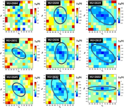
The SIS were based on nine cut-off values discretizing the original data distribution (Fig. 6). The corresponding variogram maps showed a quite large diversity of

(11)

Fig. 5

Variography for the sequential Gaussian simulations. (A) Variogram map of the data. (B) Variogram models in three directions. (C) Variogram map of the model

Fig. 6

Deﬁnitions of cut-offs for the sequential indicator simulations

(12)

continuity directions (Fig.7). The models of the indicator variograms were deﬁned as spherical ones with different ranges and anisotropies.

The simulation results were rendered onﬁve grid resolutions deﬁned according to Hengl (2006). They were 0.5×0.5, 1.0×1.0, 1.5×1.5, 2.0×2.0, and 2.5×2.5.

Figure 8 shows the CT-image and the E-type estimations calculated from 100 realizations of SGS and SIS methods for ﬁve grid geometries. The two simulation approaches emphasized two different characters of the original CT image. SGS models were forced to create rounded patches, whereas the indicator models highlighted the linear features. However, except for the lower right part, both solutions described the general outline quite well (Fig. 8). Figure 8 also provides evidence that theﬁner the grid resolution, the more details can be seen in the maps.

Altogether, 98 pooled sets were defined for each type of simulations and grid resolutions. Thefirst contained thefirst three, the second did thefirst four, etc., and the 98th consisted of 100 realizations. For these sets, three statistics were calculated for

Fig. 7

Variogram map of the deﬁned indicator variables

(13)

each grid resolution: (a) the grid average of the E-type estimation; (b) the WGV; and (c) the BGV.

Figure 9 shows the ARIMA charts of the grid averages of E-type estimations calculated from the pooled sets with increasing cardinality. With the exception of the ﬁnest grid resolutions, the grid averages approach their statistically controlled states in monotonously increasing ways. The accepted ARIMA models belonging to the indicator simulations contained only autoregressive components. The models of Gaussian simulations obtained for the 0.5×.0.5 and 1.5×1.5 resolutions contained moving average terms as well. The number of lags of the autoregressive components were smaller for the Gaussian simulations than for those of indicator simulations (Fig.9). The average of the ARIMA process changed wavily with the coarsening grid resolutions, though in the general tendency, the averages increased with the decreasing grid resolution (Fig. 10A).

The largest grid average belonged to the 2.0×2.0 resolution, whereas the smallest average characterized the 1.5×1.5 grid geometry. It was also characteristic that the indicator simulations generated smaller grid averages than the Gaussian simulations (Fig.10A). The widths of the control intervals (the difference between UCL and LCL)

Fig. 8

E-type estimations based on 100 realizations in the sequential Gaussian and in the sequential indicator simulations

(14)

Fig. 9

ARIMA charts of the grid averages of E-type estimations coming from SIS (left column) and SGS (right column)

(15)

are quite similar for both simulation methods (Fig.10B). In the sequential simulations, they showed a gently decreasing tendency toward the coarsening grid resolutions. In contrast, they are generally increased in the Gaussian simulations. Figure10Bshows that in the indicator approaches, the narrowest interval belonged to the coarsest grid resolution (2.5×2.5), whereas in the Gaussian approaches, the narrowest interval characterized theﬁnest grid geometry (0.5×0.5). In the cases of indicator simulations, the minimum number of realizations from which the ARIMA processes have become controlled showed an increasing decreasing tendency with the decreasing grid resolution. In contrast, this number decreased with the decreasing resolutions in Gaussian simulations (Fig.10C). It should be noted, in Fig.10C, that the numbers on thex-axes denote the row numbers of the sets of the pooled realizations. Since theﬁrst set contained three realizations, the actual number of realizations belonging to thei^th set is (i+3). For the indicator simulations, the smallest number of necessary realizations was 22, which belonged to the 1.5×1.5 resolution. In the case of Gaussian simulation, it was 16 relating to the coarsest grid. The largest number of realizations needed for being controlled was 67 in the case of indicator approaches, and was only 38 for Gaussian simulations (Fig.10C).

The ARIMA charts of WGV demonstrated that the computational heterogeneities moved toward their controls, with a monotonously increasing tendency with the increasing number of realizations (Fig. 11). In the indicator simulations, the

Fig. 10

Summarizations of the results derived from the ARIMA charts of the grid averages of the E-type estimations in the functions ofﬁve grid resolutions. (A) Centerline values in the functions of grid resolutions. (B) Widths of the control intervals in the functions of grid resolutions. (C) Required minimum number of realizations in the functions of grid resolutions

(16)

Fig. 11

ARIMA charts of the within-group variances coming from SIS (left column) and SGS (right column)

(17)

autoregressive components of the ARIMA models contained only one lag. That is, each value is controlled by only one former one. This is aﬁrst-order autoregressive model. Only the model for the 1.0×1.0 grid resolution contained a moving average term (Fig.11). In the case of Gaussian simulation, all the ARIMA models were (3,0,2)- type, independently of the grid resolutions (Fig. 11).

The centerlines of the ARIMA models obtained for the indicator simulations were smaller than those of Gaussian approaches. Also, the averages did not vary with the grid resolutions (Fig.12A). The widths of the control intervals were the narrowest for the 1.0×1.0 grid in the indicator simulations, while the narrowest interval belonged to the coarsest grid resolution in the Gaussian simulations (Fig. 12B). The necessary number of realizations for reaching a controlled state was 10 in Gaussian simulations and was 3 in the indicator methods (the corresponding row numbers of pooled sets are 8 and 1 as shown in Fig.12C). Thus, among the Gaussian simulations, the 1.5×1.5 and all the coarser grids required the smallest number of pooled realizations to stabilize the computational heterogeneity. However, in the indicator approaches, the computational heterogeneity became stable after three realizations in the coarsest grid resolution.

In the cases of BGV, in both the indicator and Gaussian approaches, the ARIMA model of the 1.0×1.0 resolution was the type ofARIMA(2,0,0), i.e., a second-order autoregressive model (Fig.13).

Fig. 12

Summarizations of the results derived from the ARIMA charts of the within-group variances (WGV) in the functions ofﬁve grid resolutions. (A) Centerline values in the functions of grid resolutions. (B) Widths of the control intervals in the functions of grid resolutions. (C) Required minimum number of realizations in the functions of grid resolutions

(18)

Fig. 13

ARIMA charts of the between-group variances coming from SIS (left column) and SGS (right column)

(19)

With the exception of this geometry, all the other models could be characterized by a linear combination of aﬁrst-order autoregressive and a second-order moving average models. The indicator simulations showed larger WGV than the Gaussian models. In both simulations, the WGV increased a bit with the increasing grid–node distances (Fig.14A). The variability of the width of the control interval was very low in the case of Gaussian simulations, and it showed a kind of “dumped” wavy trend with the coarsening grid resolutions in the indicator approaches (Fig. 14B). The necessary number of realizations decreased in the twoﬁnest resolutions; from the 1.0×1.0 grid to the coarsest resolution, these numbers increased (Fig.14C).

In the indicator and Gaussian simulations, the largest necessary number of simulation to reach a controlled model was 48 and 36, respectively. In both cases, the corresponding grid resolution was 2.0×2.0. In both groups of simulations, the 1.0×1.0 resolution was characterized by the smallest necessary number of realizations. They were 6 in the indicator and 11 in the Gaussian cases (Fig.14C).

The necessary number of realizations, by parameter types and simulation methods, are summarized in Table1. Obviously, a simulation result can be regarded as being fully controlled only if all the studied parameters are controlled. In the case of 0.5×0.5 resolution and SIS, the E-type estimation needed 42 realizations to be controlled by the corresponding ARIMA model. This number was 29 for the WGV and 35 for the BGV.

Thus, after generating at least 42 stochastic realizations, all three parameters are

Fig. 14

Summarizations of the results derived from the ARIMA charts of the between-group variances (BGV) in the functions ofﬁve grid resolutions. (A) Centerline values in the functions of grid resolutions. (B) Widths of the control intervals in the functions of grid resolutions. (C) Required minimum number of realizations in the functions of grid resolutions

(20)

controlled. When applying Gaussian simulation to the same grid resolution, the E-type grid, WGV, and BGV required 89, 10, and 20 realizations (Table1, row 0.5×0.5). That is, this type of simulation needed 89 realizations to be controlled. The numbers in the

“Final”column of Table1were derived in this way. It can be seen that the smallest number of realizations was needed by the SGS on 2.5×2.5 grid resolution and the largest number of realizations belonged to this simulation method on the 0.5×0.5 resolution.

If we put these numbers in ascending order by the grid resolutions and simulation methods (Table2), the result can be used to study how the simulation results have been affected by the grid resolutions. For example, in the case of 0.5×0.5 resolution, when SIS was applied,ﬁrst WGV stabilized, then came the BGV, andﬁnally the E-type grid (Table2, row of 0.5×0.5, columns“SIS”). In the Gaussian simulation, the order was the same. The column titled as“Final”in Table1has the same meaning as in Table2.

Table 1

Necessary number of realizations

Grid size

E-type Computation (WGV) Geology (BGV) Final

SIS SGS SIS SGS SIS SGS SIS SGS

0.5×0.5 42 89 29 10 35 20 42 89

1.0×1.0 45 54 24 19 4 8 45 54

1.5×1.5 20 39 43 8 21 12 43 39

2.0×2.0 36 32 29 8 34 46 36 46

2.5×2.5 65 22 1 8 22 20 65 22

SIS: sequential indicator simulation; SGS: sequential Gaussian simulation; WGV: within-group variance;

BGV: between-group variance

Table 2

Rank of properties being controlled

Grid size

E-type Computation (WGV) Geology (BGV) Final

SIS SGS SIS SGS SIS SGS SIS SGS

0.5×0.5 3 3 1 1 2 2 42 89

1.0×1.0 3 3 2 2 1 1 45 54

1.5×1.5 1 3 3 1 2 2 43 39

2.0×2.0 3 2 1 1 2 3 36 46

2.5×2.5 3 3 1 1 2 2 65 22

(21)

Discussion and conclusion

Geiger et al. (2010) interpreted WGV as a measure of“computational heterogeneity,”since it expresses the average variability of the simulated values at the grid nodes.

The BGV measures the variability of the grid–node averages. This spatial variability is sensitive, although not exclusively, to the spatial variability of the geologic process formed by the property studied. This is why they have interpreted BGV as“geologic heterogeneity.”

On the basis of these thoughts, an“ideal”order of the property stabilizations can be deﬁned in the following way. To begin with, the computational heterogeneity (WGV) should become stabilized (controlled by a statistical process). This may ensure that the forthcoming results will not be affected by computational artifacts. For example, in the case of Gaussian simulation, the decreasing ratio between the number of data values and the number of formerly simulated node values may cause unrealistic estimations.

Second, the geologic heterogeneity (BGV) should become controlled. This means that (a) all the signiﬁcant variabilities are considered, and that (b) the succeeding realizations will produce only denser information, without providing any new results. Consequently, the grid average of the E-type estimation should be last to become stabilized.

In the presented example, this“ideal order”characterizes the 0.5×0.5, 2.0×2.0 and 2.5×2.5 resolutions in the indicator simulations, and the 0.5×0.5, 1.5×1.5 and 2.5×2.5 grid systems in the Gaussian simulations (Table3). The smallest number of realizations belongs to the 2.5×2.5 grid in the group of indicator simulations and to

Table 3

Rank of orders in which simulations become controlled

Simulation and grid size Computation (WGV) Geology (BGV) Grid average SIS: 0.5×0.5

1 2 3

SGS: 0.5×0.5 SGS: 1.5×1.5 SIS: 2.0×2.0 SIS: 2.5×2.5 SGS: 2.5×2.5 SIS: 1.0×1.0

2 1 3

SGS: 1.0×1.0

SIS: 1.5×1.5 3 2 1

SGS: 2.0×2.0 1 3 2

(22)

the 0.5×0.5 grid in the group of Gaussian simulation. They are 42 and 22, respectively.

Any method has some advantages and some limitations. The application of SPC may provide the following advantages: (a) it can be applied to any distribution or uncertainty parameters derived from the simulation results (e.g., interquartile range, Shannon-entropy, etc.); (b) it takes into consideration the ergodicﬂuctuations; and (c) it does not rely on the hypothesis that the actual number of realization is sufﬁcient to understand the behavior of the series in the limit.

However, the suggested process also has some limitations: (a) the necessary number of realizations strongly depends upon the speciﬁcation of the ARIMA model (the process does not give a unique result); (b) the demonstrated process does not provide any information about how fair the sampling of the space of uncertainty is; and (c) this process only gives information about the grid averages and is not sensitive to any connectivity properties. With the above detailed advantages and limitations, the presented method can be useful in the uncertainty studies of any 2D geologic models, since it can provide that number of stochastic realizations from which, for instance, E-type estimation can reasonably be calculated without redundancy.

References

Box, G.E.P., D.R. Cox 1964: An analysis of transformations.–Journal of the Royal Statistical Society, Series B (Methodological), 26/2, pp. 211–252.

Box, G.E.P., G.M. Jenkins, G.C. Reinsel 1994: Time Series Analysis. Forecasting and Control.–Prentice-Hall International, Princeton, NJ, 619 p.

Geiger, J., T. Malvi´c, J. Horváth, K. Novak-Zelenika 2010: Statistical characters of realizations derived from sequential indicator simulation. – Proceedings of 14th Annual Conference of the International Association for Mathematical Geosciences, IAMG 2010, Budapest, 17 p.

Goovaerts, P. 1999: Impact of the simulation algorithm, magnitude of ergodicﬂuctuations and number of realizations on the spaces of uncertainty ofﬂow properties.–Stochastic Environmental Research and Risk Assessment, 13/3, pp. 161–182.

Hengl, T. 2006: Finding the right pixel size.–Computer & Geosciences, 32, pp. 1283–1298.

Isaaks, E.H. 1990: The application of Monte Carlo methods to the analysis of spatially correlated data.–PhD thesis, Stanford University, Stanford, 426 p.

Jakab, N. 2016: Uncertainty assessment based on scenarios derived from static connectivity metrics.–Open Geosciences, 8/1, pp. 799–807.

Jakab, N. 2017: Stochastic modeling in geology: Determining the sufﬁcient number of models.–Central European Geology, 60/2, pp. 1–17.

Journel, A.G., C.V. Deutsch 1993: GSLIB: Geostatistical Software Library and User’s Guide.–Oxford University Press, Oxford, 369 p.

Journel, A.G., Ch.J. Huijbregts 1978: Mining Geostatistics.–Academic Press, London, 600 p.

Miller, R.L., J.S. Khan 1962: Statistical Analysis in the Geological Sciences.–John Wiley and Sons, New York, pp. 164–144.

Montgomery, D.C. 1997: Introduction to Statistical Quality Control.–John Wiley and Sons, New York, 759 p.

(23)

Nau, R. 2017: ARIMA models for time series forecasting.–In: Nau R. (Ed): Statistical Forecasting: Notes on Regression and Time Series Analysis. Duke University, Durham. http://people.duke.edu/~rnau/

Notes_on_nonseasonal_ARIMA_models–Robert_Nau.pdf.

Oakland, J.S. 2003: Statistical Process Control.–Butterworth-Heineman, Oxford, 460 p.

Olea, R. 1999: Geostatistics for Engineers and Earth Scientists.–Springer, Boston, 303 p.

Pannatier, Y. 1996: Variowin: Software for Spatial Data Analysis.–Springer-Verlag, New York, 91 p.

Polhemus, N.W. 2005: How To: Construct a Control Chart for Autocorrelated Data.–StatPoint Technolo- gies, Herndon, 16 p.

Pyrcz, J.P., C.V. Deutsch 2014: Geostatistical Reservoir Modeling.–Oxford University Press, Oxford, 449 p.

Russo, S.L., M.E. Camargo, J.P. Fabris 2012: Applications of control charts ARIMA for autocorrelated data.–In: Nezhad M.S.F. (Ed): Practical Concepts of Quality Control. InTech, Rijeka, pp. 31–53.https://

www.intechopen.com/books/practical-concepts-of-quality-control/applications-of-control-charts-arima- for-autocorrelated-data.

Sancho, J., C. Iglesias, J. Pineiro, J. Martínez, J. Pastor, M. Araújo, J. Taboada 2016: Study of water quality˜ in a Spanish river based on statistical process control and functional data analysis.–Mathematical Geosciences, 48, pp. 163–186.

Shewhart, W.A. 1931: Economic Control of Quality of the Manufactured Product. – Van Nostrand, New York, 501 p.

Srivastava, R.M. 1990: An application of geostatistical methods for risk analysis in reservoir management.– SPE Paper, 20608, pp. 825–834.

Webster, R., S.J. Welham, J.M. Potts, M.A. Oliver 2002: Estimating the spatial scales of regionalized variables by nested sampling, hierarchical analysis of variance and residual maximum likelihood.– Computer & Geosciences, 32, pp. 1320–1333.

Wilde, B., C.V. Deutsch 2010: Data spacing and uncertainty: Quantiﬁcation and complications. – Proceedings of 14th Annual Conference of the International Association for Mathematical Geosciences, IAMG 2010, Budapest, 24 p.