SAVER TYPES: AN EVOLUTIONARY-ADAPTIVE APPROACH
1GERGELY VARGA1 – JÁNOS VINCZE2
1Department of Macroeconomics, Corvinus University of Budapest, Hungary Email: gergely.varga@uni-corvinus.hu
2Department of Mathematical Economics and Economic Analysis, Corvinus University of Budapest, Hungary and
Institute of Economics, Center for Economic and Regional Studies of the Hungarian Academy of Sciences, Budapest, Hungary
E-mail: janos.vincze@uni-corvinus.hu
We set up an agent-based macro-model that focuses on the consumption-saving decision. Agents do not maximize utility, but their behaviour features certain “rational” aspects of human choice based on the idea of ecological rationality. Three qualitatively different saving strategies are de- fi ned: 1, buffer stock saving (prudent and forward looking); 2, permanent income saving (forward looking without prudence); and 3, myopic saving (caring only about immediate consumption). It is found that prudent saving behaviour becomes prevalent when the selection pressure is very high, but an economy comprising only prudent households tends to accumulate capital in excess of what is implied by the Golden Rule. Lowering the intensity of evolutionary forces results in more diver- sity in saver types, and, somewhat puzzlingly, may be socially benefi cial in some sense.
Keywords: agent-based macro-model, bounded rationality, evolutionary learning, saving types JEL codes: C69, E21
1 We are grateful for valuable comments by András Simonovits and István Kónya. This study was funded by the grant OTKA K 108 658 of the Hungarian government.
1. INTRODUCTION
Saving is one of the central themes in economics. In growth theory it is through savings that nations become rich, although it was recognized that too much saving can harm consumption (the celebrated problem of dynamic inefficiency, see e.g.
Blanchard – Fischer, 1989). Short and medium term fluctuations in savings are important in business cycle analysis, and Akerlof and Shiller (2010: Chapter 10.) suggested that longer term waves in macroeconomic variables may be due to unstable saving behaviour in the long run. In addition, saving behaviour exhibits heterogeneity across time and nations. The existence of different saving rates across households is an important issue in the economics of poverty (Banerjee – Duflo 2011: Chapter 8), and is thought to have bearing on the ever changing wealth distribution within developed countries (Piketty 2014).
In this paper we contribute to the theory of long term interactions between sav- ings, income and consumption. Specifically, two issues are targeted. First, what are the forces that can lead to over- or under-accumulation, where these terms are understood relative to the Golden Rule principle? Second, can changes in saving behaviour generate “arbitrary” long term fluctuations in the productive capabili- ties of an economy, as Akerlof and Shiller suggested?
Section 2 looks at the literature on long term capital accumulation and saver types, and outlines our approach for answering the two questions raised above.
Section 3 presents the model, its parameterization and the simulation settings. Sec- tion 4 contains the basic findings via simulation exercises. Section 5 concludes .
2. LESSONS FROM THE LITERATURE
The possibility of dynamic inefficiency, i.e. accumulating capital in excess of the Golden Rule level (at which the net marginal product of capital equals the growth rate), emerged as a possible feature of overlapping generations models (Blanchard – Fischer 1989: 103–104). Whereas in models with infinitely living maximizing agents impatience drives savings below the level consistent with long-run con- sumption maximization, when agents have finite lives and must provide for them- selves in their old-age, they may find it rational to keep a stock of capital with a net return below the growth rate of the economy. If the necessity for self-provision (“supported” by low capital productivity) outweighs impatience, the equilibrium outcome may not be Pareto-efficient, despite market clearing and individual ra- tionality. Thus either under- or over-saving can be the outcome in traditional mod- els, due to the opposing forces of short-sightedness and “induced” prudence.
A closer inspection of national saving rates hints at puzzling facts about sav- ings in the long run. Akerlof and Shiller (2010) pointed out an attribute they call the “arbitrariness” of saving. Contemporaneously national savings rates as high as 1/3 coexist with negative ones. Capriciousness can be detected over time, too.
The personal savings rate in the US was reduced from 10% in the early 1980s to near zero rates in the 21st century. Akerlof and Shiller notice also the variability of savings rates across individuals resulting in huge differences in retirement wealth, and emphasize the inability of the traditional theory to account for this fact. Their preferred explanation is “Animal Spirits”, but they do not explain what it means exactly. They muster observations indicating that savings decisions are made on
“irrelevant cues”, and their anecdotal description of the role of stories (or culture) seems plausible. But how irrelevant cues can play a role in such an important decision, and how saving culture is shaped and changed are left unanswered.
Traditional economics reduces the explanation of savings behaviour to ex- ogenous variations in preferences and technology (including demographics).
Therefore, when apparently large changes are detected in saving rates, causes are looked for along these lines. For instance, Dobrescu et al. (2012) proposed models to elucidate the large declines in savings rates in developed countries, and concluded that the cause must be shifts in social preferences. This explanation, naturally, leaves open the question why preferences have been unstable.
The traditional utility maximizing theory of saving, originating in Fischer (1930), developed several models for rational households. Early theories disre- garded non-diversifiable income risk, therefore risk-taking did not play a signifi- cant role in them. A general result was that the marginal utility of consumption follows a random walk, and the response of consumption to permanent shocks is much stronger than to temporary ones. There were empirical studies that seemed to confirm that “certainty equivalent” households indeed exist (e.g. Hall – Mishkin 1982). Later researchers developed theories emphasizing non-diversifi- able labour income risk, and studied its interaction with prudent preferences. The buffer-stock theory of saving comes from this literature (see Carrol – Summers 1991). The main result here is that households’ behaviour can be characterized by a desired savings/income ratio. Buffer stock savers adjust consumption to get as close as possible to this target. This kind of behaviour leaves more room for the effects of non-permanent income, and appears to correspond partly to available evidence (see Carroll 1997).
Empirical modelling of saving had to face the problem of more individual het- erogeneity than that implied by utility maximizing agents. There is a long empiri- cal tradition that separates people into two groups: those whose behaviour can be described as “fully rational”, and those who seem to behave in a purely present-
oriented manner (see for instance Hall – Mishkin 1982). Whether the latter group behaves rationally but under constraints, or suffer from myopia, has always been an open question. Anyway, the distinction between these two fundamentally dif- ferent types of consumers was born on purely empirical grounds.
A modern variant of “irrational” consumption behaviour theory makes use of psychological findings about hyperbolic time discounting to give a theoretical ac- count of this “duality” in saving. This theory was rendered in its now usual format by Laibson (1997). Here the distinction is between rational long-run maximizers, and naive agents who have time-inconsistent preferences. Some more recent the- ories are based on other psychological theories according to which people have a dual-self, and are, sometimes, unable to recognize their best long-run interests (Fudenberg – Levine 2006). A related observation is made in Banerjee and Duflo (2011: Chapter 8) where the authors consider the baffling fact that though many poor people over the world might increase their well-being substantially with the help of a little bit more saving, there are only a few who accomplish this. Ban- erjee and Duflo enlist several explanations, and favour one that rests on the lack of self-control coupled with positive biological feedback. From their description we underline one important point: people say frequently that money cannot be kept at home, because there will always be some irresistible temptation to spend it. Our interpretation is that many people disburse money without much regard to the future.
All of these theories rely on a persistent coexistence of rational and irrational behaviour with respect to saving, while ignore the question why people cannot learn to act rationally, or why evolution cannot eradicate an apparently inferior behavioural pattern.
3. THE MODEL
As we focus on long-term issues, income and its primary distribution are de- termined on the supply side. The model has a simple production-distribution framework based on neoclassical assumptions regarding production, labour and physical capital services markets. Agents plan their consumption level in each pe- riod in accordance with their types (and subtypes), but, like in other agent-based macro-models, there is no in-built equilibrating mechanism, thus plans may turn out to be infeasible. Therefore, there must exist an (imperfect) credit market that intermediates between plans and actual consumption. The order of subsections follows the order of events in a given period: 3.1. production and the distribution of primary income, 3.2. planning of consumption, 3.3. the opening of the credit market and the determination of consumption, borrowing and physical capital
accumulation, 3.4. evolutionary learning. Then in subsection 3.5. the basic simu- lation setting is presented.
3.1. The production-distribution side
The production – primary income distribution side of the model follows the model in Aiyagari (1994), a version of Bewley-type models (see Chapter 17 in Ljungqvist – Sargent 2004), which have been studied to find out how incomplete markets influence equilibria in dynamic general equilibrium frameworks. Saving opportunities include private loans and physical capital. Our setting differs from traditional Bewley-type models in the way asset markets clear, and, most impor- tantly, in the behaviour of households.
There exist N ex ante identical, infinitely living dynasties of households. The labour supply of each dynasty (from now on dynasties are called either agents or households) is characterized by the same two-state Markov-chain, with the transition matrix in Table 1.
Table 1. Transformation matrix of households
L1 L2
L1 p 1 – p
L2 1 – q q
where L1< L2.
Individual labour supplies are independent, thus, if the number of agents is large, aggregate labour supply uncertainty is almost nil, though individual uncer- tainty can still be substantial.
The economy’s aggregate production function is of the Cobb-Douglas type, with aggregate labour and capital as its arguments, and α as capital’s share:
1
t t t
Y K Lα α
1 N
t tk
k
L L
1
,
N
t tk
k
K K
where Lt is aggregate labour, Ltk is labour supply of household k, Kt is aggregate physical capital, Ltk is capital owned by household k, and Yt is aggregate output.
Capital depreciates at rate δ per period.
The number of households and the parameters of the Markov-chain uniquely determine long-run average labour supply (L). We know that in the Cobb-Douglas case without uncertainty the Golden Rule savings rate is α, and the corresponding levels of capital and consumption can be expressed as
1
( )1
K α αL
δ
1
1 ,C α K Lα α
respectively. Below we will make use of these reference values when reporting results of simulation exercises.
Labour markets always clear, and work is rewarded according to its marginal product. Therefore the wage rate (wt) and the compensation of capital services (rtK) can be expressed explicitly as
1
tt
t
w Y
L
α
K t.
t t
r Y K
α
At the beginning of each period idiosyncratic labour supply shocks material- ize, then production and the distribution of primary income take place.
We need only to derive individual consumption and net credit (satisfying mar- ket clearing) in each period. From this data one can compute next period capital stock, both individually and in the aggregate. In the next subsection we describe how consumption is determined at any given array of individual consumption plans.
3.2. Consumption, capital accumulation and the credit market
Net wealth (Atk) and current income (Itk) for each agent are defined as:
tk tk tk tk
A K B D
K ,
tk t tk t tk t tk tk
I w L r δ K r B D
where rt is the rate of interest on private loans, Btk ≥ 0 is credit to other house- holds, and Dtk ≥ 0 is debt due to other households (see below about lending and borrowing). We will make use of the concept of cash-in hand (TW)
tk tk tk.
TW A I
After planning consumption each agent behaves identically, independently of its type. Essentially each household executes its consumption plan whenever own funds allow it. If not, the household tries to raise credit in order to fulfil the plan, though it may be restricted by a debt constraint.
In formulas, if
P
tk tk
C TW then
P,
tk tk
C C
and the household’s supply of funds (Wt + 1,k) becomes
1, ,
t k tk tk
W TW C while its borrowing demand is
1, 0.
t k
D Otherwise:
1, 0
t k
W
, 1 ,
P
tk tk tk Dt
C min C TW
where Dt + 1 is the debt constraint (see below).
In this case the borrowing demand of household k is:
1, 1, P 0.
t k t tk tk
D min D C TW
The credit limit is set as a percentage of current labour income in the “bad”
labour supply state (L1).
1, t 1,
t k w
D κ L
where κ is a parameter that determines the softness of the limit.
The interest rate is determined as
2
1 t K .
t t t
t
r D r
ω Y δ
where ωt ω is a uniformly distributed random variable. Thus rt + 1 is always at least as large as rtK – δ, and the “premium” increases when the debt ratio t
t
D Y of the economy is higher, reflecting that lending is riskier than owning physical capital, and implying that to get credit people must pay a premium to those who have positive wealth, and may lend.
If the feasibility condition
1, 1,
t j t j
j j
W D
is satisfied, the supply of funds is consistent with the demand for loans. In that case
1,
1, 1,
1, t j,
j
t k t k
t j
j
B W D
W
and
1, 1, 1, .
t k t k t k
K W B
Thus the portfolio weights with respect to credit and physical capital are the same across households, whenever a household’s net supply of funds is positive.
If the feasibility condition is not satisfied, the credit market collapses, and all debts are written off, but lending may recuperate in the next period.
3.3. Planning consumption and saving
Households determine their consumption plans depending on their type. At each period every household belongs to one of three main types as specified below.
Prudent type
Prudent households follow buffer-stock saving behaviour. They have an idiosyn- cratic target wealth/(permanent) labour income ratio (i.e. how much periods of labour income they want to hold as wealth), and adjust their consumption so as to achieve this target:
1,
~ (t k ).
tk
tk k
A ψ E LW
Here the target wealth/labour income ratio (ψtk) is a characteristic of prudent households (about its determination see below in the subsection on Adaptation- selection), and E~tk
LWk
is “permanent” labour income of household k in pe-riod t. Permanent income is a weighted average of previously realized idiosyn- cratic labour income, and it can recursively be defined as
~ ~
1, 1 , where 0 1,
tk k t k k t tk
E LW E LW σ w L σ
where σ close to 1 would mean that agents forget most of their past when pro- jecting labour income. Taking into account that Atk = TWtk – Ctk the consumption plan
0, ~
P tk
tk tk tk k
C max TW ψ E LW
ensues, where CtkP is the planned consumption of household k, in a period when household k happens to be a buffer stock saver. (Strictly speaking we should in- dex CtkP by type, but this can be inferred from the context, since other types do not use ψtk).
Permanent-income type
Permanent-income households intend to consume capital income plus permanent labour income, thereby keeping their total (human plus non-human) wealth in-
tact: ~
( ) ( ) ( ) ,
P 0, K
tk tk t tk t tk tk tk k
C max o r δ K r B D E LW
( )
where otk is a property of permanent-income households that reflects their op- timism. (Its determination is explained in the Adaptation-selection subsection below.) As the formation of expectations is not necessarily unbiased (households are unable to calculate permanent income objectively), we allow for “feelings” or self-confidence by introducing the otk parameters. A more “optimistic” household adjusts its permanent income estimate upwards compared with a less optimistic household.
Myopic type
Myopic households focus exclusively on consumption. Each household occu- pies a node in an Erdős-Rényi random graph (Erdős – Rényi 1959) interpreted as determining a neighbourhood relationship among agents. Myopic households observe the (last period) consumption of their neighbours (every household is its own neighbour, too), pick out the highest level, and attempt to consume as much as that, after accounting for their idiosyncratic “consumption drive” (otk), whose determination is explained again in the Adaptation-selection subsection.
In formula:
(0, ),
P max
tk tk tk
C d max C
where Ctkmax is the maximum previous period consumption in the neigh bourhood.
A household with a higher dtk has a stronger desire to emulate the consumption of the “most successful” among its acquaintances.
Thus we can distinguish main and subtypes. The main types are pr (prudent), pi (permanent income), and my (myopic). Each type has an infinity of potential subtypes, parameterized with a continuous parameter: ψ, the target puffer param- eter, for prudent households, o, the degree of optimism, for permanent-income types, and d, the drive to emulate, for myopic households. At any t each agent in the population belongs to one type and one (corresponding) subtype. In the next subsection we explain how the composition of the population according to types- subtypes evolves in time.
3.4. Adaptation-selection
Agents’ fitness is measured in terms of accumulated consumption as follows:
1, 1 , 0 1.
tk t k tk
U λU λ C λ
Thus past consumption experience is amortized at rate λ per period.
In each period there is a “small” chance (ρ1) for any agent that a change in its type-subtype may occur. If this chance is realized, the agent examines his neighbours, and identifies the prudent, permanent-income and myopic type with the highest fitness value in each subgroup. Let these be U*t – 1, pr(k),U*t – 1, pi(k) and U*t – 1, my(k) , respectively. Then the type of agent k becomes (τ, st) (τ pr, pi, my), with probability
* 1, ( )
* * *
1, ( ) 1, ( ) 1, ( )
, ,
t k
k
t pr k t pi k t my k
exp U Pr type k st
U U U
exp exp exp
τ
τ Γ
Γ Γ Γ
where a very large Γ > 0 means that success is almost irrelevant, and Γ close to zero implies that there is a very high probability that the most successful type
“wins”. (We will call Γ sometimes “temperature” for brevity, alluding to its ori- gin in thermodynamics. Alternatively 1/ Γ can be called the strength of selection pressure.) Notice that in case there is a change, the agent adopts fully the behav- ioural type of the “winning” neighbour. In particular, it means that if the winning neighbour belongs to the same main type as the agent in question a sub-type
change still occurs. Thus the population evolves even when it is invaded by the same main type.
This two-tier formulation of the selection process can be interpreted as follows (here we formulate things as if selection were a deliberate act, this interpretation is not necessary, though). When they have a chance to change behaviour, people do not necessarily pick up the seemingly best behavioural style, as they might have other motives, independently of consumption. But when they are ready to make a choice between styles they imitate the best available within each differ- ent style. In a single-tier competition agents would not make the preselection (identifying the best within each main type), but would simply choose among all of their neighbours. With respect to a single-tier competition this formulation has two effects: first, inferior types have a better chance to succeed, and second, more successful subtypes are more likely to be adopted with respect to other subtypes.
Thus it is made more difficult to eliminate main types, and at the same time, it is more difficult for inferior subtypes to survive.2
Random events do not only determine when an agent makes decision on changing types. With probability ρ2 the subtype parameters (st, generically) can also undergo change in each period. When this mutation occurs the new subtype parameter is determined as
1
,t t
st st exp η
where η is N(0, ση2), thus it does not involve any decision by the agent, it just oc- curs like a blind mutation.
Finally, there is another blind mutation, namely there exists a probability (ρ3) with which the Erdős–Rényi graph describing the neighbourhood relationship is rewired in each period.
3.5. The baseline simulation setup
Below we report the outcome of simulations where only the “temperature” pa- rameter (Γ) varies. Other parameters were set as presented in Table 2.
These parameters imply that the (non-stochastic) golden rule capital stock equals 97.007, and the corresponding aggregate consumption equals 984.8. The initial expected value of the target buffer parameter was set to be consistent with the golden rule capital stock (98 periods). In the tables that follow consumption
2 It is not unlike the process of qualification for world championships in many sports, where each nation has a cap on participation. With a limited number of Kenyans and Ethiopians, oth- er nations have a better chance to succeed in long-distance running, but Kenyans and Ethiopi- ans who did not win medals in their national contests would not have a chance to compete.
and capital are expressed as ratios of golden rule values (multiplied by 100). Thus for instance, K = 120 would mean 1.2 times the golden rule value of the stock of capital. Individual agents’ initial capital was determined so that initial aggregate capital be approximately at the Golden Rule level. The initial period decision rule, where memory could not play a role, was consuming according to the Golden Rule. We experimented with other levels of initial capital, and the results proved to be robust to deviations of as large as 20%. The optimism and consumption- drive parameters were set neutrally, i.e. giving them the initial value of 1.
4. SIMULATION RESULTS
4.1. Stationarity and ergodicity
In stochastic macroeconomic models stationarity (usually after some appropriate transformation of variables) is usually taken for granted. Indeed, macroeconomic models normally exhibit the stronger property of ergodicity, too. However, in our model with a definite evolutionary flavour none of these properties are natural, thus we have to test them.
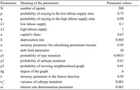
Table 2. Baseline parameters
Parameters Meaning of the parameters Parameter values
N number of agents 200
p probability of staying in the low labour supply state 0.75 q probability of staying in the high labour supply state 0.98
L1 low labour supply 0.1
L2 high labour supply 1
α capital’s share 0.67
δ depreciation rate 0.005
σ memory parameter for calculating permanent income 0.95
κ debt limit parameter 30
ρ1 probability of type mutation 0.0033
ρ2 probability of subtype mutation 0.01
ρ3 probability of rewiring neighbourhood graph 0.01
dg degree of the graph 6
λ memory parameter in the fitness function 0.95
ση2 variance of subtype mutation 0.001
ω interest rate determination parameter 0.001
Ergodicity rarely arises as a problem in economics. In practical terms station- arity implies that two distant observations on the same realization of a time series are almost independent. Thus tests for stationarity are most reliable when one has long observed time series, i.e. “large” samples. In addition, ergodicity means that all realizations are alike, while the lack of ergodicity implies that different reali- zations may behave qualitatively differently. Empirical economists can observe one realization of a time series, and though they have trust in the “largeness”
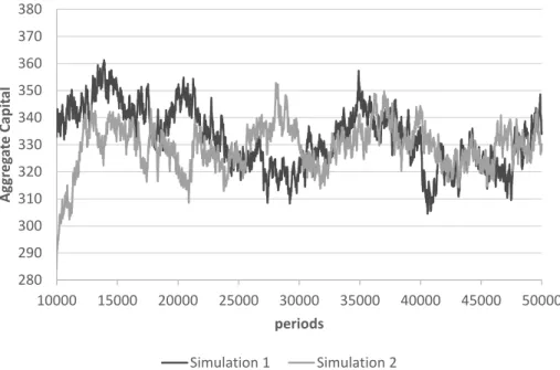
of their samples, they cannot distinguish between ergodicity and stationarity, as the distinction could be detected only if multiple realizations were available. Of course, with a simulation model one has the opportunity to test for both of these properties, as generating large samples and multiple runs with the same parame- ter values (and initial conditions) are feasible. As one can see in Figures 1 to 4 the trajectories of aggregate capital strongly suggest that our model is non-ergodic for the baseline parameterization, and stationarity is also questionable, judging by visual inspection.
Figure 1. The trajectories of aggregate capital in case of Γ = 0.0001 Source: authors
280 290 300 310 320 330 340 350 360 370 380
10000 15000 20000 25000 30000 35000 40000 45000 50000
AggregateCapital
periods
Simulation1 Simulation2
250
270 290 310 330 350 370 390
10000 15000 20000 25000 30000 35000 40000 45000 50000
Aggregate Capital
periods
Simulation 1 Simulation 2
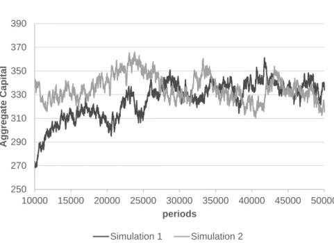
Figure 2. The trajectories of aggregate capital in case Γ = 0.001 Source: authors
300
310 320 330 340 350 360 370 380
10000 15000 20000 25000 30000 35000 40000 45000 50000
AggregateCapital
periods
Simulation1 Simulation2
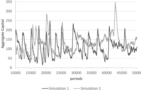
Figure 3. The trajectories of aggregate capital in case of Γ = 0.01 Source: authors
0
50 100 150 200 250 300 350
10000 15000 20000 25000 30000 35000 40000 45000 50000
AggregateCapital
periods
Simulation1 Simulation2
Figure 4. The trajectories of aggregate capital in case of Γ = 0.1 Source: authors
0
20 40 60 80 100 120 140
10000 15000 20000 25000 30000 35000 40000 45000 50000
AggregateCapital
periods
Simulation1 Simulation2
Figure 5. The trajectories of aggregate capital in case of Γ = 1 Source: authors
0
20 40 60 80 100 120 140
10000 15000 20000 25000 30000 35000 40000 45000 50000
AggregateCapital
periods
Simulation1 Simulation2
Figure 6. The trajectories of aggregate capital in case of Γ = 10 Source: authors
40 50 60 70 80 90 100 110 120 130 140
10000 15000 20000 25000 30000 35000 40000 45000 50000
AggregateCapital
periods
Simulation1 Simulation2
Figure 7. The trajectories of aggregate capital in case of Γ = 100 Source: authors
4.1.1. Testing for stationarity and ergodicity Parametric tests
Firstly, we performed the augmented Dickey-Fuller test (the most commonly used parametric test, when the null is non-stationarity (unit-root)), on the capital stock time series with different Γ (“temperature”) values (see Table 3). The optimal lag structure of the model was determined according to the Akaike information crite- rion. As Table 3 shows, for each Γ the null hypothesis of a unit root is rejected at conventional significance levels.
Table 3. Results of the Augmented Dickey-Fuller test in case of different Γ values Γ values 0.0001 0.001 0.01 0.1 1 10 100 1000000 MacKinnon
p-values 0.0006 0.0000 0.0113 0.0005 0.0000 0.0000 0.0000 0.0000 Source: authors
40 50 60 70 80 90 100 110 120 130 140
10000 15000 20000 25000 30000 35000 40000 45000 50000
AggregateCapital
periods
Simulation1 Simulation2
Figure 8. The trajectories of aggregate capital in case of Γ = 100000 Source: authors
Non-parametric tests
As the null hypothesis of the Dickey-Fuller test is rather specific, we looked for nonparametric tests, too. In any case it was necessary to conduct a test for ergo- dicity, and there exist fundamentally similar testing procedures applicable to both problems (Gibbons 1985). We opted for a methodology that has been applied to agent-based models, and is an application of the extension of the Wald-Wolfowitz test (Wald – Wolfovitz 1940) by Grazzini (2012).
The Wald-Wolfowitz (“runs”) test checks whether two samples come from the same distribution. Its extension by Grazzini tests whether a function fits well some set of observations, by noticing that the observations should be randomly distributed above and below the function, regardless of the distribution of errors.
Given the estimated function, 1 is assigned to the observations above the fitted line, and 0 to the observations below the fitted line. The statistics used to test the null hypothesis is the number of runs, where a run is defined as “a succession of one or more identical symbols which are followed and preceded by a different symbol or no symbol at all” (Gibbons 1985). The number of runs, i.e. too many or too few runs, may reflect the existence of non-randomness in the sequence. The null-hypothesis is that a given set of observations is randomly distributed around a given function.
In order to check whether the mean is stationary, a model was simulated for 50,500 periods, and this long series was divided into 100 windows, after dropping the first 500 observations. For each window the mean was computed, and it was checked whether the means of the subsamples were above or below the mean of the whole time series (the function whose “fit” we tested) by performing the Runs Test in its form with a two-sided alternative (see Grazzini 2012). Had the sub-sample means been randomly distributed around the overall mean, we would have concluded that the hypothesis of stationarity for the first moment cannot be rejected. As for all Γs the p-values were practically zeros, the null hypothesis of stationarity was flatly rejected. Thus the parametric test (with non-stationarity as the null), and the non-parametric tests (with stationarity as the null) provided contradictory answers.
To test the ergodic property, the runs test was used again, but in its original form, proposed in Wald – Wolfovitz (1940). The first steps of the ergodicity test are similar to the stationarity test: again a 50,500 periods long time series was simulated, then, after dropping the first 500 observations, it was divided into 100 windows, and the mean in each window was computed. The first sample of the test is formed by the means of the 100 sub-samples. As a second step, 100 time series of 1000-period length were generated with different random seeds, and the means were computed for each one, after dropping the first 500 values. The
second sample for the ergodicity test consisted of these 100 sample means. We merged them, and created a set which sorts the elements of these two sets into one of ascending order. Then the runs test was applied, where under the null hypoth- esis (ergodicity) the two samples had the same mean (see Grazzini 2012). For every value of Γ the p-values were again very close to zero, so the null hypothesis of ergodicity was in each case definitely rejected.
4.1.2. Interpretation
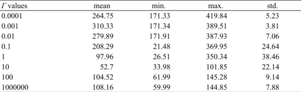
What is the content of non-ergodicity? Any ergodic process is such that differ- ent realizations of the process are essentially the same, thus one can discover the properties of a process from a single (long enough) realization as well as from an infinity (in practice a very large number) of different realizations. Stationar- ity but non-ergodicity means that we have to carry out many simulations with the same parameters, and computing statistics therefrom (ensemble averaging) to estimate the characteristics of the time series. In principle this averaging is appropriate only when stationarity prevails, but inappropriate when even station- arity is amiss. As we have seen we can have serious doubts even with respect to stationarity. Does it mean that calculating ensemble averages would be meaning- less? We believe that it is not necessarily the case, and Table 4, summarizing our results for the baseline parameterization, appears to justify this claim. In this table we report the mean, the minimum, and the maximum of the average capital stock and the average relative standard deviation for different values of the “tempera- ture” parameter. It can be seen that the numbers are not totally arbitrary, there are clear differences attributable to varying selection pressure. This statement is true not only for the mean but also for the ranges. Therefore we feel vindicated that reasonable conclusions can be drawn from following tables.
4.2. Main fi ndings
For any given parameter setting we ran 100 simulations, in each case for 5000 periods. For every run we dropped the first 3000 periods to eliminate any effects stemming from the assumptions that we used for starting the simulation, and cal- culated all statistics on the basis of the last 2000 simulated “observations” only.
The crucial observations concern the dependence of the capital stock on Γ (re- minder: low gamma amounts to high selection pressure.) One can see that very strong selection pressure tends to result in substantial over-accumulation, where the capital stock is, on average, much higher than its Golden Rule value. Though there are significant differences across runs (the symptom of non-ergodicity or non-stationarity) the ensemble average of capital is close to the Golden Rule
value, when selection pressure across types is very low (high Γ ). There seems to be an interesting non-linearity: at medium levels of Γ there tends to be under- accumulation, and the transition from under- to over-accumulation is not smooth, wildly different average capital stocks are realized for Γs in that parameter range.
The last column indicates that the relative standard deviation is smaller for lower gammas, thus the capital accumulation process seems to be more stable when the selection pressure is high.
Table 5 corresponds to Table 4, but with aggregate consumption replacing capital. The aggregate consumption figures in Table 5, reflect, of course, the evo- lution of the capital stock. The smaller ranges of average consumption are due to the concavity and non-monotonicity of the relationship between capital and consumption. On the other hand, the relative standard deviations are larger, thus consumption is more volatile within each run than capital. This is not surprising in itself, since capital is a stock, while consumption is a flow variable. What is interesting, however, is that low gammas now point to higher volatility (see the last column in Table 5), in contradistinction to the case of capital. Comparing Tables 4 and 5 one can observe that over-accumulation is more harmful than under-accumulation in terms of average consumption.
These findings together may constitute a puzzle. Naive evolutionists may be- lieve that letting evolution establish “preferences” of individuals would conduce to a socially “optimal” state, as the golden rule consumption is certainly very close to our intuition about social optimality.3
3 However, as an anonymous referee has pointed out, evolutionary forces can lead to free rid- ing phenomena as Vriend (2000), Vallée and Yildizoglu (2009) and Salle et al. (2017) have demonstrated.
Table 4. The mean, the maximum and the minimum of the average aggregate capital as a percentage of the Golden Rule capital, and the average relative standard deviation
of the aggregate capital (%) with different Γ values
Γ values mean min. max. std.
0.0001 264.75 171.33 419.84 5.23
0.001 310.33 171.34 389.51 3.81
0.01 279.89 171.91 387.93 7.06
0.1 208.29 21.48 369.95 24.64
1 97.96 26.51 350.34 38.46
10 52.7 33.98 101.85 22.14
100 104.52 61.99 145.28 9.14
1000000 108.16 59.99 144.85 7.88
Source: authors
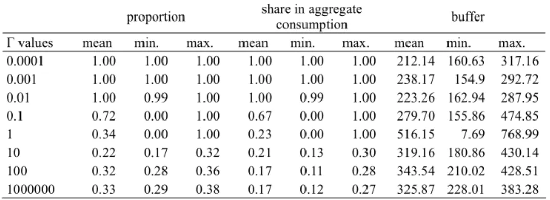
To understand why increasing selection pressure may cause harm to society we have to look at the fate of the different types. In Tables 6 to 8, statistics for buffer-stock savers, myopics, and permanent-income households are reported, respectively.
Columns (1) of Tables 6 to 8 provide a proximate explanation. At very low Γs buffer stock savers (prudent agents) dominate, but as the evolutionary pressure is reduced, myopics survive in more and more substantial numbers, and finally, at low selection pressure, the distribution of the three types, as expected, be- comes roughly equal in the long term. These observations suggest a rather clear viability ranking: 1. prudent, 2. myopic, 3, permanent-income. The proximate
“explanation” of the puzzle seems to work like this: when selection pressure is
Table 5. The mean, the maximum and the minimum of the average aggregate consumption as a percentage of the Golden Rule consumption, and the average relative standard deviation
of the aggregate consumption (%) with different Γ values
Γ values mean min. max. std.
0.0001 73.83 33.51 93.97 32.24
0.001 62.78 41.7 93.1 34.17
0.01 69.75 42.51 94.47 37.16
0.1 76.51 32.93 104.04 32.95
1 92.57 53.04 102.14 38.49
10 93.7 87.39 100.29 15.98
100 99.68 96.94 101.9 15.62
1000000 99.46 96.18 101.9 14.7
Source: authors
Table 6. Average proportion, average share in aggregate consumption and average buffer stock of the prudent type: mean, minimum and maximum of the mean in simulations
with different Γ values
proportion share in aggregate
consumption buffer
Γ values mean min. max. mean min. max. mean min. max.
0.0001 1.00 1.00 1.00 1.00 1.00 1.00 212.14 160.63 317.16
0.001 1.00 1.00 1.00 1.00 1.00 1.00 238.17 154.9 292.72
0.01 1.00 0.99 1.00 1.00 0.99 1.00 223.26 162.94 287.95
0.1 0.72 0.00 1.00 0.67 0.00 1.00 279.70 155.86 474.85
1 0.34 0.00 1.00 0.23 0.00 1.00 516.15 7.69 768.99
10 0.22 0.17 0.32 0.21 0.13 0.30 319.16 180.86 430.14
100 0.32 0.28 0.36 0.17 0.11 0.28 343.54 210.02 428.51
1000000 0.33 0.29 0.38 0.17 0.12 0.27 325.87 228.01 383.28
Source: authors
high, prudent households drive out myopic and more risk tolerant agents, but they behave with excessive caution, making harm to each other eventually.
We can gain further insight if we look at Column (3) in Table 6. The average buffer is lower the more buffer-stock savers dominate. Thus they are more cautious when have “rivals” among other types than when they compete only among them- selves at high selection pressure. With low selection pressure not only target capital buffers get higher, but they become rather diffuse (see the large range for high Γ in Column (3) Table 6). Inspecting column (2) in Tables 7 and 8 shows a curious situ-
Table 7. Average proportion, average share in aggregate consumption and average optimism of the permanent-income type: mean, minimum and maximum of the mean in simulations
with different Γ values
proportion share in aggregate
consumption optimism
Γ values mean min. max. mean min. max. mean min. max.
0.0001 0.00 0.00 0.00 0.00 0.00 0.00 - - -
0.001 0.00 0.00 0.00 0.00 0.00 0.00 - - -
0.01 0.00 0.00 0.00 0.00 0.00 0.00 - - -
0.1 0.00 0.00 1.00 0.04 0.00 1.00 0.96 0.82 1.09
1 0.03 0.00 0.87 0.04 0.00 0.89 0.92 0.86 0.99
10 0.09 0.03 0.45 0.09 0.03 0.45 1.05 0.8 1.25
100 0.29 0.25 0.33 0.32 0.27 0.37 1.27 1.06 1.53
1000000 0.33 0.29 0.37 0.38 0.32 0.43 1.3 1.11 1.48
Source: authors
Table 8. Average proportion, average share in aggregate consumption and average consumption drive of the myopic type: mean, minimum and maximum of the mean in simulations
with different Γ values
proportion share in aggregate
consumption optimism
Γ values mean min. max. mean min. max. mean min. max.
0.0001 0.00 0.00 0.00 0.00 0.00 0.00 – – –
0.001 0.00 0.00 0.00 0.00 0.00 0.00 – – –
0.01 0.00 0.00 0.00 0.00 0.00 0.00 – – –
0.1 0.24 0.00 0.83 0.28 0.00 0.87 1.04 0.86 1.18
1 0.00 0.62 0.95 0.73 0.00 0.95 1.03 0.83 1.18
10 0.68 0.35 0.77 0.70 0.35 0.82 1.01 0.89 1.12
100 0.39 0.34 0.44 0.51 0.40 0.61 1.04 0.90 1.21
1000000 0.34 0.30 0.38 0.45 0.36 0.52 1.02 0.90 1.18
Source: authors
ation: whenever other types survive they consume (per capita) more than prudent savers, making the latter de facto benefactors of others, at their own expense.
The basic mechanism can be explained as follows. In our economy with indi- vidual labour supply uncertainty, prudence is a valuable attribute. Those agents who have substantial wealth “buffers” can survive bad times, when their labour income is low, with little reduction in consumption. Myopic and permanent in- come agents must reduce consumption substantially when they are hit with nega- tive labour income shocks, even when borrowing is possible. With very high selection pressure, when only the fittest can survive, it leads to the disappearance of these types. On the other hand, prudence, though individually useful, results in over-accumulation, since aggregate labour supply uncertainty is almost nil. Thus high selection pressure creates a society of thrifty households with high wealth but negative capital income, who cannot even lend to others because they all be- long to the same prudent type. In other words, it is a society of misers who cause harm to each other by over-accumulating capital.
Suppose now that other types are introduced and selection pressure lessens, thus even those agents who have temporary loss of labour income, and there- fore largely reduced consumption, can survive. These people are less willing to accumulate wealth, and can even assume debt. Though individually they may go “hungry”, as a group, and in the long run, they consume more than misers since they have high labour income (capital is close to, and frequently above, the Golden Rule level), and interest rates are close to zero, since the net return on capital is also close to zero, and frequently negative. Thus in this economy crickets have roughly the same income as ants, but can consume more in the long run. If this seems counterintuitive, please notice that in our economy crickets and ants are exactly alike in the labour market, thus their labour income, in the long run, is the same. However, if there is too much capital then capital income is negative, therefore the usual assumption of “higher wealth earns higher income”
does not hold.
From the point of view of evaluating our approach to “endogenous prefer- ences” it is important to notice that the auxiliary parameters of the permanent- income and myopic types behave reasonably. Column (4) in Tables 7 and 8 shows the outcomes with respect to these. Concerning permanent-income households their optimism is definitely higher when the selection pressure across types is low. Quite “rationally” they tend to exploit prudent households by forming more optimistic pictures of the future, and therefore increasing consumption. On the other hand the consumption-drive of myopics is almost non-biased, irrespective of selection pressure.
5. CONCLUSIONS
In this paper we addressed two interrelated problems. First, can we set up a mac- ro-model focusing on savings without the assumption of utility maximization, but still preserving certain “rational” aspects of human decision making? Second, In this framework can we derive something interesting about long-run capital accu- mulation? Into a quite traditional production-primary income distribution frame- work we introduced consumption-types as embodiments of saving-functions akin to saving-functions popular in the traditional literature, and whose characteristics have been given some confirmatory evidence. These saving-functions evolve en- dogenously in our model due to evolutionary forces (selection and mutation). We have argued throughout this paper that this model is a possible solution to the first problem, though in no case the only one. We think that the stochastic properties of our model (non-ergodicity) are in its favour, despite the fact that these properties traditionally disqualify a macroeconomic model. It is obvious also that without a positive answer to the second problem this may turn out to be a rather shallow solution.
We believe that the model has provided us with interesting insights about capi- tal accumulation. It tells us that “ecologically rational” risk-aversion may turn out to be exaggerated from the social point of view, and it happens exactly when the fight for survival is intense. It means that lowering evolutionary pressure, resulting in more diversity in saver types, may be socially beneficial. Crickets may be, unintentionally, useful for society as a whole, including for prudent and cautious ants.
REFERENCES
Aiyagari, S. R. (1994): Uninsured Idiosyncratic Risk and Aggregate Saving. Quarterly Journal of Economics 109(3) :659–684.
Akerlof, G. A. – Shiller, R. J. (2010): Animal Spirits: How Human Psychology Drives the Economy, and Why It Matters for Global Capitalism. Princeton: Princeton University Press.
Banerjee, A. V. – Dufl o, E. (2011): Poor Economics: A Radical Rethinking of the Way to Fight Global Poverty. New York: Public Affairs.
Blanchard, O. J – Fischer, S (1989): Lectures on Macroeconomics. Cambridge, MA: MIT Press.
Blinder, P. (2005): Erdős – Rényi Random Graph. MATLAB Central File Exchange. https://
www.mathworks.com/matlabcentral/fi leexchange/4206-erdos-renyi-random-graph/content/
erdosRenyi.m, accessed 10/05/2015.
Carroll, C. D. (1997): Buffer-Stock Saving and the Life Cycle/Permanent Income Hypothesis. The Quarterly Journal of Economics 112(1): 1–55.
Carroll, C. D. – Summers, L. H. (1991): Consumption Growth Parallels Income Growth: Some New Evidence. In: Bernheim, B. D. – Shoven, J. B. (eds): National Saving and Economic Per- formance. Chicago: University of Chicago Press, pp 305–348.
Dobrescu, L. I. – Kotlikoff, L. J. – Motta, A. (2012): Why Aren’t Developed Countries Saving?
European Economic Review 56(6): 1261–1275.
Erdős, P. – Rényi, A. (1959): On Random Graphs. Publicationes Mathematicae 6: 290–297.
Fisher, I. (1930): The Theory of Interest. New York: Macmillan.
Fudenberg, D. – Levine, D. K. (2006): A Dual Self Model of Impulse Control. American Economic Review 96: 1449–1476.
Gibbons, J. D. (1985): Nonparametric Statistical Inference, 2nd ed. New York: Marcel Dekker Inc.
Grazzini, J. (2012): Analysis of the Emergent Properties: Stationarity and Ergodicity. Journal of Artifi cial Societies and Social Simulation 15(2): 7.
Hall, R. E. – Mishkin, F. S. (1982): The Sensitivity of Consumption to Transitory Income: Esti- mates from Panel Data on Households. Econometrica 50(2): 461–481.
Laibson, D. (1997): Golden Eggs and Hyperbolic Discounting. Quarterly Journal of Economics 112(2): 443–477.
Ljungqvist, L. – Sargent, T. J. (2004): Recursive Macroeconomic Theory, 2nd ed. Cambridge, MA:
MIT Press.
Piketty, T. (2014): Capital in the Twenty-First Century. Cambridge, MA: Harvard University Press.
Salle, I. – Yildizoglu, M. – Zumpe, M. – Sénégas, M. A. (2017): Coordination through Social Learning in a General Equilibrium Model. Journal of Economic Behaviour and Organization 141: 64–82.
Seppecher, P. – Salle, I. (2015): Deleveraging Crises and Deep Recessions: A Behavioural Ap- proach. Applied Economics 47(34-35): 3771–3790.
Vallée, T. M. – Yildizoglu, M. (2009): Convergence in the Finite Cournot Oligopoly with Social and Individual Learning. Journal of Economic Behavior and Organization 72(2): 670–690.
Vriend, N. J. (2000): An Illustration of the Essential Difference between Individual and Social Learning, and Its Consequences for Computational Analyses. Journal of Economic Dynamics and Control 24(1): 1–19.
Wald, A. – Wolfowitz, J. (1940): On a Test whether Two Samples Are from the Same Population.
The Annals of Mathematical Statistics 11(2): 147–162.
Open Access. This is an open-access article distributed under the terms of the Creative Commons Attribution 4.0 International License (https://creativecommons.org/licenses/
by/4.0), which permits unrestricted use, distribution, and reproduction in any medium, provided the original author and source are credited, a link to the CC License is provided, and changes – if any – are indicated. (SID_1)