Correspondence Between Vegetation Patterns and Soils in Wet and Wet-mesic Grasslands of Hanság and Tóköz
(Hungary)
Győző H
ASZONITS*– Dávid H
EILIGInstitute of Environmental Protection and Natural Conservation, University of Sopron, Sopron, Hungary
Abstract – Our research focused on the causes responsible for the fine mosaic pattern of plant associations on wet and wet-mesic meadows. The study area is located in the Little Hungarian Plain, including the former swamp basins of Hanság and Tóköz in Hungary. The vegetation survey data were evaluated by statistical methods (TWINSPAN method), and vegetation maps of the areas were prepared. Topsoil samples near the relevés were gathered for further laboratory tests. Soil profiles were opened by a Pürckhauer soil sampler for on-site description of the soil horizons and classification. Surface models provided a base for the preparation of contour maps that could be compared with the vegetation pattern. We found that of the two dominant vegetation types, mesotrophic wet meadows were associated with Mollic Gleysols, while non-tussock sedge beds were associated with Histic Gleysols. At the transitions of the two soil classes, the subgroup of non-tussock sedge beds is the dominant type. The soil class only determined the plant association on a habitat level, but it could not reason the fine pattern of the plant communities on the same soil class.
Canonical correspondence analysis (CCA) was performed to investigate the relationship between the distribution of dominant species and soil parameters. Several soil parameters combined have a significant effect on the distribution of dominant species. In conclusion, we found that the formation of association types strongly depends on the soil characteristics of the area, and that it is closely related to it. However, in the formation of the fine mosaic pattern, the driving ecological factors are the microrelief and the length of the saturated or flooded soil conditions.
phytocoenology / soil factors / soil-plant relationships
Kivonat – Összefüggés a vegetációmintázat és talajok között nedves és üde-nedves gyeptársulásokon a Hanság és Tóköz területén (Magyarország). Kutatásunk a nedves rétek fitocönózisanak, finommozaikos mintázatáért felelős okok felderítésére irányult. A vizsgálatok a Kisalföld nagytájon, ezen belül a Tóközben és a Hanság egykori lápmedencéiben történtek, Magyarországon. A választott mintaterületeken cönológiai felméréseket végeztünk, melyek felvételi adatait statisztikai módszerekkel (TWINSPAN analízis) kiértékeltük. Elkészítettük a területek vegetációtérképeit. A kvadrátok közelében feltalajmintákat vettünk, melyeket laborvizsgálatoknak vetettünk alá, valamint Pürckhauer-féle szúróbotos mintavevő segítségével 1 méteres talajszelvényeket vettünk a talajtípusok helyszíni leírásához. Beszereztük a vizsgálati területek felületmodelljeit, melyekből szintvonalas térképeket generáltunk így a domborzati eltéréseket össze tudtuk vetni a növényzet mintázatával. Megállapítottuk, hogy a két meghatározó növényzettípus közül a mocsárrétek a típusos réti talajokhoz, míg a magassásrétek a lápos réti talajokhoz kötődnek. A két talajtípus átmenetein a magassásrétek alcsoportja a meghatározó típus. Kimutattuk, hogy a talajtípus csak
* Corresponding author: hasz.gjozo@gmail.com; H-9400 SOPRON, Bajcsy-Zs. u. 4, Hungary
élőhely szinten (láp-, magassás, mocsárrét) határozza meg a növényzetet, az asszociációk egymással kialakított finom mintázatáért nem felelős. Az azonos talajtípusokon kifejlődött eltérő növénytársulások hasonló képet mutattak, így a finom mintázat kialakulását nem magyarázzák.
Kanonikus korrespondencia analízissel (CCA) kerestük a domináns fajok elterjedésének és a talajtani adottságoknak a kapcsolatát. Megállapítottuk, hogy a több tényező együttesen alakítja a fajok elterjedését. Összegezve, a társulástípusok kialakulása erősen függ a terület talajtani viszonyaitól, azzal szoros kapcsolatban áll. Azonban a finommozaikos mintázat kialakulásában a mikrodomborzat változatossága és az ezzel együtt járó vízborítottság különbség mértéke lehet a meghatározó ökológiai faktor.
fitocönológia / talajtulajdonságok / talaj-növény kapcsolatok
1 INTRODUCTION
The plant communities and soils of wet and wet-mesic grasslands formed water-rich environments (Scott et al. 1998). The saturated soil conditions and periodical flooding are important factors in these habitats. The common soil classes are Histosols (marsh soils) and Gleysols (meadow soils). In wet habitats, Histosols are formed as organic material accumulates, which is the result of persistent water saturation, anaerobic soil conditions, and the slowed decomposition of plant debris (Stefanovits et al. 2010). Wet to mesic habitats are affected by unsaturated soil conditions for shorter or longer periods of time, and flooding rarely occurs. The topsoil is well aerated under more mesic conditions, while wetter conditions lead to the accumulation of organic matter in the form of muck.
The distribution of species and their biomass production are highly determined by soils (Janssens et al. 1998, Duranel et al. 2007, Seabloom et al. 2021), but plants also affect the soils. Several studies aimed to answer whether this dynamic relationship could be detected between soil properties and vegetation diversity, but the relationship of soils and vegetation pattern is not explained completely (Scott et al. 1989, Ma et al. 2021).
The species composition of wet grassland plant associations is ruled by the nutrient contents, but pH, organic carbon content (TOC), and soil bulk density (BD) also play important roles (Bedforf et al. 1999). Extremely low BD (< 0.25 g·cm-3) signifies histic conditions where the nutrient levels are generally low while there is a vast amount of TOC.
Higher BD informs us about the different porosity of the soil and about the different water regime. Low pH can indicate the limitation of nutrient uptake or toxic conditions, while slightly acidic or neutral values are seen under more aerated soil conditions (Ma et al. 2021).
Along the changes of O2 and redox gradients, Josselyn et al. (1990) and Pennington – Walters (2006) observed patterns in the composition of plant vegetation. Even soil microbial communities have a strong relation with soil conditions and vegetation characteristics (Li et al. 2021). Michener (1983) investigated catenas in the northeastern part of United States regarding the composition and diversity of plant associations. He discovered a close relationship between soil zonation and plant community patterns. Bartha et al. (1996) described the relationship of site parameters and plant associations in a meadow in Bozsok (Zsidó-rét). The geomorphology of the mesotrophic wet meadow involved in the research is diverse, and many associations are represented in the area accordingly. Bartha et al. (1996) found that the zonation of the vegetation closely followed the zonation of the habitat and of the soils. Rajkai (1978) reports on his research in the floodplain of the Szilas stream, in which he states that the water regime of the different soil classes is closely related to the species composition of the plant association developed on their surface. Microtopography was found to be an important organizing structure of vegetation pattern (Diamond et al. 2019). Diamond et al. (2020) even revealed a correlation between soil chemical properties and microtopography. These studies showed that plant associations and soil types, especially soil
chemical properties, and relief have a close relationship. Nevertheless, many blank spots remain.
Focusing on the plant communities of wet and wet-mesic grasslands, there are generally numerous associations which are mixtures of lowland or colline plant associations. They form stripe- or mosaic complexes with each other. Several different associations were found in the plains, especially on the wet and wet-mesic grasslands of Hanság and Tóköz. Zólyomi (1934) presented the plan associations and habitat of Hanság. Járai-Komlódi (1960) described the plant associations of south Hanság. Keszei – Takács (2008) completed an overview of north Hanság habitats.
Wetlands and wet grasslands are disappearing all over the world (Hu et al. 2017). In Hungary, the proportion of these habitats is in constant decline due to climate change and anthropogenic effects (Kovács 1957, Tasi et al. 2014). The longer and more frequent dry periods have been especially detrimental (Borhidi – Sánta 1999, Bartholy et al. 2011).
Grassland and meadows are usually grazed or mowed, but the danger of overuse is always present (Janisova et al. 2013, Swacha et al. 2018, Bíró et al. 2020). Recording the current state of these habitats is also an important motivation.
The plant associations of the research area exhibited a mosaic pattern. Our research aims to find the reasons behind the observed pattern. We wanted to answer the following research questions: (1) Does the plant association pattern follow the soil diversity of the research area?
(2) Is there any soil parameter or groups of parameters that show direct relationship with species composition? (3) Is there a relationship between the vegetation pattern and microrelief?
2 MATERIALS AND METHODS
2.1 Study area
The Hanság and Tóköz (Csorna plain) are plains formed by tectonic subsidence and subsequent refilling of the area. Non-runoff areas are common due to topography.
Groundwater is generally close to the surface. The variability of the microrelief can have a large influence on vegetation. According to the Köppen-Geiger classification, the region is characterised by a warm temperate, fully humid, and hot summer climate (Cfb). (Berki et al.
2019a, b). Between 1961 and 2010, the annual mean temperature was 10.2°C and the annual rainfall was 564 mm. June is the wettest month. The forest aridity index (FAI) is 6.70, indicating a forest climate class with Turkey oak and sessile oak (Führer et al. 2019a, b).
The treeless plant communities of the micro-regions are characterized by mesotrophic wet meadows, non-tussock tall-sedge beds, mesotrophic wet meadows, and their transition parts. There are also mesic hay meadows, uncharacteristic wetlands, uncharacteristic mesic grasslands, and uncharacteristic dry and semi-dry grasslands that have become uncharacteristic due to anthropogenic effects. Our research investigated relatively small (<
10ha) areas in which the current treeless plant associations show a high degree of mosaic pattern. The visible difference in species composition was obvious even in the flat meadows.
Depending on the location, the various treeless associations alternated in the form of stripe complexes or mosaic complexes. Closely related coenoses are also separated in most cases (based on physiognomy, species composition).
2.2 Methods of botanical survey and soil investigation
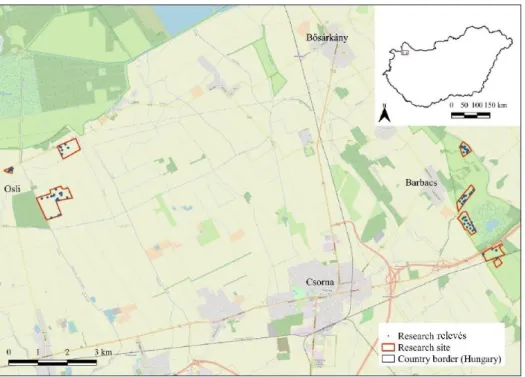
We conducted field surveys within the village boundaries of Barbacs and Osli in 2020 (Figure 1). The vegetation sampling is based on a modified Braun-Blanquet method – plant
cover percentage is used (Braun-Blanquet 1932). During the survey on the research area previously described, seven association types were searched and sampled. As a first step, satellite imagery was obtained and observed to delineate the plant community units. Then the field assessment, where the actual plant communities were identified and delineated, began.
Altogether 94 relevés were collected. In 21 relevés, topsoil sampling and description were also performed: three relevés from every plant association. The relevés were 5×5 meters. The location of the relevés was recorded by GPS-based point determination using a Trimble Geo XT field computer.
Figure 1. Map of the study area with the research sites and relevés
The nomenclature of plant species follows the work of Király (2009). We considered Borhidi’s (2003) work relevant in determining the associations. During the survey, we prepared a species list of the plants within the relevé and estimated the total cover, the percent of the open soil surface and the litter cover, and average vegetation height.
To determine the genetic soil type, we took soil profiles with a Pürckhauer sampler at the 21 selected relevés. The properties of genetic soil levels were recorded at the sites during the description. When naming soil types, we use both the Hungarian genetic system (Stefanovits 2010) and the nomenclature of the World Reference Base for Soil Resources (WRB) (FAO 2015). During field days, momentary soil moisture content (VWC) was measured at depths of 0-10 cm (VWC1), 10-20 cm (VWC2), and 20-30 cm (VWC3) (Aquaterr M-300) with three repetitions at every relevé. We took average soil samples from the upper 10 cm layer of the soil for laboratory tests on relevé level. Concurrently, 100 cm3 samples were also taken with sampling cylinders to calibrate the measured VWC and to measure the bulk density (BD).
2.3 Data processing, laboratory soil analysis and statistical testing
We classified the data collected during the vegetation survey into coenological tables. The coenological recordings were taken using the TURBOVEG database management software (Hennekens – Schaminée 2001), and then the statistical evaluation of the data was performed with the JUICE software package version 7.1 (Tichý 2002). The classification is based on the modified TWINSPAN method (Roleček et al. 2006). During the analysis, the maximum number of divisions was seven and the analysis was run using the average of the Simpson
index of dissimilarity as a measure of within-group heterogenity. The background information belonging to the formed groups (total cover (%), litter cover (%), etc.) come from the field observations. The diagnostic, constant, and dominant species of the established groups were defined following the method of Chytrý et al. (2002). The range of diagnostic species was determined by calculating the fidelity values based on the coefficient Φ. Fidelity values were calculated only for species that showed non-random occurrence across the clusters according to the Fisher’s exact test (P<0.05). The use of numerical vegetation classification aims to reduce the subjective factors of the expert-based classification. We give a brief summary of both classifications, but in the later analyses we use the vegetation groups based on the modified TWINSPAN analysis.
We performed laboratory testing of the soil samples based on the methodological recommendations of Bellér (2000) in the soil laboratory of the Institute of Environment and Earth Sciences of the University of Sopron. The undisturbed samples from the sampling cylinders were measured at the end of the field days and then dried at 105 °C for three days, after which they were measured again. In this way, we obtained VWC for calibration, and BD. The average or disturbed samples – collected near the cylinders – were dried at room temperature. After that, the skeletal parts, roots, and snail shells were removed from the samples. The pH (H2O) of the prepared soil samples was measured in a 1:2.5 soil:distilled water suspension (Motsara – Roy 2008). The determination of the ammonium-lactate-acetic acid soluble (AL) potassium and phosphorus contents is based on the methodology of Egnér et al. (1960), which showed the phosphorus (PAP) and potassium (PAK) contents that are available for the vegetation. Finally, the organic carbon content (TOC), and the total nitrogen (TN) and sulphur (TS) content of the soils were determined according to international standards (ISO 10694: 1995 and ISO 13878: 1998) using the Elementar Vario MAX CNS elemental analyser (Elementar Analysesysteme, Langenselbold, Germany).
We used a digital elevation model (DEM) from the Lechner Knowledge Centre called DDM-5 to visualize elevation, which was generated by digitizing 1:10000 scale topographic maps (Telbisz et al. 2013). Digitalization of the on-site drawn vegetation maps and visualization of the DEM was achieved by QGIS, version 3.18. Since elevation above sea level is not a good measure of microtopography in the present case – it provides no information about whether the given point is a bottom of a ditch or a top of a hummock – derived models are used to quantify the microrelief. The DEM is calculated into normalised elevation model and slope model. According to Diamond et al. (2019) hollows tend to have less-than-average elevation and less-than-average slope. This classification was compared with the manual delineation of hollows. The automated delineation has 14.6 % root mean square error (RMSE) against the manual one. At the level of TWINSPAN groups, the calculated values were compared to determine potential significant difference between them.
For this purpose, one-way analysis of variance (ANOVA) was applied with post-hoc Tukey- test.
R environment (R Core Team 2014) provided the further place for statistical analyses.
Pairwise correlation was calculated between soil parameters with Bonferroni-adjusted P values. Average values of the soil parameters were calculated at the level of the TWINSPAN groups. The soil parameters of the relevés assigned to the TWINSPAN groups were compered via ANOVA and homogenous groups were separated with Tukey’s honestly significant test.
To investigate the relationship between the soil parameters and the distribution of the dominant plants (cover percentages) among the TWINSPAN groups, canonical correspondence analysis (CCA) (Legendre – Legendre 2012, Oksanen et al. 2020) was applied. The soil parameters which showed high linear dependency were eliminated from the CCA; for this purpose both correlation analysis and calculation of variance inflation factor
(VIF) was performed. Variables which showed multicollinearity (VIF > 5) were left out from the CCA. Only tests with P < 0.05 are named as significant.
3 RESULTS
3.1 Results of the botanical survey
We investigated a total of seven association types in the study areas that were described in previous studies:
1. Glycerietum maximae Hueck 1931;
2. Galio palustris-Caricetum ripariae Bal.-Tul. et al. 1993;
3. Caricetum acutiformis Eggler 1933;
4. Caricetum gracilis Almquist 1929;
5. Caricetum distichae Steffen 1931;
6. Cirsio cani-Festucetum pratensis Májovsky – Ružičková 1975;
7. Carici vulpinae-Alopecuretum pratensis (Máthé – Kovács M. 1967) Soó 1971 corr.
Borhidi 1996;
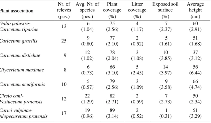
Table 1 introduces the average characteristics of the relevés on the plant association level.
Association types typically appear together in the form of stripe or mosaic complexes in the areas. They are well separated by their species composition and physiognomy, but usually there is a 1-8 m wide transition zone of adjacent associations where these associations are mixed. At gradually rising elevation, the associations follow each other in a stripe-like manner, while in flat areas they appear in patchy patterns.
Table 1. Average characteristics of the plant associations (mean (standard error of mean)) Plant association
Nr. of
relevés Avg. Nr. of species
Plant coverage
Litter coverage
Exposed soil surface
Average height
(pcs.) (pcs.) (%) (%) (%) (cm)
Galio palustris-
Caricetum ripariae 13 6
(1.04)
75 (2.56)
4 (1.17)
7 (2.37)
60 (2.91)
Caricetum gracilis 25 9
(0.80)
77 (2.10)
2 (0.52)
5 (1.61)
51 (1.68)
Caricetum distichae 9 12
(1.02)
78 (2.04)
3 (1.08)
10 (3.85)
37 (3.12)
Glycerietum maximae 8 6
(0.73)
66 (3.10)
5 (2.45)
14 (3.97)
56 (6.44) Caricetum acutiformis 10 5
(0.57)
79 (2.56)
3 (1.09)
9 (3.58)
66 (4.74) Cirsio cani-
Festucetum pratensis 12 22 (1.29)
82 (2.71)
2 (0.59)
7 (2.73)
50 (2.34) Carici vulpinae-
Alopecuretum pratensis 17 19 (0.96)
89 (3.14)
2 (0.52)
1 (0.31)
51 (3.29)
3.1.1 Vegetation of wet sites
The Glycerietum maximae association is typically associated with the marginal zone of watercourses, but it also appears in smaller hollows in wet meadows. Its species number is
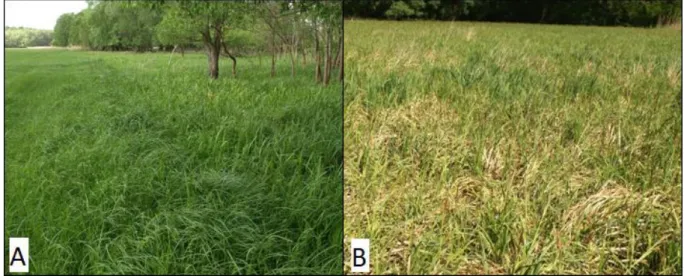
very low; the predominance of Glyceria maxima is obvious. The typical species are Symphytum officinale, Lythrum salicaria, and Ranunculus repens. As the habitat becomes drier, the Galio palustris-Caricetum ripariae association becomes dominant. The boundary between the two associations is usually marked by a sharp difference – transition happens in 1-2 m – due to the frequency of dominant species cover, which is usually characterized by a homogeneous carpet-like setting. In addition to the predominant Carex riparia, some constant elements are Lysimachia vulgaris, Persicaria amphibia, and Symphytum officinale. The Caricetum acutiformis association appears in almost identical habitats. The two associations differ most obviously in their dominant species; their appearance is similar. Moving away from the water, an association of Caricetum gracilis, which is more species-rich, more resistant to abiotic and biotic stress, is present. While the previous associations appear mostly as smaller spots or narrow stripes, these acute sedge associations are extensive. Their appearance is diverse, several compositions can be observed, from completely homogeneous acute sedge spots to broken-up, mosaic, and significantly more diverse settings. At some places, the Caricetum distichae association is wedged into the acute sedge associations as small spots and does not form large, connected stands. Typically, the patch area does not exceed 50 m2. The species diversity of both types of associations is moderate. In addition to Carex acuta, C. disticha, Cirsium brachycephalum, C. canum and Galium palustre are typical. Both types (4-5) are more resistant to mowing (i.e., cutting and removal of the cut biomass) than types 1-3. As a result of improper grassland management, associations 1-3 are easily transformed, most often into association type 4 (Figure 2 A), especially if types 1-3 are on edge habitats.
Figure 2. Effects of mowing (A) and accumulation of dry biomass on the soil surface (B)
The lack of grassland management makes the coenoses species-poor, mostly as a result of dry biomass accumulation (Figure 2 B), which makes many species unable to sprout. If sufficient water is available, the accumulation of sedge biomass is insignificant. However, this problem becomes common as the areas dry out.
3.1.2 Vegetation of wet-mesic sites
With the further decrease of the length of saturated periods, the dominance of sedge species also decreases; they are replaced by grass species. Typical associations in these areas are Cirsio cani-Festucetum pratensis and Carici vulpinae-Alopecuretum pratensis. Borhidi (2003) treats the association Carici vulpinae-Alopecuretum pratensis as a member of the Deschampsion caespitosae group. He mentions that the Ranunculo repentis-
Alopecuretum pratensis – which is poorer in Magnocarion species – is also closely related to it or that they are the same association. A more recent study sorts the Ranunculo repentis- Alopecuretum pratensis association into the Arrhenatherion group as a mesic-wet type (Lengyel et al. 2016). The most common habitats are colline and mountainous valleys. This association has a similar species composition as Carici vulpinae-Alopecuretum pratensis, but the proportion of the species of semi-dry grasslands and colline habitats is much higher.
Therefore, we identified the more water-tolerant associations of wet mesotrophic wet meadows as Carici vulpinae-Alopecuretum pratensis.
The former is a typical plant community of mesic habitats; the latter of wet-mesic habitats. In many cases, they connect to each other via broader (4-8 m) transition zones. Their species composition is characterized by the fact that they do not have typical character species. Dominant species are generalists with a wide range of tolerance, so in many cases it is difficult to appropriately differentiate these plant associations. Typical species of the Cirsio cani-Festucetum pratensis association include Festuca pratensis, Poa pratensis and Rumex acetosa. Its stands at the Hanság are more degraded; they lack rare species. The Carici vulpinae-Alopecuretum pratensis association is less disturbed, even Stellaria palustris appearing in its stand. Typical species are Alopecurus pratensis, Ranunculus acris, and Lathyrus pratensis.
3.2 Results of the modified TWINSPAN analysis
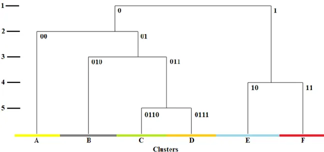
According to the analysis results, the investigated plant communities do not differ as much from each other as we identified in the field. Of the six clusters formed (Figure 3).
Figure 3. Modified TWINSPAN dendrogram of the 94 relevés
The first division brought the separation of the non-tussock tall-sedge beds (0) and the mesotrophic wet meadows (1). In the second division, the non-tussock tall-sedge beds (0) were divided into lesser groups: Caricetum gracilis × Caricetum distichae group (00) and a combination of Galio palustris-Caricetum ripariae group (01) This group (01) was divided into two subgroups: Caricetum acutiformis × Caricetum ripariae group (010) and the mixed group of Galio palustris-Caricetum ripariae associations (011). Group (011) collected the associations of wet and mesic habitats. This group is separated into two: the wet habitats were characterised by the Galio palustris-Caricetum ripariae × Glycerietum maximae group (0110)
and the wet-mesic habitats were populated by Galio palustris-Caricetum ripariae × Caricetum gracilis group (0111).
The division of mesotrophic wet meadows (1) partitions into two subgroups. Both subgroups have transient characteristics. Their separation is caused by the different moisture regimes; group (10) occurs under more wet conditions while group (11) prefers less wet conditions.
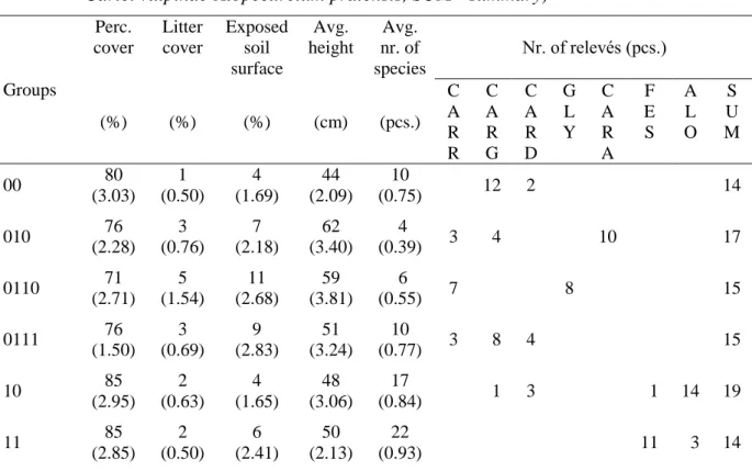
Table 2 summarises vegetation characteristics of the formed TWINSPAN groups and the distribution of relevés between the two classification systems. The detailed interpretation of the TWINSPAN groups is in the following subsections.
Table 2. Average vegetation characteristics of the TWINSPAN groups (mean (standard error of mean)) and the distribution of relevés between the plant associations and TWINSPAN groups (CARR - Galio palustris-Caricetum ripariae, CARG - Caricetum gracilis, CARD - Caricetum distichae, GLY -Glycerietum maximae, CARA - Caricetum acutiformis, FES - Cirsio cani-Festucetum pratensis, ALO - Carici vulpinae-Alopecuretum pratensis, SUM - summary)
Groups
Perc.
cover
Litter cover
Exposed soil surface
Avg.
height
Avg.
nr. of species
Nr. of relevés (pcs.)
(%) (%) (%) (cm) (pcs.)
C A R R
C A R G
C A R D
G L Y
C A R A
F E S
A L O
S U M
00 80
(3.03) 1 (0.50)
4 (1.69)
44 (2.09)
10
(0.75) 12 2 14
010 76
(2.28) 3 (0.76)
7 (2.18)
62 (3.40)
4
(0.39) 3 4 10 17
0110 71
(2.71) 5 (1.54)
11 (2.68)
59 (3.81)
6
(0.55) 7 8 15
0111 76
(1.50) 3 (0.69)
9 (2.83)
51 (3.24)
10
(0.77) 3 8 4 15
10 85
(2.95) 2 (0.63)
4 (1.65)
48 (3.06)
17
(0.84) 1 3 1 14 19
11 85
(2.85) 2 (0.50)
6 (2.41)
50 (2.13)
22
(0.93) 11 3 14
3.2.1 Caricetum gracilis × Caricetum distichae group (00)
This cluster shows a transitional character. The two associations usually form mosaic complexes with each other. Small patches (~50 m2) of Caricetum distichae are wedged into the carpet-like Caricetum gracilis stands. There is considerable overlap in species composition but there are differences in their dominant species and physiognomy.
Diagnostic species: Caltha palustris, Cardamine pratensis, Carex acuta, Carex vesicaria, Carex vulpina, Equisetum palustre, Lysimachia nummularia, Myosotis scorpioides, Persicaria dubia, Poa palustris, Ranunculus repens.
Constant species: Lychnis flos-cuculi, Rumex acetosa, Symphytum officinale, Taraxacum officinale.
Dominant species: Carex acuta, Carex disticha.
3.2.2 Caricetum acutiformis × Caricetum ripariae group (010)
This group is created from two plant associations which are easy to distinguish in the field.
However, both can be characterized as species-poor associations of hollows and wetter areas with a carpet-like setting. The associations share several species, and the physiognomy of the plant communities are determined by the dominant species. In most cases, Carex riparia and C. acutiformis are present together, but the dominant one has much higher cover percentage and more individuals. There is no evidence of codominance, which would imply the aggregation of the two associations. The TWINSPAN method aggregated these associations since their relevés were homogenous and since they have almost the same species with similar cover percentages. The difference is only shown in the dominant species (cover percentages).
Diagnostic species: Carex acutiformis, Lythrum salicaria.
Constant species: Carex riparia, Lysimachia vulgaris, Symphytum officinale.
Dominant species: Carex acutiformis, Carex riparia.
3.2.3 Galio palustris-Caricetum ripariae × Glycerietum maximae group (0110)
This is a transitional group of the wet areas. The group of mixed plant communities (0110) contains relevés of Galio palustris-Caricetum ripariae and Glycerietum maximae associations. This indicates that the assessment of differences between the investigated associations is not uniform. There is no significant difference in the species combination of the two types. However, the dominant species determines the appearance of the association, based on which they can be easily distinguished in the field. The program creates new groups based on the heterogeneity between the relevés. As these are quite similar based on their species composition, the analysis does not separate them into separate subgroups.
Diagnostic species: Carex riparia, Glyceria maxima, Persicaria amphibia, Schoenoplectus lacustris, Stachys palustris, Urtica dioica.
Constant species: Iris pseudacorus, Ranunculus repens, Symphytum officinale.
Dominant species: Carex riparia, Glyceria maxima.
3.2.4 Galio palustris-Caricetum ripariae × Caricetum gracilis group (0111)
This group is found in the transition zone of the wet and wet-mesic group. It is characterised by less wet conditions than in the case of 0110 group. These two groups often form stripe complexes or patch-complexes in micro-basins. Group 0111 is more species-rich than 0110 or the formerly introduced groups; however, it is more species poor than Caricetum gracilis. The species of the two associations mix equally and the two dominant species are often codominant.
Diagnostic species: Agrostis stolonifera, Carex acuta, Cirsium arvense, Cirsium brachycephalum, Galium palustre, Iris pseudacorus, Persicaria amphibia, Phalaris arundinacea, Symphytum officinale, Thalictrum flavum.
Constant species: Cardamine pratensis, Carex riparia, Lysimachia vulgaris, Ranunculus repens.
Dominant species: Carex acuta, Carex disticha, Carex riparia.
3.2.5 Carici vulpinae-Alopecuretum pratensis × Caricetum gracilis group (10)
This group of associations forms in the transition zone between mesotrophic wet meadows and non-tussock tall sedge beds and in the depressions of mesotrophic wet meadows. The presence of typical mesotrophic wet meadow species (Alopecurus pratensis, Cardamine pratensis, Galium mollugo) and an accumulation of aquatic species (Iris pseudacorus,
Phalaris arundinacea, Symphytum officinale) characterise the group. They are unstable plant communities, sensitive to changes in environment. The dominant species which is better adapted to the weather in a given year determines the community. They can experience significant change within a year.
Diagnostic species: Alopecurus pratensis, Calamagrostis epigeios, Cardamine pratensis, Carex hirta, Carex otrubae, Cerastium tenoreanum, Festuca pratensis, Galium mollugo, Glechoma hederacea, Lychnis flos-cuculi, Phalaris arundinacea, Poa pratensis, Potentilla anserina, Potentilla reptans, Ranunculus repens, Taraxacum officinale, Vicia cracca.
Constant species: Cirsium arvense, Cirsium canum, Iris pseudacorus, Symphytum officinale.
Dominant species: Alopecurus pratensis, Carex disticha, Festuca pratensis.
3.2.6 Carici vulpinae-Alopecuretum pratensis × Cirsio cani-Festucetum pratensis group (11)
The present cluster includes the typical mesotrophic wet meadows. In the absence of reliable character species, mesotrophic wet meadows are often difficult to distinguish from each other.
They occur in a fairly wide range of habitats due to their broad-spectrum generalist species, which define the community. The observed Cirsio cani-Festucetum pratensis association is more species-poor than described by Borhidi (2003). The stands of the Carici vulpinae- Alopecuretum pratensis association are mostly small, with a wide transition to the mesotrophic wet meadows dominated by Festuca species. Considering the above-mentioned facts, it is understandable that they were not separated in the analysis. Nevertheless, we consider their field isolation to be necessary because they indicate the changes in the water balance of the habitat.
Diagnostic species: Achillea millefolium, Anthoxanthum odoratum, Arrhenatherum elatius, Carex hirta, Carex praecox, Carex spicata, Cerastium brachypetalum, Cirsium canum, Colchicum autumnale, Dactylis glomerata, Daucus carota, Erigeron annuus, Festuca pratensis, Festuca rupicola, Fragaria viridis, Frangula alnus, Galium mollugo, Galium verum, Glechoma hederacea, Lathyrus tuberosus, Leontodon hispidus, Leucanthemum vulgare, Linaria vulgaris, Lotus corniculatus, Luzula campestris, Lychnis flos-cuculi, Myosotis arvensis, Myosotis ramosissima, Pastinaca sativa, Plantago lanceolata, Poa angustifolia, Poa pratensis, Potentilla reptans, Ranunculus acris, Rosa canina s.s., Rubus caesius, Rumex acetosa, Solidago gigantea, Veronica chamaedrys, Vicia hirsuta, Vicia tenuifolia.
Constant species: Alopecurus pratensis, Cirsium arvense, Potentilla anserina.
Dominant species: Alopecurus pratensis, Arrhenatherum elatius, Festuca pratensis.
3.3 Results of soil analyses
During the field investigations, we described hydromorphic soils with topsoil of different thickness and organic matter (OM) content. Mollic Gleysols (meadow soils) were found in three cases (more mesic parts of the wet-mesic habitats). In wet habitats Histic Gleysols (histic meadow soils) were more common, which were present in 12 relevés. Transient types of the two soil types were found in six cases in wet-mesic habitats, especially in which wet character dominates and it associates with only a lower accumulation of OM. These are described as Mollic Gleysol (Hyperhumic). These soils have looser topsoil and higher OM
content (muck layer) than the described Mollic Gleysols, but they do not reach the requirements of histic properties.
The correlations between the individual soil parameters demonstrated that elevation and pH (H2O) have no significant relationship with the other variables, except with each other (r = 0.47). All the other correlations proved to be significant. PAK shows a strong positive correlation (0.50 < r < 0.60) with PAP and TS, while it has a medium positive correlation with TN (r = 0.47) and a negative one with BD (r = -0.45). PAP is correlated strongly (r > 0.60) positively with TOC, TN, TS, VWC1, VWC2 and VWC3 and negatively with BD (r = -0.76).
TOC, TN, and TS have strong positive connection with each other (r > 0.95), and with the VWC too (r > 0.84). The relation of BD and TN, TS is described as strong negative (r < - 0.89). Between BD and the VWCs the connection strongly negative (r < -0.85). The group of moisture contents (VWC1, VWC2, VWC3) have correlation coefficients above 0.95 with each other, which indicates a strong positive relationship.
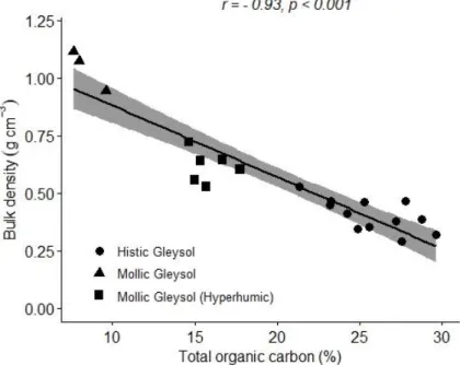
TOC and BD show a strong negative relationship (Figure 4) and the soil profiles of different classes cluster along these parameters. In the case of Mollic Gleysols, the lower TOC is associated with a high BD value, which indicates that the humic character does not dominate, but a relatively high, above 7%, TOC was observed as a result of OM accumulation. In the transitional group, TOC jumps, above 10%, but does not reach 20%. In parallel, BD decreases. As the histic character became predominant, a high TOC of over 20%
was measured as a result of organic matter accumulation, which is accompanied by a very low BD.
Figure 4. Relation of soil bulk density (BD) and total organic carbon (TOC) along different soil groups
3.4 Correlation between soil parameters and TWINSPAN groups
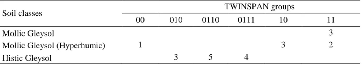
There is a correlation between the soil classes and the TWINSPAN groups (Table 2). On Mollic Gleysol, only group 11 can be found, while on Histic Gleysol, we typically find groups 010 and 0110, and group 0111. In the case of the transient Mollic Gleysol (Hyperhumic), the transient vegetation group 10 is predominant, but groups 00 and 11 also occur.
Table 2. Distribution of number of relevés among the TWINSPAN groups and soil classes
Soil classes TWINSPAN groups
00 010 0110 0111 10 11
Mollic Gleysol 3
Mollic Gleysol (Hyperhumic) 1 3 2
Histic Gleysol 3 5 4
The average soil parameters calculated for the TWINSPAN groups are presented in Table 3. Since group 00 has only one observation, it was omitted from the analyses and the values of that one relevé are presented in the table. Similarly to the classification by soil groups, there is no sharp separation between the individual TWINSPAN groups in terms of elevation, pH(H2O), and PAK. For PAP, TOC, TN, and TS parameters, the TWINSPAN groups are divided into two groups. 00, 010, 0110 and 0111 form a group dominated by the histic character, while groups 10 and 11 are found in the other group, where the meadow soil character predominates.
Table 3. Soil params of the different TWINSPAN groups (mean (standard error of mean))
Soil parameters TWINSPAN groups F Sign.
00 010 0110 0111 10 11
Nr. of elements
(relevés) (pcs.) 1 3 5 4 3 5
Elevation (m) 110 110a 109a 109a 110a 111.4a 1.31 NS
(0.000) (1.304) (0.408) (1.155) (0.678)
pH (H2O) 6.9 6.2a 6.4a 6.5a 6.5a 6.7a 0.87 NS
(0.082) (0.173) (0.225) (0.24) (0.094) Plant Available P
(mg 100 g-1)
16.2 18.3a 15.3a 14.7a 6.2b 5.3b 13.54 ***
(0.789) (2.286) (1.462) (0.681) (0.691) Plant Available K
(mg 100 g-1)
17.5 30.0a 24.6a 19.7a 14.9a 16.4a 2.38 NS (4.693) (5.55) (1.975) (1.187) (1.392)
Total Organic C (%) 15.7 27.3a 25.5a 25.0a 15.5b 11.7b 20.5 ***
(2.007) (1.17) (0.864) (0.633) (2.058)
Total N (%) 1.5 2.2a 2.2a 2.2a 1.4b 1.0b 18.65 ***
(0.132) (0.103) (0.037) (0.07) (0.18)
Total S (%) 0.3 0.6a 0.6a 0.5a 0.2b 0.2b 20.74 ***
(0.099) (0.035) (0.027) (0.021) (0.034) Bulk Density
(g cm-3) 0.5 0.4a
(0.042)
0.4a (0.044)
0.4a (0.019)
0.6ab (0.047)
0.9b (0.107)
10.22 ***
Water Content 62.5 86.9a 95.0a 98.9a 78.0a 45.3b 22.39 ***
0-10 cm (%) (8.613) (2.165) (0.634) (11.018) (3.062)
Water Content 63.9 82.4a 91.9a 96.9a 72.4a 43.3b 13.49 ***
10-20 cm (%) (9.88) (3.547) (1.835) (14.601) (3.266)
Water Content 59.9 86.1a 92.5a 96.9a 75.5a 44.5b 16.86 ***
20-30 cm (%) (8.612) (2.593) (1.545) (12.35) (4.058) Significance levels: 0 < *** ≤ 0.001 < ** ≤ 0.01 < * ≤ 0.05 < NS
abc represents homogenous subsets according to Tukey's honestly significant difference test
According to the BD of soils, the subsets are similar to the former case, but group 10 forms a transition and can be classified into both groups. Moisture contents show a uniform picture; only group 11 deviates from the other groups.
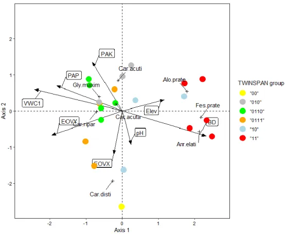
CCA was performed to show the correspondence of the main environmental factors with the composition of dominant plant species, (Figure 5). Soil and topographical variables were represented as arrows (eight altogether). Arrow length indicates the importance of the environmental variable. To avoid multicollinearity, variables showing higher variance inflation factors than five were omitted. The analysis was based on 21 relevés pictured by points and coloured according to their TWINSPAN group. The plant species were indicated by crosses. The location of the plant species relative to the arrows or axes represent the environmental conditions or gradients associated with the occurrence of the species.
The CCA model proved to be significant according to the permutation test (F = 1.748, P
= 0.004). The total inertia is 4.746 from which 53.8% was described by the constrained axes.
The first axis explained 18.4% of the total variation (34.2% of the constrained inertia), while the second axis covered 14.9% of the total inertia (27.6% of the constrained one). The coefficient of multiple determination (R2) is 0.538 and the adjusted coefficient of multiple determination (R2adj.) is 0.234. The species – environmental correlation is strong, r = 0.95 in the case of the Axis 1 and r = 0.89 for Axis 2.
Figure 5. Results of the Canonical Correspondence Analysis (CCA) between the soil parameters (arrows) and cover percentage of the dominant species of the TWINSPAN groups (crosses), points represent the relevés grouped by the TWINSPAN groups. Abbreviations:
Elev: Elevation (m), EOVY and EOVX: longitude and latitude in HD72 6 EOV reference system, pH: pH (H2O), PAP: Plant Available Phosporus (mg 100 g-1), PAK: Plant Available Potassium (mg 100 g-1), BD: Bulk Density (g cm-3), VWC: Volumetric Water Content of soil layer between 0 and 10 cm (%), Alo prate: Alopecurus pratensis, Arr. elati: Arrhenatherum elatius, Car acuta: Carex acuta, Car acuti: C. acutiformis, Car disti: C. disticha, Car ripar:
C. riparia, Fes prate: Festuca pratensis, Gly maxim: Glyceria maxima
The most important factors are BD, VWC, EOVY, PAP, and PAK. The first axis has a strong positive correlation with BD (r = 0.818) and strong negative with VWC1, EOVY, PAP (r = -0.856, -0.687, -0.639 respectively) and medium positive with elevation (r = 0.409). The second axis was affected mostly by PAK (r = 0.446) and medium negative correlation was shown with EOVX (r = -0.394) and pH (r = -0.305).
3.5 Results of vegetation mapping
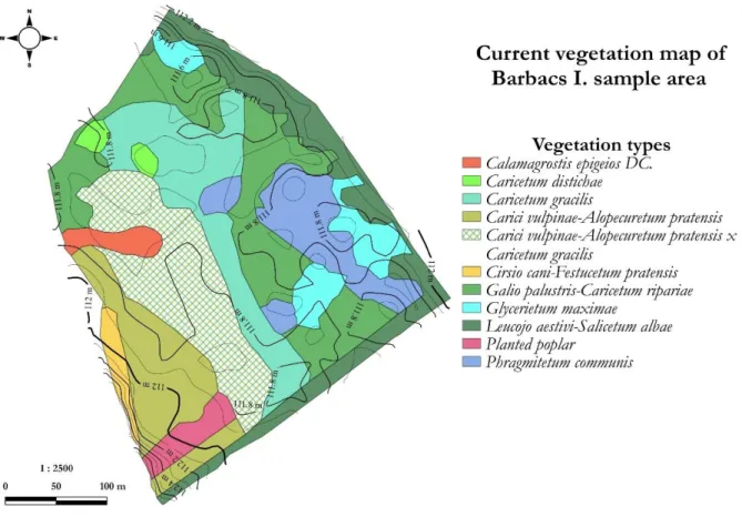
The reason for the fine mosaic pattern of vegetation formed in flat areas should also be investigated in the microrelief differences. Therefore, we fitted 5×5 m resolution digital elevation models to the study areas and made a comparison with the pattern of vegetation patches surveyed during vegetation mapping. The vegetation patches and the fine-scaled (10 cm increase in elevation) equiheight lines coincide in several cases (Figure 6).
Figure 6. Current vegetation map of Barbacs I. sample area
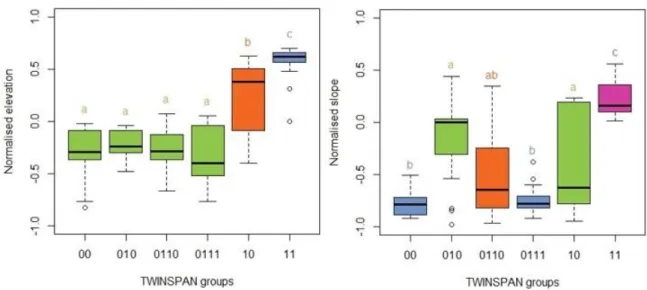
The normalised elevation values of the TWINSPAN groups differ significantly (F = 32.94, P < 0.001). There are three subsets separated by Tukey’s test. TWINSPAN group 00, 010, 0110, and 0111 are the ones which have average values lower than 0. Group 10 is a transient group and group 11 has the highest values and highest average. Normalised slope values show a different image. Significant difference among the groups is evident (F = 16.67, P < 0.001). The lowest values are accompanied with group 00 and 0111. Group 0110 shows a transition between subset a and b. Subset b (TWINSPAN group 010 and 10) are in the mid- range, while group 11 has again the highest average (Figure 7).
The TWINSPAN groups are assigned with the category of hummock or hollow according to the combined models of normalised elevation and slope on the level of relevés. The groups showed considerable differences (F = 18.04, P < 0.001). Tukey’s test divided the group into
two subsets. TWINSPAN group 00, 010, 0110, and 0110 are assigned to the hollow subset and TWINSPAN group 10 and 11 classified into the hummock subset. TWINSPAN group 00 has relevés only in hollows, 0110 and 0111 have three and one hummock relevés respectively while the rest of the relevés are hollows. TWINSPAN group 010 has five hummock and 12 hollow relevés, group 10 has a similar distribution but with swapped groups (13 hummocks and six hollows). Group 11 has only hummock relevés.
Figure 7. Normalised elevation and slope boxplots of the different TWINSPAN groups.
Groups with different colours are significantly different.
4 DISCUSSION
During the vegetation mapping and the more detailed investigation, we found the earlier mentioned seven (i.e., subsection 3.1) plant associations (Zólyomi 1934, Járai-Komlódi 1960, Keszei–Takács 2008). The recorded relevés went under a TWINSPAN analysis, which resulted in six association groups. These groups overlap; the numerical analysis aggregates closely-related plant communities e.g., Galio palustris–Caricetum ripariae × Glycerietum maximae (0110) group. These two associations differ only in the dominant species. Our assumption is that the TWINSPAN method lowers the subjectivity of the expert-based description, and it provides more reliable data for further analyses. Beside the TWINSPAN analysis, other methods could be used and compared to classify the relevés.
The soil survey revealed different forms of Gleysols, which is the typical soil class of wet and wet-mesic meadows. The soil groups differed in nutrient contents, BD values, and VWCs, but not in pH, elevation, and PAK. Similar results are presented by Heil et al. (2008), but they found significant difference between soil groups and pH values. This is also supported by Ma et al. (2021) and Li et al. (2017). The soil groups spread among the TWINSPAN groups following a water gradient. Soils with more moisture content were found under more water tolerant TWINSPAN groups. Li et al. (2017) reported similar findings. The difference of the soil parameters of the TWINSPAN groups followed a similar pattern as in the case of WRB soil groups, except PAP, which showed significant difference only among the plant community groups. P content was found to be an important factor in plant composition of a site in several studies (Bigelow – Canham 2002, Amorim – Batalha 2007, Hammersmark et al. 2009, Mellado – Zamora 2015, Onur – Suha 2016). The plant associations follow the changes of the soil classes, but the finer pattern of the plant composition is not explained by the soil groups (Research question 1). The higher number of relevés and the periodical returns
to the same relevés could represent a more detailed relationship between the soils and plant communities. This can also help the land managers to set the optimal timing of mowing or grazing, e. g. only after the seeding of protected species.
The distribution of relevés according to their dominant species are organised along two gradients. The first axis represents soil porosity or wet to dry gradient. This axis separates the relevés of hollows, ditches, and the ones which are located on relatively elevated places. The species on the positive end of Axis 1 are typical species of mesic meadows, while the species around the origin are found in wet meadows. Jager et al. (2015) and Li et al. (2017) found soil physical parameters crucial for the distribution of plant communities. The second axis shows a nutrient uptake gradient. Generally, the higher pH values – in this context it means neutral pH levels – accompany the sites where the nutrient uptake is not limited by acidic pH. The positive correlation of the PAP, PAK levels and Axis 2 along with a negative relation with pH (H2O) seems to be contradictious. The relevés affected by groundwater have lower pH values, which cause limited nutrient uptake, and the groundwater is usually richer in nutrients due to the fertilization of the adjacent arable lands. These processes can result in higher PAP, PAK or even TN levels than in relevés affected only rarely by groundwater. Species with higher nutrient needs occur on the negative end of this axis, while the positive values on this axis are accompanied by species which require lower nutrition levels. Groups of soil parameters show close relationship with the species composition of the study area, but soil physical parameters, therefore the water regime, seems to be a more fundamental factor than soil chemical characteristics (Research question 2). The larger number of relevés could result in a stronger connection between environmental and plan data.
The vegetation follows the changes in the microrelief of the sample areas (Figure 6 and Figure 7). Differences in elevation in these areas are small. Between the highest and lowest point of the total area the difference in elevation is only 1.4 m. Even on the fields, the vegetation follows the 10–20 cm height differences. Where the surface rises “suddenly”, the plant communities are arranged in stripes, and where the surface is nearly flat, they show a patchier arrangement. The analysis the DEM helped to make the correlation quantifiable between vegetation pattern and microtopography. Our findings support the results of Diamond et al. (2019) – as patch distribution is affected highly by the presence or by the lack of water. Some plant communities occur only in hollows and some are dry tolerant groups that were found on hummocks (Research question 3). Ladányi et al. (2016) described similar allocation of plant communities in a saline wetland. Future studies may use a higher spatial resolution DEM or even terrestrial laser scanning along with spatial statistics to find more fine-scaled relations.
Thus, it can be stated that the formation of different types of associations is highly dependent on the soil conditions of the area and can be closely related to it. However, in the formation of the fine mosaic pattern (in a lowland environment) the diversity of the microrelief and the differences in the period of flooding or saturated soil conditions play a crucial role (Jager et al. 2015, Li et al. 2017, Ma et al. 2021, Diamond et al. 2019, Diamond et al. 2020).
5. CONCLUSIONS
The present study examined the correlations between the characteristic soil types of the Hanság and Tóköz and the grassland plant associations that have developed on them. The soil classes of the sample areas and the physical and chemical properties of the topsoil were determined using laboratory tests. The plant associations of the areas and the microrelief categories produced from surface models showed close relationship. The patches of the
vegetation maps coincided with the hummock and hollows categories. The results of the plant association analysis were compared with the results of soil characteristics. We found that soil type determined the predominant vegetation type on a habitat level, but it is not responsible for the mosaic pattern formed by the associations. The distribution of the dominant species of the plant groups were closely determined by groups of soil parameters according to the CCA.
We also found that the microrelief changes, and therefore the length of the saturated or flooded soil conditions, can be the reason behind the mosaic pattern of the vegetation pattern.
According to our results, the vegetation follows the changes in the microtopography adequately, and it also indicates the minimal (10–20 cm) deviations reliably. Future studies should consider using more environmental parameters such as precipitation and groundwater fluctuation in multiple analyses.
Acknowledgements: Supported by the ÚNKP-20-3-II-29 New National Excellence Program of the Ministry for Innovation and Technology from the source of the National Research, Development and Innovation Fund.
REFERENCES
AMORIM, P. K. – BATALHA, M. A. (2007): Soil-vegetation relationships in hyperseasonal cerrado, seasonal cerrado, and wet grassland in Emas National Park (Central Brazil). Acta Oecologica 32:
319–327. https://doi.org/10.1016/j.actao.2007.06.003
BARTHA,D.–BIDLÓ,A.–KOVÁCS,G.–MARKOVICS,T. (1996): Termőhely és vegetáció kapcsolata a Bozsoki Zsidó-réten. [Interactions of site paramters and vegetation at the Zsidó-meadow at Bozsok (Hungary).] Erdészeti és Faipari tudományos Közlemények 40-41: 27–46. (in Hungarian) BARTHOLY, J. – BIHARI, Z. – HORÁNYI, A. – KRÜZSELYI, I. – LAKATOS, M. – PIECZKA, I. – PONGRÁCZ,R.–SZABÓ,P.–SZÉPSZÓ,G.–TORMA,CS.(2011):Hazai éghajlati tendenciák. In:
BARTHOLY,J.–BOZÓ,L.–HASZPRA,L. (ed.): Klímaváltozás-2011 / Klímaszcenáriók a Kárpát- medence térségére [Climate change–2011 / Climate scenarios of the Carpathian basin]. Magyar Tudományos Akadémia és az Eötvös Loránd Tudományegyetem Meteorológiai Tanszék, Budapest, pp: 145–169. (in Hungarian)
BEDFORD,B.L.–WALBRIDGE,M.R.–ALDOUS,A.(1999): Patterns in nutrient availability and plant diversity of temparate North American Wetlands. Ecology 80: 2151–2169.
https://doi.org/10.2307/176900
BELLÉR, P. (2000): Talajvizsgálati módszerek [Methods of soil analysis]. Nyugat-Magyarországi Egyetem Kiadó, Sopron. 107 pp. (in Hungarian)
BERKI, I. –BIDLÓ,A. – BÖLÖNI, J.– VIG, P. (2019a): 38.1.2. Természetföldrajzi jellemzés [38.1.2.
Geographical description]. In FÜHRER, E. (ed.): Magyarország erdészeti tájai. IV. Kisalföld erdészeti tájcsoport. [Forestry Region of Hungary IV. Kisalföld Forestry Region].
Agrárminisztérium Nemzeti Földügyi Központ, Budapest, Hungary, pp: 108-119 (in Hungarian) BERKI, I.– BIDLÓ, A.– BÖLÖNI, J.– VIG,P. (2019b): 39.1.2. Természetföldrajzi jellemzés [39.1.2.
Geographical description]. In FÜHRER, E. (ed.): Magyarország erdészeti tájai. IV. Kisalföld erdészeti tájcsoport. [Forestry Region of Hungary IV. Kisalföld Forestry Region].
Agrárminisztérium Nemzeti Földügyi Központ, Budapest, Hungary, pp: 184-198 (in Hungarian) BIGELOW,S.W.–CANHAM,C.D.(2002):Community organization of tree species along soil gradient
in a North-eastern USA forest. Journal of Ecology 90: 199–200. https://doi.org/10.1046/j.0022- 0477.2001.00655.x.
BÍRÓ,M.– MOLNÁR,ZS. –ÖLLERER,K.–LENGYEL,A.–ULICSNI,V. –SZABADOS,K.–KIŠ,A.– PERIĆ,R.–DEMETER,L. –BABAI,D(2020): Conservation a herding cobenefit from traditional extensive wetland grazing. Agriculture. Ecosystems and Environment 300: 106983 https://doi.org/10.1016/j.agee.2020.106983
BORHIDI, A. (2003): Magyarország növénytársulásai [Plant associations of Hungary]. Akadémiai Kiadó, Budapest. 569 pp. (in Hungarian)