Comparing the Reliability of Biomedical Texture Analysis Tools on Different Image Types
Monika Béresová
1*, Attila Forgács
2,3, Blanka Bujdosó
3, András Székely
4, József Varga
3, Ervin Berényi
1, László Balkay
31 Div. of Radiology, Department of Medical Imaging, Faculty of Medicine, University of Debrecen, Nagyerdei krt. 98, 4032 Debrecen, Hungary E-mail: beres.monika@med.unideb.hu; eberenyi@med.unideb.hu
2 Scanomed Nuclear Medicine Center, Nagyerdei krt. 98, 4032 Debrecen, Hungary; E-mail: forgacs.attila@scanomed.hu
3 Div. of Nuclear Medicine, Department of Medical Imaging, Faculty of Medicine, University of Debrecen, Nagyerdei krt. 98, 4032 Debrecen, Hungary
E-mail: bujdoso.blanka@kenezy.unideb.hu; jvarga@med.unideb.hu;
balkay.laszlo@med.unideb.hu
4 Kenézy Gyula Hospital, Department of Radiology, Bartók Béla út 2-26, 4031 Debrecen, Hungary; E-mail: andras.szekely@med.unideb.hu
Abstract: The aim of this study was to analyze the reliability of texture index (TI) calculations using two different approaches.
First, we calculated texture parameters on synthetically constructed images using four different biomedical software tools (CGITA, InterView Fusion, Matlab, MaZda). Second, we investigated the reliability of texture parameters, particularly how the texture indices diverge between two similar images with substantially different texture.
We generated five different heterogeneous synthetic images, thereafter, histogram-based and co-occurrence matrix features were calculated. The co-occurrence based indices were computed after two (8 and 64) different gray scale normalizations. For the reliability test, we compared 22 texture indices using a histological slice of the brain and Michelangelo's painting, and the gray level dependence was also analyzed.
The histogram-based parameters of all images and from all software were very similar.
Differences were found in the co-occurrence based indices after both gray level image normalizations. The reliability tests showed that from 22 parameters only 5 texture indices changed more than 20%, and at least 64 normalization levels were necessary for acceptable results. Our results underline that in medical multicenter studies it is especially critical to use the same software package. Some parameters do not reliably reflect changes, so texture analysis (TA) should be used with caution.
Keywords: texture analysis; medical imaging; software; comparative study; co-occurrence matrix
1 Introduction
There is an increasing interest in the use of medical imaging to describe tumor tissue characteristics. Radiomics is a new field that intends to capture more information (intensity histogram-based data, shape information, intra-tumor heterogeneity, special texture features) from the image of an organ [1]. Texture analysis (TA) was first introduced in MRI in the nineties [2] and is frequently used for analyzing and differentiating anatomical areas [3]. In addition, TA has become very common in all medical imaging modalities such as ultrasound (US), computed tomography (CT), magnetic resonance imaging (MRI), and positron emission tomography (PET) for the quantification of tumor heterogeneity. Several different methods exist for texture classification, such as statistical methods, filter- based techniques, model-based schemes, and structural approaches [4]. The first application was introduced by Haralick and Shanmugam; they used statistical feature characterization by computing the gray level co-occurrences matrix (GLCM). The co-occurrence matrix represents the relationship between intensity values in a given direction and distance in the image [5].
Despite several attempts to reveal the meaning of different TIs, we still do not fully understand, how the TIs should change when the texture of an image varies, nor how a different image texture could be associated with a TI range [6]. Further research in this topic could be crucial to establish the applicability of any TI in the biomedical area.
On the other hand, many techniques and software solutions have been proposed for the calculation of TIs. There are several software tools frequently used in the medical field such as MaZda [7, 8, 9], Matlab-based CGITA [10], the
“GLCM_textureToo” Java tool [11], the ImageJ “Texture Analyzer” plugin [12, 13, 14], several modules of the Matlab “Image Processing Toolbox” [15], TexRad [16], InterView Fusion [17], ABAQUS [18, 19] and FRAGSTATS [20], some of which are free.
MaZda is a special computer program for the calculation of several texture parameters from digitized or medical images. This package contains the B11 program (COST B11 European project) for texture analysis and visualization.
MaZda was used by Albuquerque et al. for texture analysis of damaged gray nuclei in amyotrophic lateral sclerosis; by Yan et al. to differentiate renal cell carcinoma, by Orphanidou-Vlachou et al. to quantify brain tumors; and by J MacKay et al. to study bone texture [21, 22, 23, 24].
Matlab is a scientific numerical computing environment and fourth-generation programming language with a wide range of toolboxes. Some frequently cited applications for texture analysis include CT texture analysis by Daginawala et al., the quantitative evaluation of skeletal muscle defects by Liu et al., and the texture analysis of brain MR images by Michoux et al. [25, 26, 27].
CGITA was developed under Matlab by Fang et al., originally used to quantify tumor heterogeneity in molecular images [10, 28]. InterView Fusion is a general- purpose multimodality medical image analysis software developed by Mediso Ltd.
It comprises a wide range of functions and special tools that provide detailed, fast and sophisticated evaluation of medical images [29].
Most research groups in this field use in-house software for computing tumor heterogeneity without demonstrating how the reliability of the software was tested [30, 31 32, 33, 34]. Since the algorithms that are used for heterogeneity index (HI) calculations are not always simple, the developed codes should be validated in some manner. In addition, there is no generally accepted concept on how to validate the different HI calculation software from various research groups and vendors. A solution to this issue might be if a collection of synthetic images, constructed with numerous, simple geometrical shapes such as rectangles and circles, were used to define heterogenic patterns, and then applied for software validation.
The aim of this study was to compare the texture analysis calculations of four different biomedical software packages: Matlab, MaZda, CGITA and InterView Fusion. There are several HIs in these packages with the same name, but it is not clear whether the underlying algorithms are identical or not. Manual calculation was regarded as the gold standard for calculating HI values. All calculations were performed on synthetically constructed images. In addition, we also intended to analyze the reliability of HIs based on two carefully selected images, which show similar appearance and shape with different texture content.
2 Materials and Methods
2.1 Synthetic Images
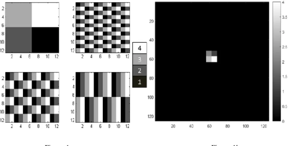
We generated five different image patterns which are modifications of those published by Sugama Chicklore et al. [35]. Their data were defined in a 10x10 matrix. We extended the matrix size to 12x12 to keep the periodicity of the image pixels, thus allowing further extension of the matrix dimensions (Fig. 1a). We also created a homogeneous constant matrix (A0) with the same matrix size. Then we arbitrarily inserted the matrices into a 128*128 image (Fig. 1b), and finally each
were converted to DICOM format using Matlab version 2014b (The MathWorks Inc., Natick, MA).
Figure 1a Figure 1b
The proposed A1, A2, A3 and A4 12x12 matrices (1a), and a representative final image that was created by inserting the A1 matrix into a black background (1b). The A1-A4 basic matrices contain
only four different pixel values (1-4) and the background area is set to zero in each final image.
2.2 Selected Heterogeneity Indices and the Fundamental Calculation Method
First, we calculated global (histogram-based) and local heterogeneity parameters of the A0, A1, A2, A3 and A4 matrices manually, without applying any software package (manual calculation). The global parameters were histogram-based values, which include the maximum (max), minimum (min), mean, standard deviation (SD), skewness, kurtosis and SD/mean parameters. Additionally, local parameters based on the co-occurrence matrix (coM) were also calculated:
contrast, correlation, energy, homogeneity, dissimilarity, and entropy.
Mathematical formulas of these parameters are provided in Table 1. Although other textural parameters can also be defined based on the GLCM, we investigated the most frequently used ones [5]. For the comparisons, manual calculation following these formulas was selected as the “gold standard”. The GLCM-based HI values were calculated with two different gray scale normalizations (8 and 64 levels), and 2 different directions (corresponding to 0o and 90o). Finally, each GLCM was normalized by dividing it by the sum of all matrix values.
Table 1
Formulas for the texture indices based on the co-occurrence matrix. Pij is the element in the ith row and jth column of the co-occurrence matrix. The μi, σi, and μj, σj parameters designate the weighted mean
and variance in row i and column j of the co-occurrence matrix, respectively. N is the size of the co- occurrence matrix.
Correlation
𝑃𝑖,𝑗∙ (𝑖 − 𝜇𝑖)(𝑗 − 𝜇𝑗) (𝜎𝑖2)(𝜎𝑗2)
𝑁−1
𝑖,𝑗 =0
where
𝜇𝑖= 𝑖 ∙ 𝑃𝑖,𝑗
𝑁−1
𝑖,𝑗 =0
and
𝜇𝑗= 𝑗 ∙ 𝑃𝑖,𝑗
𝑁−1
𝑖,𝑗 =0
𝜎𝑖2= 𝑃𝑖,𝑗∙ (𝑖 − 𝜇𝑖)2
𝑁−1
𝑖,𝑗 =0
𝜎𝑗2= 𝑃𝑖,𝑗∙ (𝑗 − 𝜇𝑗)2
𝑁−1
𝑖,𝑗 =0
Contrast
𝑃𝑖,𝑗∙ (𝑖 − 𝑗)2
𝑁−1
𝑖,𝑗 =0
Energy
𝑃𝑖,𝑗∙ |i − j|
𝑁−1
𝑖,𝑗 =0
Dissimilarity
𝑃𝑖,𝑗2
𝑁−1
𝑖,𝑗 =0
Homogeneity 𝑃
𝑖,𝑗
1 + |𝑖 − 𝑗|
𝑁−1
𝑖,𝑗 =0
Entropy
or
𝑃𝑖,𝑗∙ (− 𝑙𝑜𝑔2𝑃𝑖,𝑗)
𝑁−1
𝑖,𝑗 =0
𝑃𝑖,𝑗∙ (− ln 𝑃𝑖,𝑗)
𝑁−1
𝑖,𝑗 =0
2.3 Heterogeneity Index Calculations using Different Software Tools
The heterogeneity parameters of the DICOM images were computed with CGITA, InterView Fusion (ver. 2.02.055), Matlab and MaZda. Of the programs mentioned in the introduction, only these four were available at our institution at the time of our study. The parameters were then compared to the manually calculated values.
The 12x12 regions were segmented from the images based on both the vendor- supplied manual ROI definition method, and a semi-automatic segmentation method using a low threshold value; the resulting volumes were found exactly the same.
Based on the available software documentation, we found four different implementations of GLCM generation. CGITA computes local heterogeneity parameters by averaging the two GLCMs from horizontal and vertical (0o and 90o) directions [10]. In contrast, InterView Fusion calculates 26 different GLCMs (related to 26 different directions), then the average of these serves as the base for any HI. Matlab has built-in functions such as graycomatrix() and graycoprops();
the direction and the distance can be specified by the user [15]. We used the same directions as in the manual calculations. In MaZda, 20 different options are implemented in the following vector forms: [d 0], [0 d], [d d], [d –d], where d (distance) can take values of 1, 2, 3, 4, or 5.
2.4 Images for Analyzing the Reliability of Heterogeneity Parameters
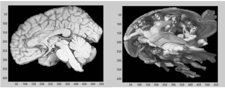
For these tests 2 images were selected: a sagittal histological section of the brain (Fig. 2a) [36], and Michelangelo's famous painting [37], the Creation of Adam (Fig. 2b). While the appearance and shape of these images is remarkably similar, as revealed by Suk et al. [38], the actual pattern and texture is different. For proper comparison we resampled the original photos to the same pixel size (418x559) and extracted the area of the brain shape from both images by removing the outside pixels using the method described by Zhenjiang et al. [39]; all heterogeneity parameters were calculated within the pixels inside. In this reliability analysis several other TIs were included using a Matlab-based software tool (referred by GLCM_feature) developed by A. Uppuluri [40].
This tool comprises the following 22 TIs: autocorrelation (autoc), contrast (contr), correlation_m (corrm), correlation_p (corrp), cluster prominence (cprom), cluster shade (cshad), dissimilarity (dissi), energy (energy), entropy (entro), homogeneity_m (homom), homogeneity_p (homop), maximum probability (maxpr), sum of squares (sosvh), sum average (savgh), sum variance (svarh), sum entropy (senth), difference variance (dvarh), difference entropy (denth), information measure of correlation1 (inf1h), information measure of correlation2 (inf2h), inverse difference normalized (indnc), and inverse difference moment normalized (indmnc). The detailed definitions of the above parameters can be found in the articles of [41, 42]. We also investigated how the parameters depend on the number of gray scale normalization (with 8, 16, 32, 64, …, 1024 levels) in the case of 6 selected TIs (contrast, correlation, energy, homogeneity, dissimilarity, and entropy).
Figure 2a Figure 2b
Segmented histological section of the brain (2a), and Michelangelo's segmented famous painting, the
“Creation of Adam” (2b). The pixel size and the colormap are the same for both cases (418x559 and gray scale).
3 Results
3.1 Texture Index Values using Different Software
The ratio of high and low signal intensities and the global data (as listed in section 2.2) were equal in all four inhomogeneous images. The images were structured so that the values of the local parameters, when calculated in the horizontal direction for images A2, A3 and A4, remain the same. The values of the global parameters such as max, min, mean, SD, skewness, kurtosis and SD/mean (Tables 2) for matrices A1-A4 were very similar. With Matlab and CGITA the kurtosis values were significantly different from the manually calculated ones. For the rest of the global parameters the discrepancy was below 0.5% in all cases. From here on all results are given as the percentage differences between the output of the respective software and manual calculation. Differences were even more pronounced in the case of co-occurrence matrix based local parameters (contrast, correlation, energy, homogeneity, dissimilarity and entropy) for both 8 and 64 level gray scale normalization. When we used Matlab and MaZda, calculations were carried out in both [0 1] and [1 0] directions. After 8 level gray scale normalization (Fig. 3), the largest percentage discrepancy was seen for HI values provided by MaZda (both directions), and CGITA.
Table 2
Global HI results for matrices A0 (left), and A1-A4 (right). Some parameters are not available (n.a.) for homogeneous images (Man. = manual calculation).
For matrix A1 the contrast values showed 75-82% deviations with MaZda (both directions), and ~47% with CGITA. When correlation HI was calculated from matrices A2, A3, and A4, we also saw a significant difference between software- aided and manual calculations. The energy parameter yielded a difference of
~50% with MaZda ([1 0] direction) and nearly 70% with CGITA.
Figure 3
Percentage differences between the values of local parameters (y-axis), provided by the four different software packages, and manual calculation (after 8 level gray scale normalization). Panels A, B, C and
D show the results for the four different synthetic images.
Parameters Matlab MaZda IW- Fusion
CGITA Man. Matlab MaZda IW- Fusion
CGITA Man.
A0 A1, A2, A3, A4
Mean 100 100 100 100 100 2.500 2.500 2.500 2.500 2.500
Min 100 100 100 100 100 1.000 1.000 1.000 1.000 1.000
Max 100 100 100 100 100 4.000 4.000 4.000 4.000 4.000
SD n.a. 1.122 1.118 1.120 1.118 1.120
Skewness 0.000 0.000 n.a. 0.000 0.000
Kurtosis 1.640 -1.360 -1.360 1.640 -1.360
SD/Mean 0.449 n.a. n.a. 0.447 0.448
Homogeneity and dissimilarity could not be calculated with MaZda. In the case of Matlab (regarding both directions) all HI parameters had a percentage difference from manual calculation less than 0.5%. The eight level, gray scale normalization was not available with InterView Fusion. Homogeneity and entropy showed 5- 45% and 10-20% biases, respectively, for all matrices when the 64 level, gray scale normalization was carried out with InterView Fusion (Fig. 4). In case of CGITA, contrast and dissimilarity showed nearly 50% difference for matrix A1, dissimilarity showed a difference greater than 100% for matrix A2, and energy showed a nearly 60% difference for matrices A3 and A4. The largest percentage differences were seen in case of CGITA. Matlab calculations (in both directions) resulted in a maximum difference of 2%. Sixty-four level gray scale normalization was not available in MaZda, and nor contrast, correlation, energy or dissimilarity could be calculated with the built-in modules of InterView Fusion.
Figure 4
Percentage differences of the values of local parameters (y-axis), provided by the four different software packages from manual calculation (after 64 level gray scale normalization). Panels A, B, C
and D show the results for the four different synthetic images.
It can also be stated from Figs 3-4 and Table 2 that all global parameters obtained by the four different software packages were very similar to those calculated manually (<1% deviations), and the values for the four patterns were almost identical, as they must be due to their construction.
In case of local parameters, calculations done with Matlab yielded the smallest difference from the manual calculation. We obtained the most accurate local parameter values using Matlab. Furthermore, for matrices A2, A3, and A4, the local parameters in the horizontal direction gave the same results with Matlab,
Mazda and manual calculation, as expected based on the definition of the matrices [43].
For further analysis the absolute values of HIs were also compared for all software and calculation methods. Figs 5, 6 and 7 present each TIs with both normalizations and for all images (A1, A2, A3 and A4). The horizontal axis presents the different software and calculation methods. If a method allowed to generate coM matrix for 2 different directions ([0 1] and [1 0] (which was the case with Manual, Matlab and MaZda), the mean values were also calculated.
From these images we got the same TI values at horizontal direction [0 1] for A2, A3 and A4, corresponding to the definition of these images. Although we found large percentage differences between the software packages, similar monotony (in the order of A1…A4 images) can be seen from Fig. 5 and 6 in case of Manual mean, Matlab mean, MaZda mean, CGITA and InterView Fusion. Entropy and energy (Fig. 7) do not show a similar behavior. The formulas of energy and entropy depend on the Pij value of the co-occurrence matrix element rather than the row and column indices (i,j), thus gray level normalization had smaller effect on these TIs. This is demonstrated in Fig. 7; the indices from 8 and 64 level normalization are very similar. Fig. 8 presents the percentage difference (PD) of TIs between 8 and 64 gray level normalization for three calculation methods:
Manual mean, Matlab mean and CGITA.
Figure 5
Comparison of contrast and dissimilarity between all software and calculation methods, with both normalizations (8 and 64), and for all images (A1, A2, A3 and A4). The [0 1] and [1 0] symbols stand
for the horizontal and vertical directions, respectively.
Figure 6
Comparison of correlation and homogeneity between all software and calculation methods, with both normalizations, and for all images
Figure 7
Comparison of energy and entropy between all software and calculation methods, with both normalizations, and for all images
Figure 8
Percentage difference of selected TIs between the 8 and 64 gray level normalization in case of all images, for three calculation methods: Manual mean, Matlab mean and CGITA
Figure 9
Dependence of contrast and dissimilarity on the normalization level (8 to 512), calculated from the A3 matrix in 3 directions ([0 1], [1 0], [-1 1]. The axes of the contrast plot are scaled in log-log format, allowing for better visualization of the power relationship between the contrast and the normalization
level.
MaZda and InterView Fusion are missing from this comparison, because they use a fixed number of gray levels (8 or 64). In Fig. 8 contrast and dissimilarity show very similar tendencies which is due to the similarity of their formulas (Table 1), including the same factor (i-j) in the numerator. It can also be noted that the PDs of contrast and dissimilarity are exactly the same for the three calculation methods. The tendency of homogeneity is reversed, since its formula contains the factor (i-j) in the denominator. The values of energy and entropy do not depend on the normalization level, as shown in Fig. 7.
We also analyzed the gray level dependences more details in the case of the contrast and the dissimilarity. Fig. 9 shows the TIs from the A3 matrix while the normalization level changed from 8 to 512. The trend is linear and quadratic for dissimilarity and contrast, respectively, corresponding to the power of the (i-j) factor in their formulas.
3.2 Results of Reliability Analysis of the Heterogeneity Parameters
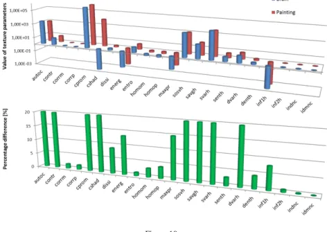
Fig. 10 shows the 22 texture index values calculated by the GLCM_feature tool (upper panel) for the histological slice of the brain, and Michelangelo's painting.
Figure 10
Values of the 22 texture parameters for the histological section of the brain and Michelangelo's painting, and the related percentage differences of the TIs. In the latter case, the scale of the vertical
axis is set arbitrarily to 20%, allowing better visualization of the smaller values.
The lower panel presents the percentage differences of the related TIs between the two images. Interestingly, from the 22 co-occurrence based texture parameters, 12 indices did not show relevant differences (less than 10%: corm, corrp, entropy, homom, homop, senth, denth, inf2h, indnc, idmnc, dissi and inf1h). In addition, 5 indices depicted differences in the range of 10-20% (contr, cprom, energy, maxpr, dvarh), and only 5 parameters presented more than 20% dissimilarities (autoc, cshad, sosvh, savgh, svarh). Selecting the contrast, correlation, energy, homogeneity, dissimilarity, and entropy parameters, we also calculated the percentage differences between the two images at distinct gray levels (Fig. 11).
This graph confirms that the TI differences did not change when the gray level number was more than 64. In other words, at least 64 normalization levels need to be used for reliable, stable results. These findings suggest that images with similar overall appearance but with different content may have texture indices with very similar values.
Figure 11
Percentage differences of contrast, correlation, energy, homogeneity, dissimilarity and entropy between the two images, using different numbers of gray levels (from 8 to 1024)
4 Discussion
Texture analysis studies provide additional quantitative information about medical images, which may help with the characterization and differentiation of healthy and pathological areas, and with grading [44, 45, 46, 47]. Several free and commercial software tools such as Matlab, MaZda, InterView Fusion, CGITA, TexRad and ImageJ implement the calculation of heterogeneity parameters;
however, in many cases, the implemented calculation algorithms are unknown [8, 10, 15, 29, 48, 49].
In our work, we studied the texture calculation mechanisms of four biomedical software packages; we compared the heterogeneity parameters provided by Matlab, MaZda, CGITA, and InterView Fusion to those calculated manually.
Our aim was to compare various heterogeneity indices, and to highlight possible reasons for the differences. We used 4+1 synthetic images, and we calculated local and global heterogeneity indices after both 8 and 64 level gray scale normalization. Global parameters (histogram-based calculations, Table 2) by all four programs were very similar to the values calculated manually (<0.5%) in case of all five matrices (A0-A4).
We found more differences among the results of local parameters (Figs 3-4). The smallest percentage difference was seen between Matlab and manual calculations for both gray scale normalization settings, in both [0 1] and [1 0] directions. For matrices A2, A3, and A4, Matlab, MaZda and manual calculation yielded similar local parameter values, when choosing horizontal direction of calculation. An explanation for the HI differences may be that the (undocumented) way of averaging when forming multidirectional co-occurrence matrices may also differ.
The formulas used for the manual calculations may also differ from those implemented in the software packages tested, although their names may be the same.
For instance, in CGITA, based on the program code, it is clear that the horizontal and vertical calculations are done in a single step, thus a certain averaging takes place [46]. CGITA does not use the built-in Matlab functions for the co- occurrence matrix calculations. InterView Fusion is not an open-source software;
thus the particular algorithms are unknown, but based on personal communication we suspect that the co-occurrence matrix calculations are done in 3 dimensions.
Not both levels of normalization (8 and 64) are available in all the packages, nor is the definition of the [0 1], [1 0] directions the same, thus the values of heterogeneity parameters provided by the different programs are not comparable.
In addition, we analyzed how the selected HIs depend on normalization levels.
Our results indicate that contrast and dissimilarity behave alike, because they both include the same factor (i-j) in the numerator (Fig. 5). On the other hand, energy and entropy do not depend on the normalization level. In general, similar monotony (in the order of A1…A4 images) of the texture indices can be seen in
Fig. 5-7, independently of the software or methods applied. In the next step we focused on the reliability of HIs based on two selected images (Fig. 2), a famous painting and a histological brain slice. These two segmented images have the same pixel size and very similar shape, but the actual patterns and textures are quite different. From the calculated 22 TIs, only 5 parameters depict more than 20%
dissimilarities, even though we used two images with different texture properties (Fig. 10). Based on our analysis, at least 64 normalization levels need to be used for reliable results (Fig. 11).
Conclusion
CGITA, InterView Fusion, Matlab and MaZda calculate the co-occurrence based heterogeneity indices differently, thus, the results of these calculations are not comparable. Our comparison also underlines that, in medical multi-center studies it is especially critical to use the same software package for all patients.
Furthermore, it would be necessary to accept and implement a standard algorithm in such software, so that the results would be truly comparable among different programs. Standardized texture analysis algorithms would then better aid medical diagnostics, therapy planning, follow-up studies and they might provide a non- invasive classification of pathological lesions as well.
Our study also confirmed that some TIs can be very similar in spite of the images having different texture. It means that a single parameter cannot properly characterize a segmented area and using a group of several textural parameters may be more accurate. Some texture parameters are not reliable when distinguishing different changes in patterns, so texture analysis should be clinically validated and used with caution.
Acknowledgements
This work was supported by the „Richter Gedeon Talentum Alapítvány”.
References
[1] Yip SS, Aerts HJ (2016) Applications and limitations of radiomics, Phys.
Med. Biol. 61:150-166
[2] Lerski RA, Straughan K, Schad LR, Boyce D, Blüml S, Zuna I (1993) MR image texture analysis - an approach to tissue characterization. Magn.
Reson. Imaging. 11: 873-887
[3] Ahmadvand A, Daliri MR (2016) Invariant texture classification using a spatial filter bank in multi-resolution analysis. Image Vis Comput 45:1-10 [4] Maani R, Kalra S, Yang Y-H (2013) Noise robust rotation invariant
features for texture classification. Pattern Recognit 46:2103-2116
[5] Haralick RM, Shanmugam K, Dinstein I (1973) Textural features for image classification. IEEE Trans Syst Man Cybern 3:610-621
[6] Brooks FJ (2013) On some misconceptions about tumor heterogeneity quantification. Eur J Nucl Med Mol Imaging 46: 1292-1294
[7] Strzelecki M, Szczypinski P, Materka A, Klepaczko A (2013) A software tool for automatic classification and segmentation of 2D/3D medical images. Nucl Instruments Methods Phys Res Sect A Accel Spectrometers, Detect Assoc Equip. doi: 10.1016/j.nima.2012.09.006
[8] Szczypinski PM, Strzelecki M, Materka A, Klepaczko A (2009) MaZda - a software package for image texture analysis. Comput Methods Programs Biomed 94:66-76
[9] Szczypinski PM, Strzelecki M, Materka A (2007) Mazda - a software for texture analysis. In: 2007 International Symposium on Information Technology Convergence (ISITC 2007). IEEE, pp. 245-249
[10] Fang Y-HD, Lin C-Y, Shih M-J, et al (2014) Development and evaluation of an open-source software package „CGITA” for quantifying tumor heterogeneity with molecular images. Biomed Res Int 2014:248505 [11] Available from:
https://github.com/cmci/GLCM2/blob/master/src/main/java/emblcmci/glcm /GLCM_TextureToo.java [accessed 2018. 03. 20]
[12] Available from:
https://imagej.nih.gov/ij/plugins/download/GLCM_Texture.java [accessed 2018. 03. 20]
[13] Baecker V (2010) Workshop: Image processing and analysis with ImageJ and MRI Cell Image Analyzer. Image (Rochester, NY) 1-93
[14] Abramoff MD, Magalhães PJ, Ram SJ (2004) Image processing with ImageJ. Biophotonics Int. 11:36-42
[15] Available from: http://www.mathworks.com/help/images/texture-analysis- 1.html [accessed 2017. 03. 20]
[16] Pantic I, Nesic Z, Paunovic Pantic J, et al (2016) Fractal analysis and Gray level co-occurrence matrix method for evaluation of reperfusion injury in kidney medulla. J Theor Biol 397:61-7
[17] J. E. Cabrera: Texture Analyzer
https://imagej.nih.gov/ij/plugins/texture.html [accessed 2017. 03. 20]
[18] Wang XC, Mo JL, Ouyang H, et al (2015) Squeal noise of friction material with groove textured surface: an experimental and numerical analysis. J Tribol 138:021401
[19] Bastos FS, Oliveira EA, Fonseca LG, et al (2016) A FEM-based study on the influence of skewness and kurtosis surface texture parameters in human dental occlusal contact. J Comput Appl Math 295:139-148
[20] Yan D, de Beurs KM (2016) Mapping the distributions of C3 and C4 grasses in the mixedgrass prairies of southwest Oklahoma using the Random Forest classification algorithm. Int J Appl Earth Obs Geoinf 47:125-138
[21] de Albuquerque M, Anjos LG V, Maia Tavares de Andrade H, et al (2016) MRI texture analysis reveals deep gray nuclei damage in amyotrophic lateral sclerosis. J Neuroimaging 26:201-6
[22] Yan L, Liu Z, Wang G, et al (2015) Angiomyolipoma with minimal fat:
differentiation from clear cell renal cell carcinoma and papillary renal cell carcinoma by texture analysis on CT images. Acad Radiol 22:1115-21 [23] Orphanidou-Vlachou E, Vlachos N, Davies NP, et al (2014) Texture
analysis of T1 - and T2 - weighted MR images and use of probabilistic neural network to discriminate posterior fossa tumours in children. NMR Biomed 27:632-9
[24] MacKay JW, Murray PJ, Kasmai B, et al (2016) MRI texture analysis of subchondral bone at the tibial plateau. Eur Radiol 26:3034-3045
[25] Daginawala N, Li B, Buch K, et al (2016) Using texture analyses of contrast enhanced CT to assess hepatic fibrosis. Eur J Radiol 85:511-517 [26] Liu W, Raben N, Ralston E (2013) Quantitative evaluation of skeletal
muscle defects in second harmonic generation images. J Biomed Opt 18:26005. doi: 10.1117/1.JBO.18.2.026005
[27] Michoux N, Guillet A, Rommel D, et al (2015) Texture analysis of T2- weighted MR images to assess acute inflammation in brain MS lesions.
PLoS One 10:e0145497. doi:10.1371/journal.pone.0145497
[28] Wang H-M, Cheng N-M, Lee L-Y, et al (2016) Heterogeneity of 18 F-FDG PET combined with expression of EGFR may improve the prognostic stratification of advanced oropharyngeal carcinoma. Int J Cancer 138:731–
738
[29] Available from:
http://www.mediso.hu/products.php?fid=1,10,6&pid=67&feature=all [accessed 2018. 03. 20]
[30] Tixier F, Hatt M, Valla C, et al (2014) Visual versus quantitative assessment of intratumor 18FFDG PET uptake heterogeneity: prognostic value in non-small cell lung cancer. J Nucl Med55:1235-41
[31] Orlhac F, Soussan M, Chouahnia K, et al (2015) 18F-FDG PET-derived textural indices reflect tissue-specific uptake pattern in non-small cell lung cancer. PLoS One 10:e0145063 . doi: 10.1371/journal.pone.0145063 [32] Ganeshan B, Abaleke S, Young RCD, et al (2010) Texture analysis of non-
small cell lung cancer on unenhanced computed tomography: initial
evidence for a relationship with tumour glucose metabolism and stage.
Cancer Imaging 10:137-43
[33] Hayano K, Kulkarni NM, Duda DG, et al (2016) Exploration of imaging biomarkers for predicting survival of patients with advanced non–small cell lung cancer treated with antiangiogenic chemotherapy. Am J Roentgenol 206:987-993 . doi: 10.2214/AJR.15.15528
[34] Ahn SY, Park CM, Park SJ, et al (2015) Prognostic value of computed tomography texture features in non–small cell lung cancers treated with definitive concomitant chemoradiotherapy. Invest Radiol 50:719-725 [35] Chicklore S, Goh V, Siddique M, et al (2013) Quantifying tumour
heterogeneity in 18F-FDG PET/CT imaging by texture analysis. Eur J Nucl Med Mol Imaging 40:133-140
[36] Available from:
https://library.med.utah.edu/WebPath/HISTHTML/NEURANAT/CNS016 A.html [accessed 2018. 03. 20]
[37] Available from:
https://en.wikipedia.org/wiki/The_Creation_of_Adam#/media/File:Creaci
%C3%B3n_de_Ad%C3%A1n_(Miguel_%C3%81ngel).jpg, [accessed 2018. 03. 20]
[38] Suk I, Tamargo RJ (2010) Concealed neuroanatomy in Michelangelo's separation of light from darkness in the Sistine chapel. Neurosurg. 66: 851- 861
[39] Zhenjiang L, Yu M, Hongsheng L, Gang Y, Honglin W, Baosheng L (2016) Differentiating brain metastases from different pathological types of lung cancers using texture analysis of T1 postcontrast MR. Magn. Reson.
Med. 761410-1419 [40] Available from:
https://www.mathworks.com/matlabcentral/fileexchange/22354 [accessed 2018. 03. 20]
[41] Soh L, Tsatsoulis C (1999) Texture Analysis of SAR Sea Ice imagery using gray level cooccurrence matrices. EEE Trans. Geosci. Remote Sens. 372 [42] Available from:
http://murphylab.web.cmu.edu/publications/boland/boland_node26.html [accessed 2018. 03. 20]
[43] Castellano G, Bonilha L, Li LM, Cendes F (2004) Texture analysis of medical images. Clin Radiol 59:1061-1069
[44] Peikari M, Gangeh MJ, Zubovits J, et al (2016) Triaging diagnostically relevant regions from pathology whole slides of breast cancer: a texture based approach. IEEE Trans Med Imaging 35:307-315
[45] Rodriguez M, Rehn SM, Nyman RS, et al (1999) CT in malignancy grading and prognostic prediction of non-Hodgkin’s lymphoma. Acta Radiol 40:191-7
[46] Henry W (2010) Texture analysis methods for medical image
characterisation. Biomedical Imaging. InTech.
https://cdn.intechopen.com/pdfs-wm/10175.pdf [accessed 2018.03. 20]
[47] Available from: https://www.ucl.ac.uk/nuclear- medicine/research/researchabstracts/texrad [accessed 2018. 03. 20]
[48] Available from: http://texrad.com/papers-presentations/ [accessed 2018. 03.
20]
[49] Available from: https://code.google.com/archive/p/cgita/ [accessed 2018.
03. 20]