IDENTIFICATION IN TETE PRESENCE OF DRIFTBÁNYÁSZ Csilla

Magyar Tudományos Akadémia Számítástechnikai és Automatizálási Kutató Intézete Com puter and Automation Institute, Hungarian Academy o f Sciences

Institut für Rechentechnik und Automatisierung der Ungarischen Akademie der Wissenschaften Исследовательский Институт Вычислительной Техники и Автоматизации Венгерской Академии Н аук

* Н 1502 Budapest, XI. Kende utca 13-17, * Hungary * Ungarn * Венгрия *

IDENTIFICATION IN TETE PRESENCE OF DRIFT

BÁNYÁSZ Csilla

1972

A kiadásért felelős Dr. Vámos Tibor

az

MTA Számítástechnikai és Automatizálási Kutató Intézetének

igazgatója

Készült az Országos Műszaki Könyvtár és Dokumentációs Központ házi sokszorosítójában

F.v.:Janoch Gyula

Professzor K.J.8 ström meghívására 1 9 7 2 .májusától 3 hónapos tanulmányúton vettem részt a Lundi Műszaki Egyetem Automatizálási Tanszékén /Lund Institute of Technology, Division of Automatic Control/.

Jelen összefoglaló az ott végzett munka egy részét tartalmazza.

3

TA B L E OF CONTENTS

Page

1. Introduction ... 7

2. Measuring errors in the output signal in one or several points ... 11

3. Constant level on the output ... 17

4. Linear d r i f t ... 36

5. Sinusoidal drift ... 42

6 . Summary and conclusions ... 47

7. References ... 48

8 . Acknowledgements ... 49

4

ABSTRACT

In this report the influence of drift of different types and m a g ­ nitude on the ML and LS identification is examined. The drift effects are simulated, after identifying the results are analysed. It can be seen from the results that the presence of drift depending on the magnitude and type of it can have a significant influence on the parameter estimates. This means that it is neccessary to analyse the measurements before the

identification, in many cases more exact demands have to be created on the measuring conditions or prefiltering strategies must be applied.

5

1. INTRODUCTION

During the identification from industrial data the problem appears usually whether the measurements correspond to the real values of signals or not, fulfil the requirements of the identification methods otherwise what the influence of inadequate data is for the estimation.

Starting from these ideas the problem was approached in the follow­

ing way: the input signals were PRBS and the output signals of the process were computed by simulation /supposing correlated noise at the output/. Then different types of modifications were performed on the output data and after the identification from the input - and the modified values of output it was possible to draw some conclusions about the influence of drift of different character and magnitude on the identification.

We use the term drift in a very extended meaning, i.e. the following cases were considered:

1/ The values of output were changed in one or several points 2/ A constant level was added to the values of output

3/ A level changing linearly was added to the values of output 4/ A sinusoidal signal was added to the output.

I

The cases 1/ and 2/ are used as typical situations for industrial measurements and our aim is to examine the influence of the erroneous measurements on the estimates i.e. we do not filter the data before the identification.

The third case Is generally considered as a typical drift effect.

The fourth situation can appear in practice in the case of superposed signals.

In this paper we restrict ourselves to the examination of influence of drift in the output since we have used the off-line m a x i m u m likelihood method /ML/ [l] for the identification and the input signal PRBS was given to the process b y us. In the first step this method produces the least- -squares /LS/ estimates of process paramters so we can compare them with .the ML ones for the different types of the drift effects. /I used the ML

7

identification p r o g r a m in the program library of UNIVAC 1108 made by I.Gustavsson М / .

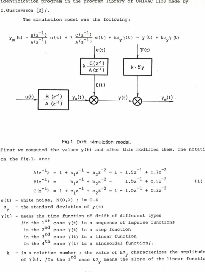
The simulation model was the following:

^ m (t) B(z u(t) + X C-\ z e (t) + ko y(t ) = y(t) + ko V (t)

A(z_ 1 ) A(z 1 ) y y

Fig. 1. Drift simulation model.

F i r s t we computed the values y(t) and after this modified them. The notations on the Fig.l. are:

- 1, В (z 1) = C (:-Is

: 1 + a^z 1 + a 2z-2 = 1 - 1 .5z~ 1 + О N b ^ 1 + b 2z" 2 = l.Oz-1 + 0 .5z : 1 + C^z 1 + c 2z“ 2 = 1 - l.Oz" 1 + 0 .2z

N (О, Л ) ; X-= 0.4

- 2 - 2 - 2

(1 )

a — the standard deviation of y(t)

V

Y (t 1 - means the time function of drift of different types fin the 1st case y(t) is a sequence of impulse functions

n J

in the 2r case Y(t) is a step function in the 3 case Y (t) is a linear function

in the 4th case Y(t) is a sinusoidal function/.

к — is a relative number ; the value of ko^. characterizes the amplitude of Y (t) . /In the 3rd case kcy means the slope of the linear function./

The number of samples was N = 500.

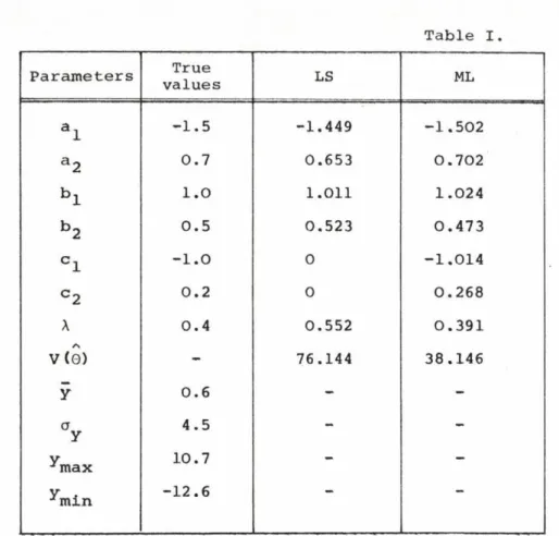
The results obtained b y identification for the case without drift can

8

be seen in Table I. and the time functions of the input, output, mode output, model error, residual are shown on Fig.2.

4

‘ on Toon мора е д о щи wopö î7® ô нооо

Table I Parameters True

values LS ML

a l -1.5 -1.449 -1.502

a 2 0.7 0.653 0.702

b l 1.0 1.011 1.024

cr

c i - 1.0 0 -1.014

c 2 0.2 0 0.268

A

Л

V ( 0 ) 76.144 38.146

ÿ

a

У 4.5 - -

уJ m a x 10.7 -

^ m i n -12.6

'

Estimations from the data without drift. N=500

lo

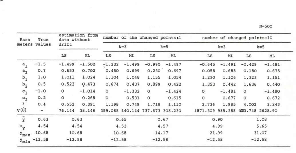
2. M E A S U R I N G ERRORS IN THE O U T P U T SIGNAL IN ONE OR SEVERAL POINTS

During the simulation of this situtation we changed one or more output values in the following way:

y (t) = y (t) + ko Y(t)

m y

where now T (t) is an impulse function series, i.e.

(2)

1 if t = 25,75,125,...,475. /or t - 2 5 0 / T (t) =

О otherwise

Fig.3.

The identification was performed from the input and the modified output values. The ML estimates obtained in this way are shown in the Table

II. together with the least-squares estimates. It can be seen from Table II.

that the estimates of a^, b^ are reasonable good but the estimates of c.^ are increasingly worse if the к is increasing and the values of 6 ^ tend to the values of the corresponding when the number of the changed points is 1 and 10, as well. The reason for this can be seen easily because in this case the noise by the side of the signal kay y(t) appearing in discrete time points

/or only in one point/ at the output is negligible and this situation can be identified only by such an identification model in which C(z = A(z .

11

K)

N=500 Para

meters

True values

estimation from data without drift

LS ML

number of the changed points:! number of changed points:10

k==3 k==5 k=3 k= 5

LS ML LS ML LS ML LS ML

a l -1.5 -1.499 -1.502 -1.232 -1.499 -0.990 -1.497 -0.645 -1.491 -0.429 -1.481

»2 0.7 0.653 0.702 0.450 0.699 0.230 0.697 0.058 0.688 0.180 0.675

b l 1.0 1.011 1.024 1.104 1.048 1.155 1.054 1.230 1.106 1.323 1.151

b 2 0.5 0.523 Ç.473 0.674 0.437 0.899 0.422 1.353 0.442 1.636 0.440

C 1 - 1.0 0 -1.014 0 -1.332 0 -1.424 0 -1.481 0 -1.480

c 2 0.2 0 0.268 0 0.531 0 0.615 0 0.677 0 0.672

Л 0.4 0.552 0.391 1.198 0.749 1.718 1.110 2.736 1.985 4.002 3.243

V (o) - 76.144 38.146 359.068 140.144 737.673 308.230 1871.309 985.388 4003.748 2628.90

Ÿ ^{0.63 0 .63 0.65 0.67 0.90 1 .08}

a y 4.54 4. 54 4.53 4.57 4.99 5. 65

V2max 10.68 1 0 .68 10.68 14.17 21.99 31. 07

^min -12.58 - 1 2 .58 -12.58 -12.58 -12.58 -1 2 .58

Table I I . Estimates in the case of measuring errors

кбу Т( t )

u(t) В (z-1 ) y0 ( O x

X

A(z-i ) v y - —

Fig. A.

It can also be seen from Table II. that these statements are not valid for the least-squares estimation because resulting from the behaviour of LS method it tries to smooth over the high jumpings in the output so the LS estimates of a^ and b^ are also spoiled.

These establishments can also be observed on the time functions on Fig.5. and Fig.6 . both for the ML and LS estimations.

13

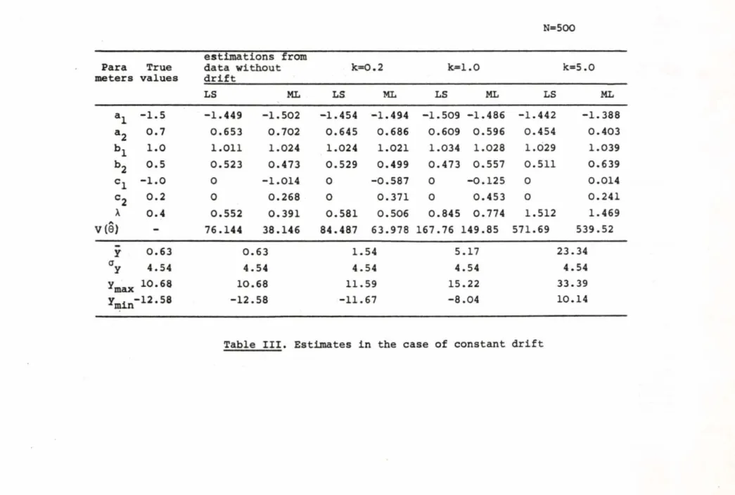
N=500

Para meters

True values

estimations from data without drift

k= 0 .2 k=l .0 k = 5 .0

LS ML LS ML LS ML LS ML

al -1.5 -1.449 -1.502 -1.454 -1.494 -1.509 -1.486 -1.442 -1.388

a 2 0.7 0.653 0.702 0.645 0.686 0.609 0.596 0.454 0.403

bx 1.0 1.011 1.024 1.024 1.021 1.034 1.028 1.029 1.039

b 2 0.5 0.523 0.473 0.529 0.499 0.473 0.557 0.511 0.639

C 1 - 1.0 0 -1.014 0 -0.587 0 -0.125 0 0.014

= 2 0.2 0 0.268 0 0.371 0 0.453 0 0.241

X 0.4 0.552 0.391 0.581 0.506 0.845 0.774 1.512 1.469

V (0) - 76.144 38.146 84.487 63.978 167.76 149.85 !571.69 539.52

Ÿ 0.63 0 .63 1 .54 5.17 23.34

a

У 4.54 4. 54 4. 54 4.54 <1.54

ул max 10.68 1 0 .68 1 1 .59 15.22 33.39

w 1 2 -58 - 1 2 .58 -1 1 .67 -8.04 10.14

Table III. Estimates in the case of constant drift

3. C O N S T A N T LEVEL ON THE OUTPUT

The simulated output is generated by the following equation:

Ym (t) = y(t) + kcJyY (t) (3) where now Y (t) is a unit step signal.

The identified values of parameters can be seen in Table III. for different values of k. It is striking that the increasing value of к has the biggest influence for a^ and c^. Analysing the results we can establish that the values of a^,a2 are formed in such way that the sum l+a1+a2 tends to 0, the values of c^ and the rootte of the polynomial c(z *) are in Fig.8 . for different values of к where the roots seem to be moving to a certain point.

In order to interpret this effect we have examined some different cases.

17

A

Fig.8.

18

3.1

First let us consider a simple case when the process model is :

ym(t)

CU-1)

ym (t) = tlz t(t) where it is assumed that e(t) is white noise.

Then

( 4 )

(5)

Let us write the loss function for a first order systemt

The necessary condition for the extremum is :

Exact analytical solution can not be given because of the complexity of this equation. Two special cases are examined, k=0 and к-*-” .

In the case of k=0 we have

L9

We get the e q u a t i o n

if H +i

cc! + c(l + c 2 )- c = О (1 0)

Solutions of (10) are c=c , c=^ where the first one is admissible for the stable system in case without drift.

In the case of кг*-" the equality 2o 2

---- £--- = О (11)

( 1 + Ô ) 3

must be fulfilled and this is possible only in the case when Ô-*-® but under the restrictions of stability c=l. /During the identification the ML method allows only stable polynomial C(z Ъ .)

The solution ô=l can also be obtained from (8) because if yg = О is fulfilled then we can write that:

For k-*-00 this can be true only when c = l .

3.2

Now let us consider a second order system for this simple model. Then the loss function is:

E q u ating the derivatives to zero we get the following equations:

These are complicated functions of c^ and c 2 and can not be handled analytically.

Examining the case k -*00 the equality 2 a

(l+c1+c2)

= О (16)

must be lulfilled /this is valid both for (14) and (15)/ which is true only if c^ and c ^ 00 . But under the stability conditions the admissible domain for c^,c2 can be seen on Fig.9. /striped domain/ so only the values c^=2 , 62=1 are attainable as a maximum. On the other hand this solution makes it possible to fulfil the conditions = О and = О in the case of k'*", i.e. the first term of (14) and (15) is made infinite.

21

This solution concerning the roots of the polynomial ê(z means a double root on the z-plane in the point -1 .

A

Fig. 9-

The parameter values obtained by the simulation and identification of model (4) can be seen in Table III./a for second order system. The changing of and and the roots of C (z are also presented for different к on F i g . 10. and this figure is similar to Fig.8 /a.,8 /b.

But on the basis of previous examinations we can not conclude that these statements are also valid for the general case because the model (4) does not include the parameters a^.

22

o>

Table I I I . /а

Para­

meters

True values

ML

k=l k=5

a l 0 - -

a 2 О - -

b l 0 - -

b 2 0 - -

C 1 - 1.0 -0.218 0.657

C 2 0.2 0.513 0.622

A

A

V(0) — 124.786 619.113

ÿ

Oy 0.563 0.563 0.563

y __ _{2.23 4.47}

Jmax

^min — -1.25 0,98

N=500

Л

S’2

1

\

TRUE x

1 k = 5 / ~

X

- 1 1

- 1

л C<

Fig 10.

23

3.3

Let us consider the following model:

ym (t) = e(t)

+ kV (t>

which is identified b y the model:

Ô (z Ь

ym( t ) = _{A (z} -ТГ₎ ^e(t) Then

E (t) = К ( z 1 ) C ( z ^ ) C (z-1 ) A ( z -1)

e ( t ) + ко Y(t) C(z Ъ Y

(17)

(18)

(19)

and assuming that e (t) is white noise the loss function for a first order system is :

F = E U 2 ( t )} 1 2"j

(l+az ^)(l+cz ( l+az)(1+cz) dz (l+az *) ( 1+cz *) ( l+az)( 1+cz) z k 2a 2 (l+a)2

+ — * --- 5—

(1+ с Г

(l+â'1+2âc+c2+ â 2c 2)( l+â2ç 2 ) -2 (a+c) ( â+c)( 1+âc ) + 2âc( a 2+ 2ac+c2-ac-a2ç 2) (1-ac)(l+a2c 2-a2-c2 )

(1+ â )2 (1+ 8 ) 2

2 2

k ^ (2 0)

Rewriting the equation ( 20) so that the numerator of the first term is marked by N, the denominator by D, i.e.

F N + (l+a)2 D (1+c)2

2 2

к u ₍₂₁₎

we can write the necessary conditions for the derivatives:

3F N â D - N Dl 2 (l+a) 2 2

<*a

D (l+S)

T

24

NX D

C (22a)

3F

л A

9c

- N D(

c 2 (1+ â )2

(1+ Ô )3 * 4 ^О

where NX and DX mean the derivatives with respect to â of numerator and

3 â

denominator, Ng , Dg the derivatives of N and D with respect to 6 . These equations are so complicated functions of â and 6 that they can not be handled analytically.

Let us take the case k -*00 . Now there are two possibilities for sat­

isfying equations ( 22), ( 22a) for k-*-®. One of them is that â = - l , the other one is that 0 = 1 ; this latter is equal to the previous one obtained for first order system taking account only stable solutions.

Examining the two terms of equations (22), (22a) the following equalities must be fulfilled:

and

N DX

a 2 ( 1+â )

(1+â)2

.

k ay

NX D

c - N DÁ

c 2 (1+ â )2 , 2 2 --- T~ k av (1+6) 3 Y from which we get that D must be О if k»-® .

Writing D in detail:

(23)

(24)

(l-a6 )(l+a2â 2-a2-â2 ) = 0 (25)

After rearranging we get:

(1-aô)(1-a2)( 1-c2) = 0 (26)

The solution 0=-l must be excluded because this value would make the right sides of equations (23), (24) infinite even in the case of a small k. From the solutions 6 = 1 , c=- the solution c=l is admissible taking account only

â

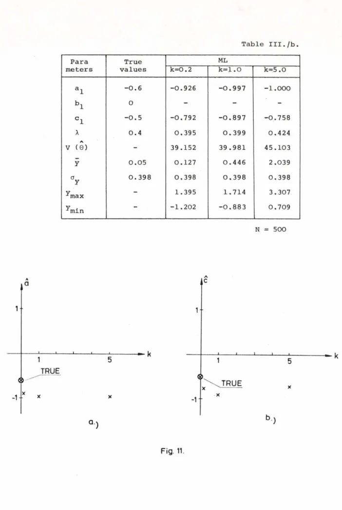
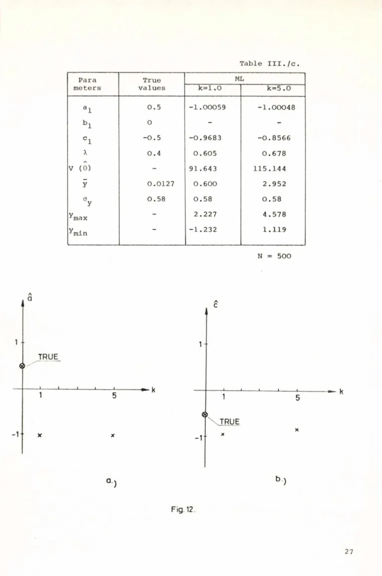
stable solutions and this is justified by simulation, too. See Table III./b, Table III . /с. and Figs. 11.,12. At the same time this value minimizes the right side terms of equations ( 23), (24 ).

Table I I I . /Ь

Рага True ML

meters values k = 0 .2 *■ II i-1 О II U1 О

a l -0.6 -0.926 -0.997 - 1.000

b l 0 - - -

C 1 -0.5 -0.792 -0.897 -0.758

X 0.4 0.395 0.399 0.424

V (0) - 39.152 39.981 45.103

Ÿ 0.05 0.127 0.446 2.039

°y ^{0.398 0.398 0.398 0.398}

уJmax - 1.395 1.714 3.307

ymin - - 1.202 -0.883 0.709

N = 500

aA

1

1

TRUE

5 - к

X

Q )

Fig. 11.

26

Table I I I . /с Para

meters

True values

ML

k=l .0 k=5 .0

a l 0.5 -1.00059 -1.00048

Ь 1 0 - -

C 1 -0.5 -0.9683 -0.8566

X 0.4 0.605 0.678

V (0) - 91.643 115.144

ÿ 0.0127 0.600 2.952

аУ 0.58 0.58 0.58

^max - 2.227 4.578

ymin ~ -1.232 1.119

N = 500

л

а _л

С

1 - TRUE_

J---1_________ I_________L

1

X X

г -1

TRUE

X

к

X

а) ^{ь )}

Fig. 12.

27

B u t these statements m a y still not be true in g e n e r a l case.

3.4

Now let us consider the general case and try to develop the idea.

The simulation model :

y (t) = u (t) + C (z ) e(t) + kCT y (t)

m A(z_1) A (z_1 ) Y

(27)

The identification model is:

ê(z_1) ч . ô(z *)

y (t) = ---- u (t) + --- =— e (t) A(z_1) A(z_1)

(28)

Then

a(Z_1) Biz"1) - A ( z_1 ) B(z X)„,^s , A(z_1) C ( z 1) _ /^^

_ -J . _ i U \ u j т ” 4 ” _ *j 6 \ t /

A(z 1) C (z X) A(z l) C (z x)

+ ^ kV ( t >

(29)

The loss function can be written easily for first order system /assuming that u ( t) is white noise; for Table III. u (t ) was PRBS/ but this simple case would not give new results. For higher order system, however, the relations would become too difficult. But it can be pursued that writing down the loss function and derivating it with respect to a ^ , c^ we get the

following terms next to k:

Э ^ 2 (1+ â j t . ..+an ) Qy (1+ c ^ . . .+cn )2 3 2 (l+âj*...+anf g 2 9c< (l+c.+ . . .+c )3

i I n

/The derivatives with respect to b^ do not contain k.

(30)

(31)

28

In the case k^°° the conditions are similar to the previous ones, i.e.

l+a^+ ... + an = О (32)

and values of c^ are unconcerned.

Writing down the loss function symbolically on the basis of (29)

F = V ai ,bi ,äi'ß i'^i) N 2 ^ai ,Ci'â i'°i) (l+âj + .. .+ân ) к 2

.

(33)

and derivating it:

ui* d. - N. d;~ n;. d- - N d i* 9F lai ^ 1 iai 2ai 2 2 2ai ЗТГ = Л + --- Г 2--- +

d: D,

2 (l+â.+...+â ) k 2a 2 1______n_____y_ (l+ô. +. . .+6 )_{1 n}

9F 9Ê,

N.'- D. - N. D.'- N'r- D„ - N, D - lb^ 1 1 lb^ 2b^ 2 2 2b^

d: d;

(34)

(35)

^F 9c,

D 1 - N 1 D ia. N 28± °2 - N 2 D 2 8 .

d:

2 (l+a^+...+ân ) к 0y *1 (^_ 1+C.+ . . .+C )^{A Л . 3}

1 П

(36)

We can see that the product must be equal to О in order to satisfy the necessary conditions for derivatives in the case of к-*"“. This means for (34) and (36) that either D-j^ or D 2 must be О but these are also complicated functions of 8 i and a^ so we can not get the exact values of at the given values a^. /Remark: and D 2 depend only on a^ and 8 ^./ But either or D 2 is О then the equation (35) is not fulfilled so the estimates of b^ become unacceptable. The simulation results shown in

Table III./d, III./e, III./f and Figs. 13,14,15. verify the facts mentioned above.

Summarizing we can say that if an undesirable constant level is in the output values y(t) the a^ will be performed on such way that the sum

(l+a^t..-+an ) tends to 0 , the estimates of c^ depend on a^ but their values can not be expressed exactly from the equations. Naturally the smaller k, the less the influence.

The time functions for the case in Table III., for k=l are shown on F i g . 16. where the form of residuals is significantly different from the usual one.

Table III.d.

Para True k=] .0 k= in • о

meters values LS ML LS ML

*1 - 1.0 -0.878 -0.978 -1.007 -0.927

a2 0.2 -0.015 0.089 0.022 -0.056

b l 1.0 1.033 1.041 1.014 1.033

b 2 0.5 0.604 0.534 0.457 0.586

C 1 - 1.0 0 -0.251 0 0.091

c 2 0.2 0 0.332 0 0.155

0.4 0.656 0.626 0.963 0.944

C ©

> - 107.477 98.234 231.772 223.224

Ÿ 0.63 3.375 14. 367

°y 2.75 2.745 2 .745

^max - 9.801 2 0 .784

^min

'

-3.141 7. 842

N = 500

3o

Fig. 13.

31

Table III./e Para

meters

True values

к=1.0 k=5>.0

LS ML LS ML

a l -0.4 -0.254 -0.953 -0.503 -1.864

a 2 -0.4 -0.642 0.022 -0.481 0.864

b l 1.0 1.032 1.051 1.005 0.996

b 2 0.5 0.634 -0.107 0.372 -0.995

C 1 -1.0 О -0.906 0 -1.396

c 2 0.2 О 0.583 О 0.491

X 0.4 0.604 0.551 0.841 0.788

< О

> - 91.259 75.673 176.744 155.432

ÿ 0.63 2.65 IO 72

ay 2.01 2 .02 2 .02

V 7.55 15 .62

Jmax

^min “ -2.65 5 .42

N = 500 Table III./f.

Para meters

True values

k-=1.0 k=5>.0

LS ML LS ML

a l 1.5 -0.083 -0.179 -0.161 -0.237

a 2 0.7 -0.786 -0.819 -0.834 -0.763

b l ^{1 . 0} 0.923 0.841 0.872 0.794

b 2 0.5 -0.984 -0.896 -1.082 -0.991

C 1 -1.0 0 -1.309 0 0.604

c 2 0.2 Ó 0.676 0 0.424

X 0.4 2.042 0.963 2.240 1.714

< О

> - 104*2.737 232.241 1253.847 736.554

Ÿ 0.04 2.93 14. 501

«Y 2.89 2.89 2. 89

V 9.98 21. 55

1ЛЭ.Х

^min -4.49 7. 07

N=500

32

33

A

Qi

A

F ig 15.

в

ч ар.___

'з.оо 2J.00 10.00 со. ос SO. 00 -.00.00 20.00 Гта.оо (60.00

Е<*Я. 1€.

Î5

4. LINEAR DRIFT

The simulation equation:

ym (t) = y(t) +

(t_1) V ' (t) = Y(t) + k°yY(t) (37)

i.e. the slope of t h e line was determined as a function of samples there is a k a ^ deformation of the value y(N).

о so after N

Fig 17.

The identification results are shown in Table IV. The estimates are getting worse for increasing k. The tendency in the moving of estimates ^ for different values of к is similar to the case of constant drift.

36

A simple strategy can be offered for the improvement of the estima­

tion.

Let us fit a line to the output values and estimate the slope of it and the constant term, i.e.

ye (t) = k0 + k L t Introducing the following vectors:

f(t) = [l , t]T к = [k0 >

(38)

(39)

Í =

F =

У (1) y(N) f (1) f (N)

the well-known lea^t-squares estimation for к is:

where

л T —1 —1

к =(F f) F y = G w

N T

G = E f(t) fX (t)

” t=l

(40)

(41)

(42)

N

w = £ f(t)y(t) t=l

(43)

Writing it in detail:

G =

” N N

n(n+1)

E 1 E t N 2

t=l t=i =

N N .2 ⁿ(n+i) ⁿ(ⁿ+1) ( 2N+1)

E t E t 2 6

[t=i t=l J _L

(44)

4N2+6N+2 n(n2-i)

6(N+1) n(ⁿ2-ⁱ)

б (n+i)

n (n2-i)

12 n (n2-i)

(45)

w

N

E у (t) t=i

N

£ t y(tí t=i

(46)

hence the estimates of parameters of the line are the followings:

iL = 4N +6N+2 N N ( N 2-1) t=l

£ y(t) - 6N+6 N

n (n2-i) t=l

t у ( t) (47)

k, = 6N+6 N 1 N ( N 2-1) t=l

l у (t) + 12 ^N

n(n2-i) t=l

£ t y(t) (48)

The values íc , ic, can be estimated easily and their standard devia- o 1

tions are proportional to the diagonal elements of matrix G ^ . After estimating the parameters kQ , the following filtering strategy can be applied before the identification:

yF (t) = y (t) - Я - й t (49)

a m о 1

then performing the identification from the values u ( t ) , y (t) there are aF significant improvement in the estimates, mostly in a^ and ß^, which is shown in Table IV.

The Figs. 19., 20. present the time functions for the case without prefiltering and with prefiltering, respectively.

38

в

а

Ptg.-fg.

39

о

or %

è

PESIUUHLSMOTELERRORnUütl. OUTPUTOUTPUTINPUTNR 1

Table IV

Para meters

True values

estimations from

data without k==0.2 k= 1.0 k=l .0

with pire-

drift filterinq

LS ML LS ML LS ML LS ML

al -1.5 -1.449 -1.502 -1.451 -1.497 -1.484 -1.489 -1.452 -1.501 a2 0.7 0.653 0.702 0.649 0.694 0.6 30 0.644 0.656 0.703 b l 1.0 1.011 1.024 1.018 1.019 1.028 1.019 0.999 0.998

b2 0.5 0.523 0.473 0.527 0.490 0.501 0.526 0.509 0.469

C 1 -1.0 0 -1.014 0 -0.735 0 -0.273 0 0.753

c2 0.2 0 0.268 0 0.337 0 0.460 0 0.365

X 0.4 0.552 0.391 0.563 0.461 0.707 0.652 0.566 0.464

V ( 0 ) - 76.144 38.146 79.200 53.056 125.11 106.35 80.207 53.923

ÿ 0.63 0. 63 1.08 2. 89 2.89

ay 4.54 4 .54 4.55 4. 73 4.73

yJ max 10.68 10. 68 11.07 13. 36 13.36

y .Jmin -12.58 -12. 58 -12. 34 -11. 41 -11.41

N = 500

kQ= 0.637 ; k^= 5.153

41

5. SINUSOIDAL D R I F T

The simulation was performed according to the equations

where

y m (t) = y (t) + kOy sinw t = y(t) + kOyY(t)

ш 2_n_

T

50

and T means the number of samplings during a total sinusoidal period.

The identification results are presented in Table V. It can be established from the Table V. that the results are similar to the case 2.,3.

for large values of T. The roots of the polynomial C(z Ъ are shown on Figs. 21.,22.

For small values of T the estimates are much worse. The time functions for k=l, T=10 are shown on Fig.23., for k=l, T=500 on F i g . 24.

42

N=500 Para

meters

True values

estimation from data without drift

o1—1ив

T=500

k = 0 .2 k = l . 0 к=0.2 к=1.0

LS ML LS ML LS ML LS ML LS ML

a l -1.5 -1.499 -1.502 -1.453 -1.499 -1.549 -1.537 -1.451 -1.497 -1.498 -1.485

a 2 0.7 0.653 0.702 0.660 0.701 0.808 0.807 0.649 0.694 0.629 0.628

»! 1.0 1.011 1.024 1.012 1.031 1.010 1.010 1.015 1.014 1.013 1.010

»2 0.5 0.523 0.473 0.518 0.483 0.429 0.412 0.523 0.488 0.472 0.531

C 1 -1.0 0 -1.014 0 -0.774 0 -0.064 0 -0.699 0 -0.202

c 2 0.2 0 0.268 0 -0.030 0 0.399 0 0.354 0 0.476

X 0.4 0.552 0.391 0.567 0.455 0.799 0.759 0.567 0.473 0.755 0.69

V (0) - 76.144 38.146 80.504 51.783 159.790 144.231 80.410 55.864 142.532 119.101

Ÿ 0.63 0.63 0. 63 0.63 0. 63 0. 63

ay 4.54 4.54 4. 58 5.52 4. 63 5. 73

^max 10.68 10.68 10. 51 13.53 11. 45 15. 08

^min -12.58 -12.58 -13. 32 -16.82 -11. 67 -12. 19

Table V. Estimates in the case of sinusoidal drift

J

т=ю

к = 1.0

TRUE 1 к =0,2

j

Fig. 21.

-+

-1

j

к=1,0

j / к=0,2 T = 500

TRUE

© ♦

-j

Fig 22.

44

s

s

46

6. SUMMARY AND CONCLUSIONS

On the basis of these examinations it can be said that the drift of different character and magnitude can have significant influence on the identification results. Thorough knowledge of the process and technology can help us to form an opinion of existence and character of drift but in spite of this it is worth examining the data.

First of all I suggest to perform a linear regression for the output signal and if it is necessary to filter the data according to the equation

(49). After identifying the parameters and plotting the time functions the bad projecting measurements are noticable immediately in the time function

/4

of residuals and in this case the estimates c^ are unreliable.

The influence of constant drift arises in a complicated way in the estimates. It can be recognized by that t h e ,sum l+â^+...+§n tends to O. But in this case the estimates c^ and often b^, too, are unreliable. Perhaps a prefiltering would be effective in this situation, too.

Referring to the elimination of the influence of drift more exact demands can be created on the measuring conditions or in some cases

filtering strategies can be carried out.

The purpose of this paper was not to work out these filtering methods, only to examine the influences of drifts of different types and to interpret the reason of that physically.

47

7. REFERENCES

[l] Xström K.J. and Bohlin T.: Numerical Identification of Linear Dynamic System from Normal Operating Records.

Proceedings of the IFAC Conference on Self-Adaptive Control Systems, Teddington /1965/

[2] Gustavsson I.: Parametric Identification of Multiple Input, Single Output Linear Dynamic Systems. Report 6907. July 1969. Lund Institute of Technology, Division of Automatic Control

[З] Xström K.J. and Eykhoff P.: System Identification - A Survey.

IFAC, Prague, 1970.

8. ACKNOWLEDGEMENTS

The author wishes to express her gratitude to professor K.J.Sström and I.Gustavsson, for initiating the problem and for valuable suggestions and discussions.