UNCORRECTEDPROOF Neuropsychologia

(1)

UNCORRECTED

PROOF

Contents lists available at ScienceDirect

Neuropsychologia

journal homepage: www.elsevier.com

Functional brain networks underlying idiosyncratic switching patterns in multi-stable auditory perception

Dávid Farkas

⁠a⁠, ⁠b⁠, ⁠⁎

, Susan L. Denham

^⁠c

, István Winkler

^⁠a

aInstitute of Cognitive Neuroscience and Psychology, Research Centre for Natural Sciences, Hungarian Academy of Sciences, Magyar tudósok körútja 2, H-1117 Budapest, Hungary

bDepartment of Cognitive Science, Faculty of Natural Sciences, Budapest University of Technology and Economics, Egry József utca 1, H-1111 Budapest, Hungary

cCognition Institute and School of Psychology, University of Plymouth, Drake Circus, PL4 8AA Plymouth, United Kingdom

A R T I C L E I N F O

Keywords:

Perceptual multi-stability Auditory streaming Individual differences Functional networks Minimum spanning tree EEG

A B S T R A C T

In perceptual multi-stability, perception stochastically switches between alternative interpretations of the stimulus allowing examination of perceptual experience independent of stimulus parameters. Previous studies found that listeners show temporally stable idiosyncratic switching patterns when listening to a multi-stable auditory stimulus, such as in the auditory streaming paradigm. This inter-individual variability can be described along two dimensions,ExplorationandSegregation. In the current study, we explored the functional brain networks associated with these dimensions and their constituents using electroencephalography. Results showed thatSeg- regationand its constituents are related to brain networks operating in the theta EEG band, whereasExploration and its constituents are related to networks in the lower and upper alpha and beta bands. Thus, the dimensions on which individuals’perception differ from each other in the auditory streaming paradigm probably reflect separate perceptual processes in the human brain. Further, the results suggest that networks mainly located in left auditory areas underlie the perception of integration, whereas perceiving the alternative patterns is accompanied by stronger interhemispheric connections.

1. Introduction

Perceptual multi-stability (often referred to as bi-stability) refers to the phenomenon when perception stochastically switches between possible interpretations of an unchanging stimulus (for a review see Schwartz et al., 2012). It has been found that individuals vary in the frequency of switching both for visual (Aafjes et al., 1966) and auditory multi-stable stimuli (Kondo et al., 2012). Recently, idiosyncratic switching patterns have been found for verbal transformations (Kondo et al., 2017) and in the auditory streaming paradigm (Denham et al., 2014;

Farkas et al., 2016a; Kondo et al., 2017). The latter have been linked to personality traits, executive functions (Farkas et al., 2016a), and neurotransmitter concentrations (Kondo et al., 2017). Using concurrent elec- troencephalogram (EEG) measures, the current study investigated for the first time the relationship between idiosyncratic switching patterns and functional brain networks activated while participants listened to an auditory streaming stimulus.

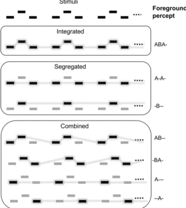
The auditory streaming paradigm (van Noorden, 1975) has been ex- tensively used to study how the human auditory system extracts coherent sound sequences (auditory streams) from a mixture of sounds emit- ted by concurrently active sources (cf. auditory scene analysis; Bregman, 1990). The stimulus is a repeating sound sequence of ABA-ABA-…structure, where“A”and“B”denote two sounds differing from each other in some acoustic features, such as the frequency of simple tones and

“-”stands for a silent interval with the common duration of “A”and

“B” (Fig. 1, top panel). Listeners can perceive this stimulus as a single stream (the integrated percept; Fig. 1, second panel), as two separate streams of isochronous sounds, one for the“A”and another for the“B”sounds (the segregated percept; Fig. 1, third panel), as well as in terms of two streams in which one stream includes some of the“A”

and all of the“B”sounds while the other is made up of the rest of the

“A”sounds (the combined percept; Fig. 1, fourth panel; for a full description of the variants of the combined percept, see Denham et al., 2014). The initial perception of this stimulus is strongly influenced by the stimulus parameters, with larger separation between“A” and“B”

⁎ Corresponding author at: Institute of Cognitive Neuroscience and Psychology, Research Centre for Natural Sciences, Hungarian Academy of Sciences, Magyar tudósok körútja 2, H-1117 Budapest, Hungary.

Email address:farkas.david@ttk.mta.hu (D. Farkas) https://doi.org/10.1016/j.neuropsychologia.2017.11.032

Received 2 February 2017; Received in revised form 15 November 2017; Accepted 27 November 2017 Available online xxx

(2)

UNCORRECTED

PROOF

Fig. 1.Schematic depiction of the auditory streaming paradigm (top panel) and its possible perceptual interpretations grouped into 3 categories (the 3 lower panels). Rectan- gles depict the“A”and“B”sounds with the feature difference between them indicated by displacement in the vertical direction. Time flows along the horizontal direction. Sounds perceived as part of the same stream are connected by lines in the lower panels. Darker rectangles with grey background indicate the stream appearing in the foreground (also described with symbols to the right of each of the lower panels).

and faster presentation rates promoting the perception of the segregated and the opposite the integrated percept (for a review see Moore and Gockel, 2012). However, for longer (>30 s) stimuli, perception in- evitably switches between the alternative percepts (Anstis and Saida, 1985; Bendixen et al., 2010; Deike et al., 2012; Denham and Winkler, 2006; Gutschalk et al., 2005; Pressnitzer and Hupé, 2006) and the effects of the stimulus parameters are reduced at longer delays from the stimulus onset (Denham et al., 2013).

Studies using fMRI have provided information about brain regions activated during perception of the auditory streaming stimulus.^⁠1Audi- tory cortex, especially Heschl's gyrus, is more active when listeners experience the segregated than the integrated sound organization (Wilson et al., 2007). Compatible evidence was obtained with EEG by Snyder et al. (2006), who found that differences between event-related potentials elicited during integrated vs. segregated percepts probably originated from Heschl's gyrus. Deike et al. (2004) found that the left auditory cortex was more active during segregated than integrated perception of the stimulus. However, Cusack (2005) found no difference in auditory cortical activation between the two percepts; rather the intraparietal sulcus was more active during segregation than integration. The latter result is also supported by the data of Kashino et al. (2007), who found that beyond the auditory cortex, the left intraparietal sulcus, the posterior insular cortex, the supramarginal gyrus, and the thalamus were also dif- ferentially involved in the perception of the auditory streaming stimulus. These findings provide evidence that the brain network underlying auditory scene analysis extends beyond auditory cortex.

1 Please note that these studies only took into account the integrated and segregated perceptual alternatives.

Denham et al. (2014) studied individual differences in the perception of the auditory streaming stimulus, characterizing participants’

switching patterns by the conditional probabilities for transitions between perceptual alternatives (Denham et al., 2012). These authors found that although perceptual switching is stochastic, the characteristics of participants' switching patterns tended to be idiosyncratic (switching patterns from the same individual across repeated blocks were significantly more similar in comparison with those of other participants) and stable (individual similarity was preserved across sessions separated by more than a year). Farkas et al. (2016a) identified two main dimensions of the variance in individuals’switching patterns. The first one was termedExploration, because individuals scoring high on this dimension experienced the least frequently reported perceptual alternative (combined) more often and the most frequently reported alternative (integrated) less often, they switched between alternatives more frequently, and required less time to discover all perceptual alternatives compared to those who scored low on the dimension. The second dimension was termedSegregation, because scoring high on the dimension was related to reporting more time spent experiencing the segregated and less the integrated percept (for similar dimensions found in a different group of listeners, see Kondo et al., 2017).

Ego-resiliency (ER; Block, 2002; Block and Block, 1980), a personality meta-trait of adaptive behavioral flexibility was positively linked to theExplorationdimension (Farkas et al., 2016a). Individuals with high ER are able to flexibly coordinate their behavior with situational de- mands in an adaptive way. However, Kondo et al. (2017) did not find a significant relationship between ER and idiosyncratic switching patterns in two auditory multi-stable stimulus paradigms. Discrepancies between the findings of these two studies may stem from the much larger sample size in Farkas et al. (2016a) than in Kondo et al. (2017) study (N= 48 andN= 22). Personality trait related effects typically require larger statistical power due to their higher variability. Further, Kondo et al. (2017) found that the concentration of the glutamate-glutamine (Glx) neurotransmitter measured in auditory cortex was negatively related to theExplorationdimension: higher Glx concentration in auditory cortex accompanied higher proportions of segregated and lower proportions of combined reports. In sum, these correlations between idiosyncratic switching patterns, individual personality traits and neurotransmitter profiles are compatible with the observed temporal stability of switching patterns, as these stable characteristics may influence the perceptual processing of multi-stable auditory stimuli. High creativity has been found to be related to increased switching in ambiguous figures (Doherty and Mair, 2012; Wiseman et al., 2011), but was found to be unrelated to individual differences in auditory streaming (Farkas et al., 2016a). However, there is a lack of consensus both in the definition (Kozbelt et al., 2010) and in the assessment (Plucker and Mackel, 2010) of creativity. Farkas et al. (2016a) study measured creativity using divergent thinking tasks (Torrence, 1988). In the current study, we decided to measure creativity using a self-report scale, as this has been found to provide a better assessment of creativity than divergent thinking tasks (Silvia et al., 2012).

In the current study, we explored the functional brain networks underlying idiosyncratic switching patterns. Functional connectivity refers to the temporal interdependence of the activity of anatomically separate brain regions. In brain networks, functionally separate regions are usually linked with each other through hubs, which integrate information from several regions (Bullmore and Sporns, 2009; Rubinov and Sporns, 2010). The low EEG frequency ranges (delta: 0–4 Hz, and theta:

4–8 Hz) are often thought to predominantly reflect long-distance connections with fewer hubs, whereas, the high frequency ranges (beta:

13–30 Hz, and gamma: 30- Hz) are indicative of short-distance connections with more hubs (Smith-Bassett and Bullmore, 2006). Graphs are used for an abstract mathematical representation of the networks.

A graph is defined as a set of nodes connected with edges. The

(3)

UNCORRECTED

PROOF

Minimum-Spanning Tree (MST) algorithm (Kruskal, 1956; Stam et al., 2014) provides a way to extract the structure of functional networks. A spanning tree is a graph that includes all nodes of the original network (N) linked byN−1 edges and without forming loops. MST graphs can be characterized using metrics representing the network's centrality, connectedness, and modularity.

To date, only one study has examined functional networks (though not functional connectivity in the above defined sense) in the auditory streaming paradigm (Kondo and Kashino, 2009). Connections between regions of interests (ROI) were calculated by Structural Equation Mod- eling (SEM) of event-related fMRI activity time-locked to perceptual switches. The left and right auditory cortices (AC) were strongly correlated and the right AC was also correlated with the right medial genic- ulate body (MGB). Further, the right MGB was correlated with the left cerebellar area. Comparing these connections between two groups differing in the number of switches, the authors found generally stronger connections in the group with more frequent perceptual switching, especially for the connection between the right AC and MGB. Thus, it appears that the AC-MGB loop is an important generator of switches between alternative perceptual organizations.

We hypothesized that the main dimensions found to explain the perceptual variability of individuals for auditory streaming stimuli (Farkas et al., 2016a; Kondo et al., 2017) are supported by different functional brain networks. Because some previous studies found associations between inter-individual variability in perceiving multi-stable stimuli and some personality (ego resiliency and creativity) and executive function measures (performance in the Stroop task and semantic fluency), find- ing separate functional brain networks associated with the perceptual dimensions would provide important links between these different lev- els of description of human behavior. Finally, based on the notion that integration may be assumed to be the default mode of sound organization (Bregman, 1990), one could theorize that integration would be subserved by more local networks than the other sound organizations.

2. Material and methods 2.1. Participants

Sixty volunteers without a history of psychiatric or neurological dis- orders (32 female; 18–37 years of age;M = 22.78,SD = 3.15; 53 right-handed) participated in the experiment. During the experimental session, they performed a perceptual task during which EEG and near-infrared spectroscopic (NIRS) signals were recorded from the scalp, performed tasks assessing some executive functions, and filled personality questionnaires (see details in Section 2.2). All participants had pure-tone thresholds within normal limits for the frequencies ranging from 250 Hz to 4 kHz: none exceeded the normal hearing threshold by more than 25 dB in either ear and none had more than 10 dB threshold difference between the two ears. Participants gave written informed consent after the aims and methods of the study were explained to them. The study was conducted in full accordance with the Helsinki Declaration and all applicable national laws and it was approved by the inter-University Ethical Review Committee for Research in Psychol- ogy (EPKEB). Participants received modest financial compensation. Five participants did not pass the training procedure: they did not reach 80% correct responses by the end of the training (see section Audi- tory perceptual task). One participant's data was excluded due to NIRS data recording errors. Another participant's data was excluded due to reporting far more‘none’ responses (25%; see section Auditory perceptual task) compared to the rest of the group (1%), which made her Grubb's outlier detectionz-score 5.5, almost double the acceptable maximum (3). Finally, eleven participants’ data were excluded from the analysis based on poor performance (<60%) in the catch-trials,

which were appended to each stimulus block (see section Auditory perceptual task). Thus, the final sample consists of 42 participants (23 female; 19–37 years of age;M= 23.10,SD= 3.41; 40 right-handed).

2.2. Measurements

2.2.1. Auditory perceptual task

Sinusoidal tones of 75 ms duration with 10 ms rise and 10 ms fall times were presented in the auditory streaming paradigm (a cyclically repeating„ABA-”pattern; Fig. 1, top panel). The frequency difference between the “A” and “B” tones was 4 semitones with the „A” tone frequency set at 400 Hz and“B”tone at 504 Hz. The stimulus onset asynchrony (SOA, onset-to-onset interval) was 150 ms and the intensity was 45 dB sensation level; individual hearing thresholds were separately measured for each participant using a staircase procedure with the sounds employed in the experiment. Participants were presented with nine four-minute-long sequences of the auditory streaming stimulus with an additional ca. 40 s catch-trial segment (see the Proce- dure section) appended without a break to the end of each stimulus.

Tones were delivered through Sennheiser HD600 headphones by an IBM PC computer using Psychtoolbox-3 (Brainard, 1997; Pelli, 1997) under MATLAB 2015b (Mathworks, 2015).

Listeners were instructed to mark their perception continuously in terms of four possible categories using two response keys: a) „integrated”(ABA-; Fig. 1, second panel; response: depressing one of the two response keys), b)„segregated”(A-A-/B—; Fig. 1, 3rd panel; depressing the other response key), c)„combined”(-AB-/—A or -BA-/A; Fig.

1, bottom panel; simultaneously depressing both response keys), and d)

„none”(no repeating pattern perceived; releasing both response keys).

Note that, similarly to the integrated and the segregated percept, the combined percept appears spontaneously when listening to sequences of the auditory streaming paradigm (Denham et al., 2013). Participants received instructions and training for identifying the different perceptual categories without hesitation. They were instructed to report faithfully their perception as it occurred. The description of the integrated percept emphasized hearing all tones as part of a single repeating pattern with a galloping rhythm. The description of the segregated percept emphasized hearing two isochronous sound streams in parallel, one in the foreground, the other in the background, each with a uniform (one slower, the other faster) delivery rate. The description of the combined percept emphasized the perception of two parallel streams of sound, at least one of which included a repeating pattern composed of both high and low tones. Finally, the“none”choice allowed listeners to indicate that they did not hear any repeating pattern or could not decide between the patterns previously described to them. Participants were instructed to maintain the key combination depressed for as long as they continued hearing the corresponding pattern and to switch to another combination as soon as their perception changed. They were informed that there was no“correct”response and asked to employ a neutral listening mind-set (termed“neutral instructions”; for an in-depth discussion of the instructions, see Denham et al., 2013). The left and right arrow keys of a stan- dard Hungarian IBM PC keyboard were used as response keys with their roles counterbalanced across participants. The state of the response keys was continuously recorded at a sampling rate of 10 Hz.

Training started with the participant listening to six one-minute long demonstration sequences, each promoting the perception of one of the alternatives shown in Fig. 1. The integrated percept was introduced by using a smaller frequency difference between the„A”and „B” tones than the parameters chosen for the experiment (1ST; 400 and 426 Hz, respectively); the segregated percept was initially demonstrated by using a larger frequency difference (890 Hz). Subsequently, the two segregated and the three combined percepts (as shown in Fig. 1.) were

(4)

UNCORRECTED

PROOF

demonstrated by emphasizing the corresponding repeating tone pattern within the auditory streaming sequence used in the experiment. Empha- sis was created via attenuating by 18 dB those tones which were part of the intended background stream; further, the timbre of these tones was changed to a complex tone with eight harmonics of equal intensity. These demonstrations promoted perception of the normal-intensity pure tones as a coherent foreground stream. After the response key as- signment and the„none”choice were explained, training continued in blocks of six sequences separated by short silent intervals. The first sequence was one-minute-long and its parameters were identical to those used in the experiment. This was followed by five sequences of 6–9 s, one for each of the percepts the participant was required to identify.

These short segments served as catch trials. The order of the five short sequences (the small-frequency-difference and the four attenuated-intensity variants of the auditory streaming stimulus) was randomized separately for each training block. Training was completed when the participant made the expected response in at least 80% of the presentation time during the catch trials or when 10 training blocks had been delivered. During the training blocks, the experimenter gave feedback and further help as needed. Five participants were rejected on the basis of their performance in the training blocks.

Catch trials of the same structure were appended to each stimulus block in the main experiment, allowing the monitoring of the participants’understanding of the instructions throughout the experiment.

Participants who scored lower than 60% in the catch segments, aver- aged across all stimulus blocks, were excluded from the data analysis.

Eleven participants’data was excluded in this way, as noted in the previous section.

2.2.2. Pre-processing perceptual data

Perceptual phases (continuous intervals with the same combination of response keys depressed) were extracted from the key press records.

Phases shorter than 300 ms were discarded, because these were assumed to result from finger coordination misalignments during switching between key combinations (see Moreno-Bote et al., 2010). The data removed this way amounted to ca. 0.4% of the total duration.

Transition matrices, containing conditional probabilities for transitions between perceptual alternatives, were constructed from the perceptual reports using the method described in Denham et al. (2012).

Transition matrices had 4 rows and 4 columns (each corresponding to one of the 4 alternative perceptual choices described above) with cells representing the conditional probability of the percept changing from the starting percept (column) to the percept assigned to the row; the di- agonal contained the probability of no change. The conditional probabilities were estimated for each listener and stimulus block, separately (block transition matrix), for each listener (by pooling data from all stimulus blocks of a listener: listener transition matrix), and for the whole experiment (by pooling data from all blocks and participants:

global transition matrix). Denham et al. (2012) showed that the global transition matrix can be used to optimally estimate missing data (i.e., unobserved transitions) for individual listeners while listener transition matrices can be used for estimating missing data in the individual's block transition matrices. This procedure was employed for substituting missing data. Because the switching patterns obtained in the very first stimulus block were shown to substantially differ from those obtained in subsequent blocks (Farkas et al., 2016b), data from the first block were excluded from the analyses. Four listeners never experienced the combined percept. On average, 31.9% of the sixteen possible transitions were missing within the block transition matrices. Most of the missing transitions were related to the„none”percept, whose overall proportion was less than 0.62% in the data. Since we did not analyze the„none”

responses, the effective proportion of missing transitions was 13.19%.

Similarly to previous studies investigating individual differences in perceptual multi-stability (e.g., Farkas et al., 2016a), the mean number of switches between the alternative perceptual reports, and the proportions and mean phase durations of the integrated, segregated, and combined perceptual reports were entered into the statistical analyses.

These variables were extracted from the listener transition matrices. The time to discover all three perceptual alternatives was added to the above list of variables as it provides information about the viability of the alternative percepts for the listener. Short discovery times suggest that all alternatives were relatively easy to discover for the given listener, whereas long discovery times suggest that some perceptual alternatives were less accessible to him/her. The discovery time for each participant was determined by simulating the switching behavior of the listener 1000 times, based on the listener's transition matrix. In each run, the simulation stopped when all patterns had been discovered. The value for the time to discover all patterns was defined as the median of the values from the simulation runs.

2.2.3. EEG recording and preprocessing

EEG was recorded with a BrainAmp DC 64-channel system with act- iCAP active electrodes. The electrodes were placed according to the In- ternational 10/20 system (Fig. 2) with an additional electrode attached to the tip of the nose. Bipolar recording from two further electrodes, one attached lateral to the outer canthus of the right eye and the other below the left eye, was used for monitoring eye movements. During recording, the FCz electrode served as the common reference. Sampling rate was 1 kHz, and a 100 Hz online low-pass filter was applied. The electrode impedances were kept below 20 kΩ.

The continuous EEG signals recorded from the second to the fifth stimulus block were re-referenced to the average voltage of all electrodes and filtered between 0.5–45 Hz^⁠2by a finite impulse response (FIR) band-pass filter (Kaiser windowed; Kaiserβ= 5.65; filter order 1812) by the EEGlab 11.0.5.4.b toolbox (Delorme et al., 2007) under Matlab 2015b (Mathworks, 2015). A maximum of one malfunctioning EEG channel per participant was interpolated using the spline interpo- lation algorithm implemented in EEGlab. The Infomax algorithm of In- dependent Component Analysis (ICA) of EEGlab was employed for ar- tifact removal (for detailed mathematical description and validation, see Delorme et al., 2007). ICA was performed on the continuous filtered dataset of each participant, separately. ICA components consti- tuting blink artifacts were removed via visual inspection of their topo- graphical distribution and frequency content. Due to the high compu- tational demand of EEG source analysis, epochs of 2048 ms duration were extracted from the preprocessed signals. Epochs with an amplitude change exceeding 100μV at any electrode were rejected from further analysis. The final dataset consisted of minimum of 376 epochs (M= 452.19,SD= 18. 37) per participant.

EEG sources were reconstructed using the minimum norm estimate model (sLORETA developed by Pascual-Marqui, 2002 based on Hämäläinen and Ilmoniemi, 1994) included in the Brainstorm toolbox (Tadel et al., 2011). Using the MNI system, the generic anatomical brain template was segmented into 15002 voxels with a resolution of 1×1×1 mm restricted to lie within the grey matter. Default electrode locations were entered into the forward model provided by the open- MEEG algorithm (Gramfort et al., 2011). Note that individual variance in head shape and electrode placement was not taken into account. The time-varying source signals were modeled wherever the dipole had a component perpendicular to the cortical surface. By averaging all di

2 The EEG data was reanalyzed using a 80 Hz low pass filter and a 47–53 Hz notch filter assessing the higher (>55 Hz) gamma band. As this analysis did not yield results relevant for the main conclusions, it can be found in Supplement 2: 30–80 Hz gamma band analysis.

(5)

UNCORRECTED

PROOF

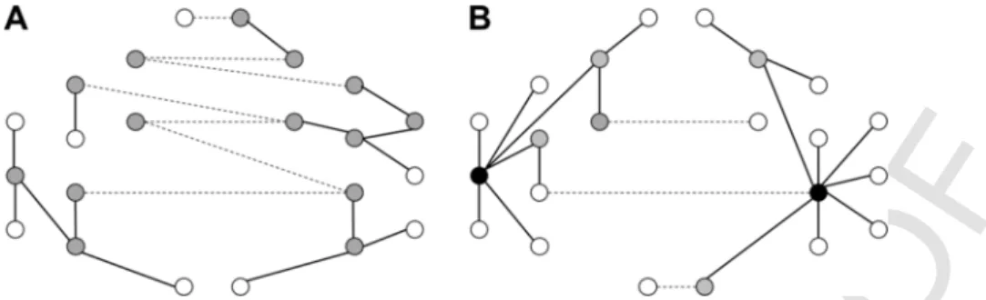
Fig. 2. Examples of two different MST graphs based on the schematic configuration.All dots depict nodes. Empty dots depict peripheral nodes, grey dots depict nodes that have at least two connections, whereas black dotes depict nodes having more than three connections (centers or hubs). Lines depict edges, whereas dashed lines depict interhemispheric edges.

Subplot A depicts a decentralized MST with no centers, a few peripheral nodes, and many interhemispheric connections. Thus, this network would have a low leaf fraction, a low tree hierarchy, and a high number of interhemispheric connections. Subplot B depicts a more centralized network with two hubs, many peripheral nodes and a few interhemispheric connections.

Thus, this network would have a high leaf fraction, a high tree hierarchy, and a low number of interhemispheric connections.

pole strengths of the voxels in the corresponding cortical regions, the mean neuronal activity (current density) was derived for 62 cortical regions using a parcellation scheme (Klein and Tourville, 2012) set prior to the analysis. The number of connections in functional networks grows exponentially with the number of nodes used to create them, and having a large number of edges increases the probability of false positive connections. Thus, some of these cortical regions were excluded from further analysis after the source analysis procedure. Occipital regions were excluded from further analysis, because they are unlikely to be involved in auditory streaming. Motor areas were excluded, because the participants’constant button pressing would have likely produced connections unrelated to auditory streaming. In sum, 15 cortical regions per hemisphere were excluded, leaving 16 cortical regions of interest (ROI) per hemisphere (Table 1) for further analysis.

The goal of source localization was to investigate the interplay between brain regions during perception of the auditory streaming stimulus and relate this interplay to inter-individual variance in perception. However, due to the lack of individual MRI scans and electrode localization data, the current source analytical protocol does not al- low a sufficiently precise localization of EEG sources for reliably distin- guishing any pair of the 16 regions per hemisphere. A likelihood analysis (based on the studies of Baillet et al., 2001; Huang et al., 2016;

Pizzagalli, 2007; Plummer et al., 2008; Song et al., 2015) conducted with the assumption of a 1.5 cm leakage distance and 50% overlap criterion showed only one case of significant overlap: the transverse temporal gyrus can overlap with the superior temporal and supramarginal

Table 1

Regions of interest (ROI) per hemisphere and their abbreviations.

Region of interest Abbreviation Brain regions

Superior Frontal Gyrus SFG Frontal regions

Medial Orbitofrontal Gyrus OFG med Caudal Middle Frontal Gyrus MFG caud Rostral Middle Frontal Gyrus MFG rost Opercularis Inferior Frontal

Gyrus IFG operc

Parsorbitalis Inferior Frontal

Gyrus IFG orb

Triangularis Inferior Frontal

Gyrus IFG triang

Caudal Anterior Cingulate

Gyrus ACG caud Anterior Cingulate

regions Rostral Anterior Cingulate

Gyrus ACG rost

Inferior Temporal Gyrus ITG Temporal regions

Middle Temporal Gyrus MTG

Superior Temporal Gyrus STG

Transverse Temporal Gyrus HES

Supramarginal Gyrus SMG Parietal regions

Inferior Parietal Gyrus IPG

Superior Parietal Gyrus SPG

regions. Despite this issue, we decided to employ the above described parcellation, because by using a coarser resolution and thus collapsing large chunks of data would have eliminated a large part of inter-individual differences existing in the data, the primary goal of the study.

However, acknowledging that the resolution of parcellation is higher than what is allowed by the data, the high-resolution current source analysis is only used for functional network formation and visualization, thereby allowing the exploration of variance in the network structure.

In contrast, interpretation of the findings is expressed in terms of much broader brain regions, as specified in Table 1 (right column).

Source signal epochs were re-merged into a single time-series, separately for each participant for compatibility with the behavioral data, which was analyzed using continuous time series. These signals were then filtered using band-pass finite impulse response (FIR) filters (Kaiser windowed, Kaiserβ= 5.65, filter order = 1812) into six EEG bands:

delta (.5–4 Hz), theta (4–8 Hz), lower alpha (8–10 Hz), upper alpha (10–13 Hz), beta (13–30 Hz), and gamma (30–45 Hz). Undirected functional connectivity matrices were calculated separately for the EEG bands and participants by measuring phase synchronization strength between all pairs of EEG source ROIs using the phase lag index (PLI; Stam et al., 2007). PLI calculates the asymmetry of the phase difference distribution between two signals, and reflects the consistency with which one signal's phase leads or lags that of the other. This resulted in 32*32 functional connectivity matrices (16 ROI×2 hemispheres), separately for each participant and EEG frequency band.

2.2.4. NIRS recording and other measures

NIRS signals were recorded with a montage of 16 sources and 24 de- tectors by the NIRStar 14.1 device (NIRx Medical Technologies, 2014).

Because the results obtained from the analysis of this data did not significantly contribute to the report, the methods and results related to the NIRS data can be found in Supplement 3: Near-Infrared Spectroscopy (NIRS) analysis.

Two executive functions were assessed: The inhibition executive function was measured using the Stroop task (Lansbergen et al., 2007;

Stroop, 1935) and the shifting executive function was assessed by semantic fluency (Troyer et al., 1997). Participants filled out two questionnaires: The ER89 questionnaire (Block and Kremen, 1996), which measures ego-resiliency (ER) and theBiographical Inventory of Creative Behaviors(BICB, Batey, 2007), which measures creative achievements.

The details of these measures and their analysis are described in Supplement 1: Executive functions, questionnaires, and correlation analysis.

2.3. Procedure

The experimental session started with filling out the questionnaires and measuring the executive functions. The order of the questionnaires

(6)

UNCORRECTED

PROOF

was fixed (ER89 followed by BICB), whereas the order of the executive function tasks was counterbalanced across participants. This was followed by the auditory perceptual task, which consisted of the training part followed by 9 experimental stimulus blocks. After the training, participants were fitted with the EEG electrodes and NIRS optodes. They then completed one further training block before starting the main experiment.

During the first five stimulus blocks, participants reported their perception according to the neutral instructions described in the“Auditory perceptual task section”(Neutral condition). For two of the remaining four blocks, participants were instructed to hold on to each percept for as long as they could (Hold condition) while still reporting their perception faithfully. For the other two blocks, participants were instructed to switch to another percept as soon as they could (Switch condition) while also marking their perception truthfully. The order of these two bi- ased conditions was counterbalanced across participants. Only the data recorded using the neutral instructions are reported here. Breaks were included when switching between tasks and between blocks as needed.

The session lasted for ca. 180 min.

2.4. Data analysis

MATLAB 2015b (Mathworks, 2015) was used for all data analysis.

2.4.1. Idiosyncratic switching patterns

Intra-individual similarities of switching patterns were calculated using the Kullback-Leibler (K-L, Kullback, 1959) distance between each pair of the block transition matrices of the same listener. Inter-individual similarity was assessed by calculating the K-L distances between block transition matrix pairs for each combination of pairs of blocks from two different listeners. Separately for each listener, the two measures were compared using a one-tailed Wilcoxon's Signed Rank test.

When intra-individual similarity was significantly lower than inter-individual similarity for the same listener the listener was categorized as having an idiosyncratic switching pattern.

2.4.2. Multi-dimensional scaling of the individual switching patterns Based on the inter-individual K-L distances of the listener transition matrices, Multi-Dimensional Scaling (MDS, Kruskal and Wish, 1978) was set up to find the main dimensions characterizing listeners’perceptual switching behavior in the auditory streaming paradigm. MDS uses the distances between data points to extract the dimensions explaining the variance of the data.“Stress values”(Kruskal and Wish, 1978) assess how well the observed distance matrix is reproduced by a given MDS configuration. A linear stress criterion was used as an index of the good- ness-of-fit, which is the stress value normalized by the sum of squares of the inter-response distances. The number of dimensions was determined using the scree test (Cattell, 1966), which evaluates the stress values for different MDS solutions.

2.4.3. Functional network construction and network metrics

The Minimum Spanning Tree (MST; Kruskal, 1956; Stam et al., 2014) algorithm was used for a topological representation of the structure of the functional connectivity matrices. MST is a method to con- struct a graphical representation of a network in which all nodes are connected to each other without forming circles or loops. MST networks were derived for each participant. Only those edges which were most often present, i.e. the top 5%, in participants MST network (based on the edge MST connection distributions) are shown in the figures.

Edge selection for visualization had no effect on the variables calculated from the MST metrics. These are shown on circular graph plots based on the Matlab function developed by Paul Kassebaum (http:

//www.mathworks.com/matlabcentral/fileexchange/48576-

circulargraph) and on the cortical surface using the BrainNet Viewer (Xia et al., 2013).

MST functional networks were characterized by the following three derived measures. 1)“Leaf fraction”gives an estimate of how much pe- riphery a network has by dividing the number of nodes with only one connection by the total number of nodes. A high leaf fraction value indicates a graph with a few centers and many peripheral nodes. 2)“Tree hierarchy”provides an estimate of how hierarchical a network is by the normalized rate of the number of connections per node. Low tree hierarchy values indicate non-hierarchical networks with no distinct centers, whereas high values indicate centralized, hierarchical networks.

3) Finally, the number of interhemispheric connections was calculated.

Examples for MST graphs with different characteristics based on these measures are depicted in Fig. 2.

2.4.4. Correlation analysis

Measures originating from different methods were grouped into categories: perceptual measures (8), questionnaire measures (3), executive function measures (3), and graph metrics measures (three graph metrics with the six EEG frequency bands: 18). MDS dimensions were interpreted by correlating them with the perceptual measures. Because some of the variables did not have a normal distribution, and a nor- mality transformation could have distorted their magnitude, Spearman's rank-order correlations were used. Family-wise error was controlled by a permutation method: the distribution of the absolute values of the correlation coefficients under the null hypothesis was estimated by permut- ing the values of all perceptual variables and correlating them with the given MDS dimension 10,000 times. In each permutation run, the highest absolute correlation coefficient was registered. The distribution of the maximal coefficients was used to establish the p-value of the observed correlation as the proportion of the random correlations higher than or equal to the observed value (cf. Farkas et al., 2016a). Both the empirical and family-wise error corrected (marked asp_⁠fwe)p-values are reported.

3. Results

3.1. Idiosyncratic switching patterns and multi-dimensional scaling Based on the K-L distances between transition matrices, 37 of 42 listeners (88.1%) showed significantly higher intra-individual than inter-individual similarity, suggesting that they had an idiosyncratic switching pattern (for the individual results see Supplement 4: Table 1).

The scree test indicated that two dimensions were sufficient for de- scribing the transition matrix space of the listeners' switching patterns (MDS stress = .049). The first MDS dimension was positively related to the proportion of the combined percept reports (r(42) = .992,p<

.001,p⁠fwe< .001) and to the number of switches (r(42) = .464,p= .002,p_⁠fwe = .016). It was negatively related to the proportion of the integrated percept (r(42) = −.652,p< .001,p_{⁠fwe <}.001), to the duration of the segregated percept (r(42) = −.477,p= .001,p⁠fwe= .010), and to the time to discover all perceptual alternatives (r(42) = −.683, p< .001,p_⁠fwe< .001). This pattern of correlations indicates that participants with high values on this dimension switched more often, required less time to discover all perceptual alternatives, reported segregation for shorter phase durations, and experienced the integrated percept for lower and the combined percept for a higher proportion of the time compared to participants scoring low on this dimension. We term this MDS dimensionExploration. The second MDS dimension was positively related to the proportion (r(42) = .675,p< .001,p⁠fwe< .001) and the duration of the integrated percept (r(42) = .507, p= .001, p_⁠fwe= .004), whereas it was negatively related to the proportion of the segregated percept (r(42) = −.887,p< .001,p⁠fwe< .001). This correlation pattern suggests that the second dimension separates partici

(7)

UNCORRECTED

PROOF

pants who reported more integration and less segregation from those with the opposite balance between these two percepts. We term this di- mensionSegregation. We also noted that segregation was reported first in 10.71% of the stimulus blocks, and the combined pattern in 8.33%

blocks. In the remaining stimulus blocks, the integrated percept was reported first.

3.2. Functional networks

The functional connections appearing most often (top 5%) in the listeners’ MSTs are shown in Fig. 3, separately for the six EEG frequency bands. In thedeltaband, the left ITG has the highest number of connections (i.e., serving as a hub), predominantly with frontal regions. Temporo-parietal networks are indicated in both hemispheres, whereas in the left hemisphere, fronto-temporal connections are also present. In thethetaband, the left SMG shows connections with both frontal and caudal regions. Left temporal regions, especially the ITG and STG display both frontal and caudal connections, including some interhemispheric ones. The right hemisphere shows a similar pattern, but with lower number of connections. In thelower alpha band, the number of frontal and caudal connections is lower, while temporo-parietal connections are more common compared to the delta and theta bands. Left temporal and both parietal regions appear to have the highest number of connections. In theupper alphaband, parietal regions become even more prominent compared to the lower frequency bands, and the number of frontal connections further decreases. Thebetaband is characterized by shorter, predominantly temporo-parietal connections, and no inter-hemispheric connections are present. The gamma

band connections remain local as was observed for thebetaband, but the connection density shifts back from parietal to frontal regions.

In sum, the lower frequencies show more inter-hemispheric connections and hubs in the temporal, especially the left temporal, regions. Moving from lower to higher frequency bands, the number of inter-hemispheric connections decreases, and networks become less centralized. Further, graphs from the lower frequency bands show more fronto-temporal connections, whereas temporo-parietal connections become more prominent in higher frequency bands.

3.3. Correlation with the EEG measures

Some of the graph metrics of the functional networks for the six different EEG bands showed significant relationships with some measures characterizing switching in the auditory streaming paradigm as well as with some executive functions. Results from the theta band functional network graphs suggest that interhemispheric connections within this band are positively related to theSegregationdimension of the MDS (r(42) = −.418,p= .006,p⁠fwe= .019) and also consistently correlated with all of the perceptual measures associated with this dimension (see the Section“Idiosyncratic switching patterns and multi-dimensional scaling”). Higher numbers of interhemispheric connections result in larger proportion of segregation (r(42) = .388, p= .011, p_⁠fwe = .035) and lesser proportion (r(42) = −.388,p= .011,p_⁠fwe= .033) and shorter average phase duration of integration (r(42) = −.494,p

= .001, p⁠fwe = .003). Further, more hierarchical networks are associated with higher scores in the shifting executive function, namely higher tree hierarchy was associated with lower cluster sizes (r(42) =

Fig. 3. Functional connections appearing most often (top 5%) in the listeners’Minimum-Spanning Tree graphs for the six EEG bands.From upper left to lower right, panels represent functional connectivity in the delta, theta, lower alpha, upper alpha, beta, and gamma bands. Each panel contains visualization of the edges on three plots of the cortical surface (top, left, and right view), where dots represent the spatial locations of the EEG sources reconstructed for the 16 ROIs (nodes in the graphs) in MNI space. The size of the dot represents the number of connections of the ROI. Edges are also shown on abstract circular graphs. The left and right sides of the circle represent the two hemispheres. The color of the ROI dots (for abbreviations, see Table 1) indicates the lobe (the unit of interpretation): red–frontal, yellow–cingular, green–temporal, blue–parietal. (For interpretation of the references to color in this figure legend, the reader is referred to the web version of this article.)

(8)

UNCORRECTED

PROOF

−.390,p= .011,p_⁠fwe= .035) and higher leaf fraction was associated with increased number of switches between categories (r(42) = .454,p

= .003,p⁠fwe= .009)

Graph metrics of both of thealphaand thebetaband were related to theExplorationdimension of the MDS. For the loweralphaband, more connections between the two hemispheres is related to higher values inExplorationdimension of the MDS (r(42) = .375,p= .014,p⁠fwe= .041) and a larger proportion of the combined percept (r(42) = .371, p= .016,p_⁠fwe= .044), which is a correlate ofExploration. Correlations found between MST measures for the higheralpha(r(42) = .384,p= .012,p⁠fwe= .037) andbeta(r(42) = .385,p= .012,p⁠fwe= .037) bands and perceptual measures suggest that functional networks with a higher percentage of peripheral nodes (more centralized networks) are accompanied by longer times for discovering all perceptual patterns, which is negatively related toExploration. In the upperalphaband, the percentage of peripheral nodes of the MST was also positively related with the average phase duration of the integrated percept (r(42) = .383,p

= .012,p_⁠fwe= .035) and negatively with inhibition in the Stroop task (r(42) = .381,p= .013,p⁠fwe= .038).

4. Discussion

The aim of the current study was to test whether the two main dimensions explaining inter-individual variance in perceiving auditory streaming stimuli are associated with different functional brain networks. The proportion of participants with idiosyncratic switching patterns was similar to that reported by Farkas et al. (2016a). The main dimensions of the switching patterns—ExplorationandSegregation—were the same as the ones previously found by Farkas et al. (2016a) and similar to the those observed by Kondo et al. (2017), and showed very similar patterns of correlations with perceptual measures as the ones found in these previous studies. Functional networks derived from the EEG data suggest that these perceptual differences are accompanied by different functional connections in the brain.

Based on these results, it appears that the main dimensions of individual differences in auditory streaming are quite consistent. That is, listeners’experience of auditory streaming can be largely described by two dimensions. The first, one is the tendency to explore the environment and the second is the tendency to perceptually segregate versus integrate incoming sound events. The observed EEG functional connectivity as a function of frequency band is compatible with the assumed functional role of low- and high-frequency oscillatory networks in the brain (Smith-Bassett and Bullmore, 2006): power in lower frequency bands may reflect the integration of information across anatomically distant areas and they connect through a few hubs, whereas higher frequency bands are probably associated with short-distance connections mediated by a larger number of hubs. Note that the border between low and high frequency bands varies in the literature. Here we only regard delta and theta as low-frequency oscillations. In the lower frequency bands, we found functional networks with the hubs often located in left temporal areas. These regions displayed several connections to anatomically distinct areas as well as many interhemispheric connections. In both alpha bands, there are long-range as well as local connections. Parietal regions were often involved within these networks. In the two higher frequency bands (beta and gamma), local connections were more typical.

Characteristics of each frequency-band network were linked with the individuals’experience of listening to the auditory streaming stimulus. The number of interhemispheric connections in the theta networks correlated with the perceptual dimension Segregation: partici- pants who reported segregation more than integration were characterized by a larger number of interhemispheric connections than those who reported more integration. The number of interhemispheric connections observed for the lower alpha-band networks, was related to

higher incidence of the combined pattern and higher scores on the Exploration dimension. Together, these results suggest that networks mainly located in left auditory areas underlie the perception of integration, whereas perceiving the alternative patterns is accompanied by stronger interhemispheric connections. A major difference between segregated and combined is that they are associated with networks operating over different EEG frequency bands. Whether this separation is due to more complex temporal-spectral organization of the combined compared to the segregated percept or to some other reason cannot be de- duced from the current data.

The current data has implications for how one can conceptualize the build-up of auditory streams. Traditionally, it has been assumed that integration is the default mode of auditory processing in stream segregation and that it requires time to build-up separate streams (Anstis and Saida, 1985; Bregman, 1990), although this assumption has been chal- lenged (Deike et al., 2012; Denham et al., 2013). The current data is incompatible with the assertion that a default mode of the auditory system processes sound sequences in terms of the integrated organization, because in close to one-fifth of the experimental blocks, integration was not the first reported percept. The current data suggests that whereas integration appears as a default tendency within (left) auditory cortical areas, depending on the strength of inter-regional communication, the initial perception of a sequence may also be different. That is, integration is not the default for the whole perceptual system.

The results also provide evidence that the combined percept is in- deed a distinct perceptual alternative. Historically, the combined percept has not been considered, and to now, only behavioral evidence sup- ports that it is separate from the two main (segregated and integrated) alternatives (Denham et al., 2013, 2012, 2014; Farkas et al., 2016a, 2016b; Kondo et al., 2017). The current data shows that the perception of the combined pattern is associated with stronger connections in a different frequency band than perception of the segregated pattern. Thus, these results suggest that combined and segregated perceptual patterns are characterized by different neural processes and thus they should be distinguished in behavioral studies.

The upper alpha and beta frequency band network graphs were related to theExplorationdimension. In both of these frequency bands, the time required to discover all patterns was related to the leaf fraction of the graphs. This indicates that individuals with fewer peripheral nodes explore the auditory environment faster than those who have more. Fewer peripheral nodes in a minimum-spanning tree graph suggests that the number of possible edges is distributed more uniformly across nodes, making the graph more decentralized and interconnected.

Thus, this result can be interpreted as suggesting that when brain regions are more interconnected (in the upper alpha and beta bands), the exploration of alternative patterns proceeds more quickly. Further, in the upper alpha band, the presence of a larger number of peripheral nodes was also related to increased average phase duration for the integrated percept. Given that the integrated pattern is reported initially in over 80% of the stimulus blocks, this result probably reflects the longer time needed to discover all perceptual patterns.

Taken together, the correlations found between EEG functional network parameters and perceptual variables indicate that the main dimensions explaining the variance of the individuals’switching behavior are indicative of functionally distinct processes in the brain: the perceptual dimensionSegregationis linked with some characteristics of theta-band networks andExplorationwith lower- and upper-alpha and beta-band networks. Further, the two most prominent constituents of theExplorationdimension, the proportion of the combined responses and the time needed to discover all patterns, were also linked with network characteristics in different frequency bands. Thus, constituents of the Explorationdimension are associated with different frequency bands, which suggests that they are subserved by separate processes.

Whereas some constituents of the current Exploration dimension are

(9)

UNCORRECTED

PROOF

tied to the auditory streaming paradigm (such as the proportions and phase durations of the specific percepts), others can be used to generally characterize perception in complex scenes (such as the time to discover all patterns and the frequency of switching between alternative percepts). The different functional networks associated with these measures may reflect that the currentExplorationdimension is related to a more general tendency for exploration in individuals, which is colored by the actual stimulus paradigm used to capture it.

Limitations of the current study mainly concern the source reconstruction of the EEG data. Source reconstruction gives a statistical solu- tion to the inverse problem concerning the sources of EEG signals, thus the data from this analysis is only a model of the likely origin of the observed signals. This model can be improved by constraining the analytical procedure with additional information. MRI scans and electrode localization data could increase the validity of this estimation. However, we were not able to obtain this information. A further limitation con- cerns the functional network construction using the functional connectivity matrices. The Minimum Spanning Tree (MST, Kruskal, 1956; Stam et al., 2014) method is fully automatic and data-driven. An advantage of this is that network construction is not based on haphazard choices of the threshold above which the most important edges are selected.

Due to the lack of previous functional network analysis studies of the auditory streaming paradigm with EEG, this method seemed an appro- priate choice for this study. However, this approach removes any possi- bility to parametrize the procedure based on theoretical considerations.

It should also be noted that MST creates functional networks without forming loops within the graph. While this enables the use of well-defined graph metrics, which were instrumental in the current study, it is possible that some important local networks or well-connected regions are missed using this method.

In conclusion, these results show that listeners’ perception of the auditory streaming paradigm is idiosyncratic and the main dimensions on which they differ from each other,ExplorationandSegregation, are linked to different functional brain networks. The theta frequency band is related toSegregationand its constituents, whereas the alpha and beta frequency bands were found to be related toExplorationand its constituents. It seems that a key factor for perceiving the segregated and combined percepts lies in the connectedness between the left auditory cortex and the right–hemispheric regions. The centralized vs. decentralized nature of the upper alpha- and beta-band networks were linked with the time to discover all patterns and the number of perceptual switches. Thus, listeners’idiosyncratic switching behavior during auditory streaming can be described by behaviorally observed dimensions which are rooted in distinct patterns of functional connectivity in the brain.

Uncited references

;.

Acknowledgements

We thank Zsuzsanna Kocsis for help with the independent component analysis of EEG and Dr. Brigitta Tóth for help with EEG preprocessing, source analysis, and functional connectivity analysis. The authors thank Zsuzsanna D′Albini, Zsuzsanna Kovács, and Botond Ha- jdu for their help in running the experiment. This research was supported by the Hungarian Academy of Sciences (Lendület Project LP-36/

2012 to DF and IW). and by the EU Seventh Framework Programme (FP7-PEOPLE-2013-ITN-604764 to SD)

Appendix A. Supporting information

Supplementary data associated with this article can be found in the online version at doi:10.1016/j.neuropsychologia.2017.11.032.

References

Aafjes, M., Hueting, J.E., Visser, P., 1966. Individual and interindividual differences in binocular retinal rivalry in man. Psychophysiology 3, 18–22.

Anstis, S.M., Saida, S., 1985. Adaptation to auditory streaming of frequency-modulated tones. J. Exp. Psychol. Hum. Percept. Perform. 11, 257–271. https://doi.org/10.1037/

0096-1523.11.3.257.

Baillet, S., Riera, J.J., Marin, G., Mangin, J.F., Aubert, J., Garnero, L., 2001. Evaluation of inverse methods and head models for EEG source localization using a human skull phantom. Phys. Med. Biol. 46, 77–96. https://doi.org/10.1088/0031-9155/46/1/306.

Batey, M.D., 2007. A psychometric investigation of everyday creativity, Doctoral disserta- tion. University of London.

Bendixen, A., Denham, S.L., Gyimesi, K., Winkler, I., 2010. Regular patterns stabilize auditory streams. J. Acoust. Soc. Am. 128, 3658–3666. https://doi.org/10.1121/1.

3500695.

Block, J., 2002. Personality as an Affect-processing System: Toward An Integrative Theory.

Psychology Press, Oxford, UK.

Block, J., Kremen, A.M., 1996. IQ and ego-resiliency: conceptual and empirical connections and separateness. J. Pers. Soc. Psychol. 70, 349–361. https://doi.org/10.1037/

0022-3514.70.2.349.

Block J.H. Block J. 1980. Role of ego-control and ego-resiliency in the organization of behavior In: Collins W.A. (Ed.), Development of Cognition, Affect, and Social Relations Brainard, D.H., 1997. The psychophysics toolbox. Spat. Vis. 10, 433–436.

Bregman, A.S., 1990. Auditory Scene Analysis: The Perceptual Organization of Sound. The MIT Press, Cambridge, MA, US.

Bullmore, E., Sporns, O., 2009. Complex brain networks: graph theoretical analysis of structural and functional systems. Nat. Rev. Neurosci. 10, 186–198. https://doi.org/

10.1038/nrn2575.

Cattell, R.B., 1966. The scree test for the number of factors. Multivar. Behav. Res. 1, 245–276. https://doi.org/10.1207/s15327906mbr0102_10.

Cusack, R., 2005. The intraparietal sulcus and perceptual organization. J. Cogn. Neurosci.

17, 641–651. https://doi.org/10.1162/0898929053467541.

Deike, S., Gaschler-Markefski, B., Brechmann, A., Scheich, H., 2004. Auditory stream segregation relying on timbre involves left auditory cortex. Neuroreport 15, 1511–1514.

Deike, S., Heil, P., Böckmann-Barthel, M., Brechmann, A., 2012. The build-up of auditory stream segregation: a different perspective. Front. Psychol. 3. https://doi.org/10.

3389/fpsyg.2012.00461.

Delorme, A., Sejnowski, T., Makeig, S., 2007. Enhanced detection of artifacts in EEG data using higher-order statistics and independent component analysis. NeuroImage 34, 1443–1449. https://doi.org/10.1016/j.neuroimage.2006.11.004.

Denham, S.L., Bendixen, A., Mill, R., Tóth, D., Wennekers, T., Coath, M., Bőhm, T., Szalardy, O., Winkler, I., 2012. Characterising switching behaviour in perceptual multi-stability. J. Neurosci. Methods Spec. Issue Comput. Neurosci. 210, 79–92. https:

//doi.org/10.1016/j.jneumeth.2012.04.004.

Denham, S.L., Bőhm, T.M., Bendixen, A., Szalárdy, O., Kocsis, Z., Mill, R., Winkler, I., 2014. Stable individual characteristics in the perception of multiple embedded patterns in multistable auditory stimuli. Front. Neurosci. 8. https://doi.org/10.3389/

fnins.2014.00025.

Denham, S.L., Gyimesi, K., Stefanics, I., Winkler, I., 2013. Perceptual bistability in auditory streaming: how much do stimulus features matter. Learn. Percept. 5, 73–100.

Denham, S.L., Winkler, I., 2006. The role of predictive models in the formation of auditory streams. J. Physiol. Paris 100, 154–170. https://doi.org/10.1016/j.jphysparis.2006.

09.012.

Doherty, M.J., Mair, S., 2012. Creativity, ambiguous figures, and academic preference.

Perception 41, 1262–1266. https://doi.org/10.1068/p7350.

Farkas, D., Denham, S.L., Bendixen, A., Tóth, D., Kondo, H.M., Winkler, I., 2016. Auditory multi-stability: idiosyncratic perceptual switching patterns, executive functions and personality traits. PLoS One 11, e0154810. https://doi.org/10.1371/journal.pone.

0154810.

Farkas, D., Denham, S.L., Bendixen, A., Winkler, I., 2016. Assessing the validity of subjec- tive reports in the auditory streaming paradigm. J. Acoust. Soc. Am. 139, 1762–1772.

https://doi.org/10.1121/1.4945720.

, . Ego-resiliency reloaded: a three-component modelgeneral resiliencyPLoS One Gramfort, A., Papadopoulo, T., Olivi, E., Clerc, M., 2011. Forward field computation

with open MEEG. Comput. Intell. Neurosci. 2011, e923703. https://doi.org/10.1155/

2011/923703.

Gutschalk, A., Micheyl, C., Melcher, J.R., Rupp, A., Scherg, M., Oxenham, A.J., 2005. Neu- romagnetic correlates of streaming in human auditory cortex. J. Neurosci. Off. J. Soc.

Neurosci. 25, 5382–5388. https://doi.org/10.1523/JNEUROSCI.0347-05.2005.

Hämäläinen, M.S., Ilmoniemi, R.J., 1994. Interpreting magnetic fields of the brain: minimum norm estimates. Med. Biol. Eng. Comput. 32, 35–42.

Huang, Y., Parra, L.C., Haufe, S., 2016. The New York Head—A precise standardized vol- ume conductor model for EEG source localization and tES targeting. Neuroimage 140, 150–162. https://doi.org/10.1016/j.neuroimage.2015.12.019.

Kashino, M., Okada, M., Mizutani, S., Davis, P., Kondo, H.M., 2007. The dynamics of auditory streaming: psychophysics, neuroimaging, and modeling. In: Kollmeier, P.D.B., Klump, P.D.G., Hohmann, D.V., Langemann, D.U., Mauermann, D.M., Uppenkamp, D.S., Verhey, D.J. (Eds.), Hearing–From Sensory Processing to Perception. Springer, Berlin, pp. 275–283.