Examining the combination of multi-band processing and channel dropout for robust speech recognition
Gy¨orgy Kov´acs
1,2, L´aszl´o T´oth
3, Dirk Van Compernolle
4, Marcus Liwicki
11
Embedded Internet Systems Lab, Lule˚a University of Technology, Lule˚a, Sweden
2
MTA-SZTE Research Group on Artificial Intelligence, Szeged, Hungary
3
Institute of Informatics, University of Szeged, Szeged, Hungary
4
Department of Electrical Engineering (ESAT), KU Leuven, Leuven, Belgium
gyorgy.kovacs@ltu.se, tothl@inf.u-szeged.hu, compi@esat.kuleuven.be, marcus.liwicki@ltu.se
Abstract
A pivotal question in Automatic Speech Recognition (ASR) is the robustness of the trained models. In this study, we inves- tigate the combination of two methods commonly applied to increase the robustness of ASR systems. On the one hand, in- spired by auditory experiments and signal processing consider- ations, multi-band band processing has been used for decades to improve the noise robustness of speech recognition. On the other hand, dropout is a commonly used regularization tech- nique to prevent overfitting by keeping the model from becom- ing over-reliant on a small set of neurons. We hypothesize that the careful combination of the two approaches would lead to increased robustness, by preventing the resulting model to over- rely on any given band.
To verify our hypothesis, we investigate various approaches for the combination of the two methods using the Aurora-4 cor- pus. The results obtained corroborate our initial assumption, and show that the proper combination of the two techniques leads to increased robustness, and to significantly lower word error rates (WERs). Furthermore, we find that the accuracy scores attained here compare favourably to those reported re- cently on the clean training scenario of the Aurora-4 corpus.
Index Terms: multi-band processing, band-dropout, robust speech recognition, Aurora-4
1. Introduction
Owing to the advent of deep learning, the gap between hu- man performance and machine performance in speech recog- nition is closing rapidly [1], to the extent where we are on the precipice of human parity in specific cases of conversa- tional speech recognition [2, 3], as well as in medical dicta- tion [4]. The gap, however still persists in many cases, particu- larly in adverse environments, such as dysarthric speech [5] or the presence of noise [6, 7]. This prevailing disparity has lead researchers to urge a closer collaboration between the field of ASR and Human Speech Recognition (HSR) [8, 9, 10, 11, 12].
Two prominent examples of ASR taking inspiration from human speech perception are that of spectro-temporal process- ing [13], and multi-band processing (reported first by Duch- nowski [14]). In this study, we combine these methods with that of channel dropout (inspired by the dropout method intro- duced by Hinton et al. [15]) which drops out entire frequency bands in the training phase, so as to prevent the resulting model to overly rely on any given band. We do so applying various policies to select the bands for dropout.
Speech signal
Band1
Band2
BandN
Band Processing
Band Processing
Band Processing
Combine
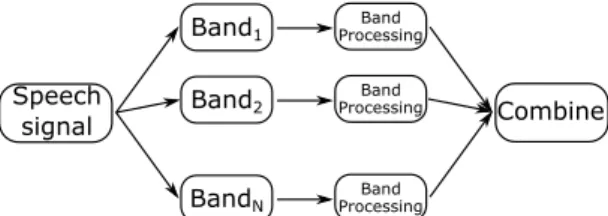
Figure 1:Schematic diagram of multi-band processing
1.1. Multi-band speech recognition
Motivated by psycho-acoustic evidence [16], signal processing considerations [17], and the potential for parallelization, in the multi-band processing paradigm (see Figure 1) the input speech signal is first decomposed into spectral bands, then these bands are processed independently before the information from dif- ferent bands is merged in order to produce the aimed recog- nition result. There are thus three key issues to be addressed in this paradigm, namely the approach used for separating the speech signal into bands, the method of band processing, and lastly, the mechanism used for combining the information ex- tracted from the different bands [18]. In this study, we follow the pipeline described in Kov´acs et al. [19]. Thus we create ten overlapping bands by applying a set of Gabor filters on the mel-scale spectrogram, and then process the resulting features using a Time-Delay Neural Network (TDNN) with a bottleneck consisting of 20 neurons. Lastly, to combine the information re- sulting from the different bands, we trained an additional Deep Rectifier Neural Network (DRNN) using the output from the bottleneck layers as its input.
1.2. Channel dropout
An additional motivation factor for the multi-band paradigm was that of robustness. This was based on the assumption that certain noises that are limited to particular frequency bands would leave unaffected the band processing methods that oper- ate on the other bands. However, when using ANNs as a method of combination, there is a risk that during the process of training the network would learn to overly rely on information originat- ing from particular bands. This means that if a noise heavily affects any of those bands, the final recognition result will also be heavily affected. In an attempt to minimize this risk, we ap- plied channel dropout [20] on the merger network that dropped out entire frequency bands (i.e. all features resulting from the bottleneck layer of the selected band processing networks).
1.3. Related work
One can find many precursors of our work in the speech recog- nition literature. For one, the present study is a deeper ex- ploration of ideas presented in the earlier works of the au- thors [19, 20]. The work reported here is also clearly related to the full combination method of multi-band processing [21]
where a neural network is trained on each combination of bands.
In our case, however, it is not necessary to explicitly train2N (where N is the number of bands used) different networks, as dropout can be also regarded as an ensemble technique [22].
And given that the multi-band approach is a special case of multi-stream processing, the present study is also closely related to the multi-stream framework of Mallidi et al. [23], which is dropping certain streams whilst training the network for band combination. But similarly to the full-combination method, Mallidi et al. trains a large set of deep networks instead of one.
Furthermore, although the dropped streams are replaced by ze- ros in both our work and that of Mallidi et al., the motivation behind this is different (in our case the motivation is the same as it is in dropout [15], in [23] this serves as a way to prepare the merger network for zeros in its input). Lastly, the approach pre- sented here does not rely on explicit performance-monitoring, which means that our solution is simpler to implement, and can evaluate sound files faster than that of Mallidi et al.
2. Methods
In this section we discuss the key methods applied in the present study. First, we briefly describe the approach used to extract the band specific features that constitute the input of the merger network. This is followed by a short discussion of the merger network itself. It should be noted that these discussions are kept intentionally short, as detailed description of these methods are available in the earlier publications of the authors (see [18, 19]) Lastly, we finish the section by a detailed description of the band selection methods applied for choosing the bands to be dropped.
2.1. Processing of individual bands
Here, each individual band was processed in three main stages:
1. Time-frequency processing: we calculated 45-channel log mel-scaled spectrogram using the HTK Toolkit [24], with 160 sample hops, using 400 samples, and applying a 1024- point FFT on the frames.
2. Band formation: to acquire the input spectro-temporal fea- tures for the band processing DNNs, we applied our set of 9 Gabor filters on the input spectrograms. We did so on ten po- sitions of the frequency band, with an overlap of55%. Then we calculated the delta and acceleration coefficients for each feature, and separated the resulting feature vectors into ten equal partitions based on the origin of the features.
3. Bottleneck feature extraction: features for the merger net- works are extracted created from the spectro-temporal fea- tures using TDNs of a specific structure using a 17-frame context with a sub-sampling of 3 frames. Here, the input was first processed by a smaller (200 neurons) layer at 5 po- sitions (using the same weights), which was followed by two fully connected hidden layers applying the rectifier nonlin- earity (each with a 1000 neurons), the second such layer was connected to a linear bottleneck layer (20 neurons), which in turn was connected to the softmax output layer (1997 neu- rons).
2.2. Band combination
The merger network was a DRNN with four hidden layers (each containing a 1000 neurons), and an output layer of 1997 soft- max neurons. The first hidden layer was comprised of ten sub- layers, each taking its input from one band. During the process of training channel dropout was applied on the input of these sub-layers. It should be noted that for the purposes of these experiments, the merger network originally using our in-house neural network implementation was reimplemented in Tensor- flow [25]. In this implementation we also used L2 regulariza- tion (with a scale ofλ = 0.01), and training was carried out using the built-in gradient descent optimizer.
2.3. Band selection for dropout
Band dropout had two important parameters, namely the num- ber of bands than can maximally be dropped out (B = 6), and the probability of dropout activated (P = 0.6). In each batch, we first generated a random probability between 0 and 1, and if this probability was below the P threshold, we generated a sec- ond random number between1andB, and selected the given number of bands to be dropped based on the following policies:
1. Random: each band was chosen with the same probability 2. Weighted: we trained a merging network with an added layer
of 10 weights between the first and second hidden layer, and multiplied the output of each sublayer with the correspond- ing weight. We used the weights at the end of training as probabilities for band selection
3. Leave-1-out: we calculated the probability of a band being dropped based on its impact on the model to attain low error rates. This impact was calculated differently in the three different versions of the policy
(a) We calculated the average increase in error rate in the validation set for each band left out on the models that were trained with no dropout, then divided the results by the sum of the average error increases, so as to get numbers between zero and one that add up to one.
(b) We started to train a model with random dropout, and after each epoch we calculated the probabilities as in the previous version, on the validation set.
(c) We started to train a model with random dropout, and after each epoch we calculated the probabilities as de- scribed in the previous version. However, in this case we did this based on the train set. The justification for this approach was that dropout here was applied in or- der to prevent the model from overfitting on the train set. To achieve this, we were aiming to drop out those bands with the highest probability that the model relied on the most following the last epoch.
3. Experimental data
The proposed methods were evaluated on the Aurora-4 cor- pus [26]. This read speech corpus has two sets for training (both containing 7138 utterances), one consisting of clean speech recorded with a Sennheiser close-talking microphone, and the other consisting of both clean and noise contaminated speech, recorded with the Sennheiser microphone as well as other, sec- ondary microphones. In this study we use exclusively the clean training set, as our initiative was test the noise robustness of our models in the scenario where we do not have any knowledge about the type of noise it would encounter.
Aurora-4 also contains a test-set of 330 utterances, designed to evaluate The trained models. These utterances were recorded in 14 different conditions. For one, they were recorded with the use of the Sennheiser close-talking microphone (Set A) with no additive noise. Six additional sets were created with the same microphone, but in each case having a different real-life addi- tive noise mixed with the speech signal (these, altogether 1980 utterances are referred to as Set B). The same process was re- peated using a set of secondary microphones, resulting in 330 utterances of clean speech (Set C), and 1980 utterances of noise contaminated speech (Set D).
To produce Word Error Rates (WERs) on the Aurora-4 cor- pus, we first used the recipe provided by Kaldi [27] to train a HMM/GMM model. This model was then applied to cre- ate a forced alignment, resulting in 1997 frame-level context- dependent state labels, that we used as targets for neural net- work training. Each neural network was trained on a randomly selected ninety percent of the clean training set, using the frame- level cross-entropy error function. The remaining ten percent of the training set (hereinafter referred to as validation set) was held out for development purposes, and was used for early stop- ping during training. Scoring and decoding was again done with the Kaldi toolkit, the standard tri-gram language model, and the 5k word vocabulary provided with the corpus.
4. Experiments and results
Our experiments on Aurora-4 with the various policies for band selection methods were carried out in two stages. In the first stage we examined the frame-level error rates produced by each model when all bands were available, and when one band was corrupted or missing (e.g. its outputs were replaced by zeros, to emulate the scenario where one band is critically corrupted by noise, or where the bands are processed using different servers, and on is severely delayed or was shut down). Then, in the second stage we evaluated our models on the test set based on the WER scores they produced. Lastly, we compared our results to those reported in the literature.
4.1. Experiments on the validation set
The frame-level results on the validation set are listed in Ta- ble 1. As can be seen in Table 1, there results are very similar.
In fact the only significant difference (atp <0.05) is between the error rates got with random dropout, and those got with con- stant leave-1-out dropout (that is policy (a)). Furthermore, when compared to the error rates got with no dropout, we find that most dropout methods do not increase the error rates, while one method even slightly decreases it. We can also see that the first two leave-one-out policies slightly increased the error rate, but the difference is too small for further deductions.
Table 1:Frame-level error rates on the validation set of Aurora- 4. Reported results are the average of five neural net training.
Dropout selection Error rate
- 27.5%
Random 27.3%
Weighted 27.5%
Leave-1-out (a) 27.7%
Leave-1-out (b) 27.6%
Leave-1-out (c) 27.5%
1 2 3 4 5 6 7 8 9 10
Missing Band 1%
2%
3%
4%
5%
6%
7%
8%
9%
10%
15%
20%
25%
Relative error rate increase
No dropout Random dropout
Figure 2:Comparison of the increase in error rates due to miss- ing bands, in the case of random dropout (solid line) no dropout (dashed line).
Here, we also compare the relative increase of error rates in the case where a band is corrupted. We calculate this increase by first taking the difference between the error rate we got when using all bands, and between the error rate we got when elim- inating one band. Then we divide this result by the error rate got when using all bands. Figure 2 compares the change in er- ror rates when the model is trained with no dropout, and when model is trained with random dropout. As can be seen, our ini- tial prediction – that the band dropout would largely decrease the over-reliance of the model on certain bands – was justified.
Next, we compare the results we got with the random dropout policy with those we got with the weighted policy (where a probability vector for the dropout was created based on the weights of a fully trained model, that had been trained without dropout1 - see Figure 3). As can be seen in Figure 3, the difference between the two curves is minimal. In some cases the performance of one model drops more, and in other cases the opposite is true.
1Here, the (constant) probabilities rounded were as follows:
[0.14,0.13,0.08,0.08,0.12,0.11,0.09,0.08,0.07,0.10]
1 2 3 4 5 6 7 8 9 10
Missing Band 1%
2%
3%
4%
5%
6%
7%
Relative error rate increase
Weighted dropout Random dropout
Figure 3: Comparison of the increase in error rates due to missing bands, in the case of random dropout (solid line) and weighted dropout (dashed line).
1 2 3 4 5 6 7 8 9 10 Missing Band
1%
2%
3%
4%
5%
6%
7%
Relative error rate increase
Random dropout Leave-1-out (a) Leave-1-out (b) Leave-1-out (c)
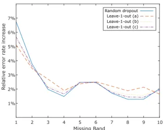
Figure 4:Comparison of the increase in error rates due to miss- ing bands, in the case of random dropout (solid line) and the various leave-1-out strategies ((a) - dashed line, (b) - dotted line, (c) - dotted and dashed line).
Lastly, we make the same comparison with random dropout and leave-1-out dropout (see Figure 4). The results are again mixed. What we can see, however is that policy (a) stands out in the sense that the improvement on the first band is the most pronounced here, but unfortunately it comes at a cost at almost every other band. Policies (b) and (c) are on the other hand very similar. To better interpret the data, we calculated the me- dian and the mean band error rate increase for both. We found that policy (c) performed slightly better both in terms of median (2.01<2.1) and in terms of mean (2.45<2.51). But again the difference was not significant. Because of this, we decided to carry out the word recognition experiments using all three variations of the leave-1-out policy.
4.2. Experiments on the test set
Lastly, we evaluated our select models on the test set of Aurora- 4. The results of these experiments are summarized in Table 2.
We can see in Table 2 a significant divide (accentuated by the horizontal line) between those error scores we got without the use of dropout, and those error scores we got with the use of dropout. What is more is that the difference is significant in all cases (p < 0.00007). However, between the results got with models that had been trained using different dropout selection methods, there is very little difference. Considering our initial results (particularly the similar effect of missing bands on the models trained using various dropout policies) this is not highly unexpected.
Table 2:WERs on the test set of Aurora-4. Results reported are the average of 5 independently trained neural networks.
Dropout selection Word Error Rates (WERs) Set A Set B Set C Set D Total
- 3.1% 17.9% 26.6% 40.2% 27.1%
Random 3.2% 16.0% 23.4% 36.2% 24.3%
Weighted 3.2% 15.9% 24.4% 36.4% 24.4%
Leave-1-out (a) 3.1% 16.0% 24.6% 36.4% 24.4%
Leave-1-out (b) 3.1% 15.9% 24.1% 36.2% 24.3%
Leave-1-out (c) 3.2% 16.0% 24.1% 36.3% 24.3%
Table 3:Comparison of our best result with some recent results given in the literature for the Aurora-4 corpus, using the clean training scenario.
Method WERs
DNN with
26.8%
examples-based enhancement [28]
CNN with channel dropout[20] 26.8%
CNN with data augmentation [29] 25.6%
GMM with
25.5%
auditory spectral enhancement [30]
TDNN with Gabor filters,
25.0%
multi-band processing and channel dropout[19]
Current paper 24.3%
4.3. Comparison to relevant results in the literature Finally, we created a table (see Table 3) that lists the results we found in the recent literature for the same task (i.e. evalu- ation of automatic speech recognition models on the Aurora- 4 test set that had been trained using the clean training sce- nario of the same corpus). As we see in Table 3 while channel dropout (and its data augmentation variant) are already competi- tive, further improvement can be attained when channel dropout is combined with multi-band processing. It should be noted here that the Tensorflow implementation lead to an approximately 3%relative error rate reduction compared to the scores we got earlier using our in-house neural network implementation [19].
This may seem surprising at first, but given that the two methods used a different regularization scheme (as the one we had used earlier was not available in Tensorflow), with different scaling factors (we did not perform exhaustive experiments on the opti- mization of meta-parameters, such as learn-rate, regularization scale, and optimizer used) it is not so unexpected.
5. Conclusions and future work
Here, we investigated various policies to select bands to be dropped out in the process of training in a multi-band speech recognition framework. Our results confirmed that the deploy- ment of earlier introduced channel dropout method [20] in a multi-band environment renders the resulting model more ro- bust against errors in individual frequency bands. The word recognition results then confirmed that this robustness leads to an improved noise robustness on the Aurora-4 corpus. Further- more, we have found that the random selection of bands is al- ready quite competitive.
However, there are still space for improvement in the multi- band framework discussed here. For one, the parameters ap- plied during dropout were also not optimized, but were used on an as-is basis from an earlier study [19]. We also believe that it would be beneficial to investigate whether it is possible to train adversarial networks in a way that for a given speech input its output would be the band numbers that are the most important for recognition given a merger network.
6. References
[1] K.-H. Tan and B. Pang Lim, “The artificial intelligence renais- sance: Deep learning and the road to human-level machine in- telligence,”APSIPA Transactions on Signal and Information Pro- cessing, vol. 7, 07 2018.
[2] W. Xiong, J. Droppo, X. Huang, F. Seide, M. Seltzer, A. Stolcke, D. Yu, and G. Zweig, “Achieving human parity in conversational speech recognition,”CoRR, vol. abs/1610.05256, 2016. [Online].
Available: http://arxiv.org/abs/1610.05256
[3] G. Saon, G. Kurata, T. Sercu, K. Audhkhasi, S. Thomas, D. Dim- itriadis, X. Cui, B. Ramabhadran, M. Picheny, L.-L. Lim, B. Roomi, and P. Hall, “English conversational telephone speech recognition by humans and machines,” inProc. Interspeech 2017, 2017, pp. 132–136.
[4] E. Edwards, W. Salloum, G. Finley, J. Fone, G. Cardiff, M. Miller, and D. Suendermann-Oeft, “Medical speech recognition: Reach- ing parity with humans,” inProc. SPECOM, 2017, pp. 512–524.
[5] K. T. Mengistu and F. Rudzicz, “Comparing humans and au- tomatic speech recognition systems in recognizing dysarthric speech,” inCanadian Conference on AI, ser. Lecture Notes in Computer Science, vol. 6657. Springer, 2011, pp. 291–300.
[6] H. K. Maganti and M. Matassoni, “Auditory processing-based features for improving speech recognition in adverse acoustic con- ditions,”EURASIP J. Audio, Speech and Music Processing, vol.
2014, p. 21, 2014.
[7] B. T. Meyer, “What’s the difference? Comparing humans and ma- chines on the aurora2 speech recognition task,” inProc. Inter- speech 2013, 2013, pp. 2634–2638.
[8] H. Heˇrmansk´y, “Human speech perception: Some lessons from automatic speech recognition,” inProc. TSD 2001, 2001, pp. 187–
196.
[9] O. Scharenborg, “Reaching over the gap: A review of efforts to link human and automatic speech recognition research,”Speech Communication, vol. 49, no. 5, pp. 336–347, 2007.
[10] B. T. Meyer, “Human and automatic speech recognition in the presence of speech-intrinsic variations,” Ph.D. dissertation, Carl- von-Ossietzky University, 2009.
[11] P. R. Adhikari, “Machine vs. human speech recognition,” Helsinki University of Technology, Tech. Rep., 2009.
[12] R. K. Moore,Spoken Language Processing: Where Do We Go from Here? Berlin, Heidelberg: Springer Berlin Heidelberg, 2013, pp. 119–133.
[13] M. Kleinschmidt, “Robust speech recognition based on spectro- temporal processing,” Ph.D. dissertation, Carl-von-Ossietzky Universit¨at, 2002.
[14] P. Duchnowski, “A new structure for Automatic Speech Recogni- tion,” Ph.D. dissertation, MIT, 1993.
[15] G. E. Hinton, N. Srivastava, A. Krizhevsky, I. Sutskever, and R. R. Salakhutdinov, “Improving neural networks by preventing co-adaptation of feature detectors,” CoRR, vol. abs/1207.0580, 2012. [Online]. Available: http://arxiv.org/abs/1207.0580 [16] J. B. Allen, “How do humans process and recognize speech?”
IEEE Trans. Speech and Audio Processing, vol. 2, no. 4, pp. 567–
577, 1994.
[17] S. Rao and W. A. Pearlman, “Analysis of linear prediction, coding, and spectral estimation from subbands,”IEEE Trans. Information Theory, vol. 42, no. 4, pp. 1160–1178, 1996.
[18] G. Kov´acs, “Noise robust automatic speech recognition based on spectro-temporal techniques,” Ph.D. dissertation, University of Szeged, 2018.
[19] G. Kov´acs, L. T´oth, and G. Gosztolya, “Multi-band processing with Gabor filters and Time Delay Neural Nets for noise robust speech recognition,” inIEEE SLT 2018 - Workshop On Spoken Language Technology, 2018, Athens, Greece, December 18-21, 2018, Proceedings, 2018, pp. 242–249.
[20] G. Kov´acs, L. T´oth, D. Van Compernolle, and S. Ganapathy, “In- creasing the robustness of cnn acoustic models using autoregres- sive moving average spectrogram features and channel dropout,”
Pattern Recogn. Lett., vol. 100, no. C, pp. 44–50, Dec. 2017.
[21] A. Hagen, A. Morris, and H. Bourlard, “From multi-band full combination to multi-stream full combination processing in ro- bust asr,” inProc. ISCA Tutorial and Research Workshop ASR, 2000.
[22] K. Hara, D. Saitoh, and H. Shouno, “Analysis of dropout learn- ing regarded as ensemble learning,”CoRR, vol. abs/1706.06859, 2017.
[23] S. H. R. Mallidi and H. Hermansky, “Novel neural network based fusion for multistream ASR,” inProc. ICASSP. IEEE, 2016, pp.
5680–5684.
[24] S. Young, G. Evermann, M. Gales, T. Hain, D. Kershaw, X. A.
Liu, G. Moore, J. Odell, D. Ollason, D. Povey, V. Valtchev, and P. Woodland,The HTK Book (for HTK Version 3.4). Cambridge University Engineering Department, 2006.
[25] M. Abadi, A. Agarwal, P. Barham, E. Brevdo, Z. Chen, C. Citro, G. S. Corrado, A. Davis, J. Dean, M. Devin, S. Ghemawat, I. Goodfellow, A. Harp, G. Irving, M. Isard, Y. Jia, R. Jozefowicz, L. Kaiser, M. Kudlur, J. Levenberg, D. Man´e, R. Monga, S. Moore, D. Murray, C. Olah, M. Schuster, J. Shlens, B. Steiner, I. Sutskever, K. Talwar, P. Tucker, V. Vanhoucke, V. Vasudevan, F. Vi´egas, O. Vinyals, P. Warden, M. Wattenberg, M. Wicke, Y. Yu, and X. Zheng, “TensorFlow: Large-scale machine learning on heterogeneous systems,” 2015, software available from tensorflow.org. [Online]. Available: https://www.tensorflow.org/
[26] H.-G. Hirsch and D. Pearce, “The Aurora experimental frame- work for the performance evaluation of speech recognition systems under noisy conditions,” in Proc. ASR2000-Automatic Speech Recognition: Challenges for the new Millenium ISCA Tu- torial and Research Workshop (ITRW), 2000.
[27] D. Povey, A. Ghoshal, G. Boulianne, L. Burget, O. Glembek, N. Goel, M. Hannemann, P. Motlicek, Y. Qian, P. Schwarz, J. Silovsky, G. Stemmer, and K. Vesely, “The kaldi speech recog- nition toolkit,” inProc. ASRU, 2011.
[28] D. Baby, J. F. Gemmeke, T. Virtanen, and H. V. hamme,
“Exemplar-based speech enhancement for Deep Neural Network based automatic speech recognition,” inProc. ICASSP, 2015, pp.
4485–4489.
[29] L. T´oth, G. Kov´acs, and D. V. Compernolle, “A perceptually in- spired data augmentation method for noise robust CNN acoustic models,” inSpeech and Computer - 20th International Confer- ence, SPECOM 2018, Leipzig, Germany, September 18-22, 2018, Proceedings, 2018, pp. 697–706.
[30] M. J. Alam, P. Kenny, , and D. OShaughnessy, “Robust feature extraction based on an asymmetric level-dependent auditory fil- terbank and a subband spectrum enhancement technique,”Digital Signal Processing, vol. 29, pp. 147–157, 2014.