Working Paper 2018:19
Department of Economics
School of Economics and Management
Organizing Time Banks: Lessons from Matching Markets
Tommy Andersson Ágnes Csehz
Lars Ehlers Albin Erlanson
July 2018
Revised: March 2019
Organizing Time Banks:
Lessons from Matching Markets
∗Tommy Andersson†, Ágnes Cseh‡, Lars Ehlers§, and Albin Erlanson¶ First version: October, 2014. This version: March 6, 2019.
Abstract
A time bank is a group of people that set up a common platform to trade services among them- selves. There are several well-known problems associated with time banks, e.g., high overhead costs and difficulties to identify feasible trades. This paper constructs a non-manipulable mech- anism that selects an individually rational and time-balanced allocation which maximizes ex- changes among the members of the time bank (and those allocations are efficient). The mechanism works on a domain of preferences where agents classify services as unacceptable and acceptable (and for those services agents have specific upper quotas representing their maximum needs).
Keywords: market design; time banking; priority mechanism; non-manipulability.
JEL Classification: D82; D47.
1 Introduction
Time banks have now been established in at least 34 countries. In the United Kingdom, for example, there are more than 300 time banks, and time banks are operating in at least 40 states in the United States (Cahn, 2011).1 A time bank is a group of individuals and/or organizations in a local community that set up a common platform to trade services among themselves. Members of a time bank earn time credit for each time unit they supply to members of the bank and the earned credit can be spent to receive services from other members of the bank. Very few time banks are not based on a “one-for- one” time system, meaning that members of the time bank need not get one unit of time back for each unit of time they supply (see also Footnote 7 or Croall, 1997). Therefore, we consider the most commonly used “one-for-one” time banks. For example, a gardener who supplies two hours of time
∗We are grateful to four anonymous referees, Michael Ostrovsky (coeditor), Peter Biró, Jens Gudmundsson and Flip Klijn for many useful and constructive comments. All authors gratefully acknowledge financial support from the Jan Wallander and Tom Hedelius Foundation. Andersson is also grateful to Ragnar Söderbergs Stiftelse (E8/13) for financial support. Cseh was supported by the Hungarian Academy of Sciences (KEP-6/2017), its Momentum Programme (LP2016- 3/2016) and its János Bolyai Research Fellowship. Ehlers is grateful to the SSHRC (Canada) and the FRQSC (Québec) for financial support.
†Lund University, Department of Economics. E-mail:tommy.andersson@nek.lu.se.
‡Hungarian Academy of Sciences, Institute of Economics. E-mail:cseh.agnes@krtk.mta.hu.
§Université de Montréal, Département de Sciences Économiques. E-mail:lars.ehlers@umontreal.ca.
¶Stockholm School of Economics, Department of Economics. E-mail:albin.erlanson@hhs.se.
1A more thorough description of timebanking and time banks will be provided in Section 2.
may, for example, receive two hours of child care in return for his gardening services. Ozanne (2010) reported that the most commonly exchanged services included gardening, giving lifts, befriending, do-it-yourself jobs, dog walking, and computer training. Even if time banks traditionally have had a very simple organization, most of the nowadays existing time banks take advantage of computer databases for record keeping and a broker (physical coordinator) that keeps track of transactions and match requests for services with those who can provide them (Seyfang, 2003, 2004; Williams, 2004).
A critical factor for a time bank to function smoothly is the coordination device that matches re- quests for services with those who can provide them. Our basic observation is that this type of service exchange shares many features with some classical markets previously considered in the matching literature, including, e.g., housing markets (Scarf and Shapley, 1974; Abdulkadiro˘glu and Sönmez, 1999; Aziz, 2016b), organ markets (Roth et al., 2004; Biró et al., 2009; Ergin et al., 2017), one-to-one matching problems (Gale and Shapley, 1962), and markets for school seats (Abdulkadiro˘glu and Sön- mez, 2003; Kesten and Ünver, 2015). In particular, if a time bank is organized as a matching market, the time bank will have a structure of what in the matching literature is known as a many-to-many matching market. This follows since any member of a time bank can trade services with any other member of the very same time bank and there are no obstacles that prevent a member of a time bank to supply and receive multiple services from members of the very same time bank. Such matching markets have previously been considered by, e.g., Echenique and Oviedo (2006), Konishi and Ünver (2006), and Hatfield and Kominers (2016).
The above mentioned classical matching markets are centralized as the agents in the system (e.g., tenants, patients, or students) report their preferences over the items to be allocated (e.g., houses, organs, or school seats) to a clearing house and a mechanical procedure (or mechanism) determines the final allocation based on the reported preferences and a set of predetermined axioms. As will be described in more detail in Section 2, even if time banks often take advantage of computer databases, there is no mechanical procedure that determines the trade of services among the members in the bank based on reported preferences, and it is exactly in this respect that time banks can learn from insights in classical matching markets.
By organizing a time bank as a matching market, it is possible to solve a number of problems which have been associated with time banks. For example, time banks typically encounter long run organizational sustainability problems since they experience high overhead costs, e.g., as staff is needed to keep the organization running and, in particular, to help out in the coordination process (Seyfang, 2004). Moreover, independently of if possible exchanges are identified manually by a bro- ker or if members propose exchanges through an internet-based software, it is challenging to identify and coordinate longer trading cycles.2 Time bank members sometimes experience that time credits are comparatively easy to earn but harder to spend (Ozanne, 2010), i.e., the reverse situation compared to conventional money which generally is hard to earn, but easy to spend. The consequence of the latter problem is that potential members never join time banks simply because there is a risk that they provide more time than they get back.
A computer-based clearing house, e.g., an internet-based interface for reporting needs and requests together with an algorithm for matching needs and requests, on the other hand, can help in reducing
2In fact, some members have experienced difficulties to understand the mechanism for making trades (Ozanne, 2010;
Seyfang, 2004) and, consequently, the role of the broker is important even when an internet-based software is used.
costs related to coordination. Such an algorithm can also identify and coordinate longer trading cycles which in turn will lead to a maximal number of exchanged time units and, consequently, to an efficient outcome. In addition, problems related to participation concerns can be solved by restricting the algorithm to only propose individually rational time-balanced exchanges, i.e., exchanges where all members of the bank only receive services they have requested and get exactly as much time back as they supply to the bank.
The above discussions and observations also motivate the interest in (time) allocations that are individually rational, maximal, and time-balanced. A first observation is that such allocations always exist on the general preference domain. This follows since the allocation in which all agents receive their initial time endowments is individually rational and satisfies time-balance. The conclusion then follows directly from the observation that the number of individually rational allocations that satisfy time-balance is finite and, consequently, that there exists an allocation among those which maximizes trade in the time bank.
However, even if an allocation satisfying these specific properties can be identified, two new problems arise. First, it is often natural to require that the algorithm should be designed in such fashion that it is in the best interest for all agents to report their preferences truthfully (non-manipulability).
This property is incompatible with individual rationality, efficiency and time-balance on a general preference domain (Sönmez, 1999, Corollary 1).3 Second, because members of a time bank can exchange multiple time units, it is not clear that it is easy for members to generally rank any two
“consumption bundles”. For example, is two hours of hairdressing, two hours of gardening and one hour of babysitting strictly better, equally good, or less preferred to one hour of hairdressing, one hour of gardening and three hours of housekeeping? Hence, it may be an obstacle for members to report their preferences if multiple time units are on stake and if multiple agents are allowed to be involved in a longer trade.
We show that if agents’ preferences satisfy certain conditions, the above two problems are no longer present. In some settings, the considered preference domain is clearly unrealistic (e.g., in the school choice problem by Abdulkadiro˘glu and Sönmez, 2003). In the case of timebanking, however, they provide a reasonable approximation as will be explained below. The considered restricted domain is an extension of the dichotomous domain popularized by Bogomolnaia and Moulin (2004).4 In the considered domain, individual preferences are completely described by (i) partitioning the members of the bank (or, equivalently, the services that the members provide) into two disjoint subsets con- taining acceptable and unacceptable members, and by (ii) specifying a member specific upper time bound for each acceptable member. The former condition reflects that an agent is not necessarily interested in all services provided in the bank (an agent’s “horizontal” preference) whereas the latter condition captures the idea that an agent may, for example, be interested in at most one haircut but can accept up to 10 hours of babysitting (an agent’s “vertical” preference). One advantage of adopting this preference domain is that it facilitates for agents to report their preferences as they just need to report all unacceptable members and all acceptable members with their upper bounds in contrast to
3This impossibility should come as no surprise given the results in, e.g., Hurwicz (1972), Green and Laffont (1979), Roth (1982), Alcalde and Barberà (1994), Barberà and Jackson (1995), or Schummer (1999).
4In fact, Bogomolnaia and Moulin (2004) and a series of subsequent papers, argue that it is natural to consider a dichoto- mous domain in problems involving “time sharing”.
reporting a ranking over all possible bundles.5 Agents then strictly prefer receiving more time units from acceptable services to receiving fewer time units from acceptable services (without exceeding upper bounds or receiving unacceptable services). In this sense, an agent may have many different indifference classes and preferences are dichotomous over single services and polychotomous over bundles of services.
We define and apply a priority mechanism to solve the problem of exchanging time units between members in a time bank. It is demonstrated that the priority mechanism can be formulated as a min- cost flow problem (Proposition 1). Consequently, it is not only possible to identify time-balanced trades, it is also computationally feasible. The definition of the priority mechanism is flexible as it can be adopted on the restricted preference domain or the general domain. Our main result shows that the priority mechanism is non-manipulable on the restricted preference domain and that it always makes a selection from the set of individually rational, maximal, and time-balanced allocations (The- orem 1). To prove this result, a number of novel graph theoretical techniques are needed. In particular, Appendix B demonstrates an equivalence result between the min-cost flow problem and a circulation- based maximization problem.6 Using graph theoretical tools and in particular min-cost/max-weight formulations to solve matching problems is common in the literature. In the house allocation problem with dichoutomous preferences Aziz (2016b) formalizes a bipartite graph and solves for a max-weight matching. His graph construction is based on having houses on one side and agents on the other side.
This is in contrast to our approach where we make copies of agents. Furthermore, our graph construc- tion and the solution is more intricate since agents’ can have more than one object. Because finding a maximal alloaction is more involved in our problem and a potential manipulation is more complex we use the graph theoretical tools in proving non-manipulability of the mechanism. This is not needed in Aziz (2016b) because of the less complex optimization problem.
A variety of real-life problems have previously been considered in the matching literature in- cluding the above mentioned house allocation problem, kidney exchange problem and school choice problem. There are, however, several differences between these problems and the time banking prob- lem. For example, in the time banking problem, an agent may receive and supply multiple time units.
In the school choice problem and the kidney exchange problem, on the other hand, students are allo- cated at most one school seat and a patient is involved in at most one kidney exchange, respectively.
Furthermore, in many matching problems including, e.g., the school choice problem and the house allocation problem, agents’ (reported) preferences are typically strict and indifference relations are consequently not allowed (while the kidney exchange problem is often defined on a dichotomous domain). Generalizations to allow for a weak preference structure have recently been proposed by Alcalde-Unzu and Molis (2011) and Jaramillo and Manjunath (2012). However, both these papers only allow agents to trade at most one object.
The papers closest to the model investigated in this paper are Athanassoglou and Sethuraman (2011), Aziz (2016a), Biró et al. (2017) and Manjunath and Westkamp (2018), which we describe below.
5The strict preference domain is often considered in the matching literature. However, the dichotomous domain is much smaller in size than the strict preference domain, but is not a subset of the strict domain since indifference relations are allowed in the former but not in the latter domain.
6The min-cost flow problem is considered in the main part of the paper since it is more intuitive and, moreover, can be introduced using minimal notation.
Athanassoglou and Sethuraman (2011) and Aziz (2016a) consider a housing market where ini- tial endowments as well as allocations are described by a vector of fractions of the houses in the economy. The fractional setting makes it possible to analyze, e.g., efficiency based on (first-order) stochastic dominance, and it is demonstrated that the efficiency and fairness notions of interest con- flict with non-manipulability. Even if a similar impossibility is present in the model considered in this paper, the fractional setting is analyzed using different axioms and mechanisms. In addition, Athanas- soglou and Sethuraman (2011) and Aziz (2016a) are unable to find any positive results related to non-manipulability in their considered reduced preference domains.
Biró et al. (2017) consider, as this paper, a model where agents are endowed with multiple units of an indivisible and agent-specific good, and search for balanced allocations. In their reduced preference domain, agents have responsive preferences over consumption bundles. On this reduced domain, they demonstrate that, for general capacity configurations, no mechanism satisfies individual rationality, efficiency, and non-manipulability. Given this negative finding, they characterize the capacity con- figurations for which individual rationality, efficiency and non-manipulability are compatible. They also demonstrate that for these capacity configurations, their defined Circulation Top Trading Cycle Mechanism is the unique mechanism that satisfies all three properties of interest. Hence, the main dif- ference between this paper and Biró et al. (2017) is that they consider a different preference domain and, consequently, need a different mechanism to escape the impossibility result.
Manjunath and Westkamp (2018) have independently considered a model closely related to the one considered here. In their model, an agent can supply distinct services but at most one time unit of each service (recall that agents in our model supply one service but, possibly, several time units of it).
They also require time-balance and consider a preference domain classifying services as unacceptable and acceptable (there is no need to specify upper bounds on services since each service is available in one unit). Given this, Manjunath and Westkamp (2018) define a priority mechanism over the set of individually rational and efficient allocations. The main differences between their work and ours is that (i) they allow agents having distinct services whereas each agent in our model has a specific service that comes in multiple copies, (ii) their priority mechanism chooses from the set of individu- ally rational and efficient allocations whereas ours chooses from the set of individually rational and maximal allocations (and as we show in Example 3, any priority mechanism may choose different allocations in their setting and in ours), and (iii) for the non-manipulability result they use a bipartite graph approach whereby capacities for unacceptable services are reduced one-by-one (following the priority order) whereas we use a direct circulation based graph with upper capacities on edges (where the min-cost flow corresponds to the allocation chosen by the priority mechanism).
The remaining part of the paper is outlined as follows. Section 2 gives a more detailed introduction to timebanking and provides some descriptive statistics of the time banks associated withTimeBanks USA. Section 3 introduces the theoretical framework and some basic definitions. The priority mech- anism is presented in Section 4. The main results are presented in Section 5. Section 6 discusses the main findings of the paper and some extensions of the considered timebanking model. Section 7 concludes the paper. All proofs are relegated to the Appendix.
2 Timebanking
As already explained in the Introduction, a time bank is a group of individuals and/or organizations in a local community that set up a common platform to trade services among themselves. This section gives a more detailed description of the fundamental ideas underlying time banks and how time banks attempt to integrate in a larger society. This section also provides some details ofTimeBanks USA(the largest time bank operating in the United States).
2.1 Time Banks and the Society
Even if concepts closely related to timebanking dates back to the 19th century, timebanking was popularized and pioneered in the 1990s by Edgar Cahn and Martin Simon in the United States and the United Kingdom, respectively. One of the fundamental ideas in timebanking is that one hour of service generates one time credit regardless of the provider or the nature of the service performed.
This rule is deeply rooted in the philosophical view that even if services are valued differently, human beings share fundamental equality.7
Because time bank members exchange services among themselves in local communities, potential positive external welfare effects of timebanking includes resilient local communities, extended social networks and informal neighbourhood support (this is also part of the core values of timebanking, see footnote 7). Even if there is limited research on timebanking, there exists empirical evidence that time banks indeed help in building strong local networks. For example, in a UK based case study, Boyle et al. (2006) showed that time banks not only help their members to extend their social networks but also that time banks are an effective way of developing reciprocal relationships between members in the bank. In another UK based case study, Seyfang and Smith (2002) demonstrated that time banks are successful in attracting participants both from socially excluded groups (people on benefit programs, from low income households, etc.) and from groups that normally not are involved in traditional volunteering. For example, 16 percent of traditional volunteers have an annual income below£10,000 but the corresponding number for the time bank members in their survey was 58 percent. Furthermore, 40 percent of traditional volunteers are not in formal employment compared to 72 percent of the time bank members.
The above findings show that a majority of the time bank members belong to socially excluded groups and low income communities are also supported in other studies in both the United Kingdom (Seyfang, 2003) and the United States (Collom, 2007).8 This could explain the existence of time banks in a world where monetary transfers are available. Namely, because most members have small social networks and in many cases also lack both income and employment, timebanking is one way to be included in a social network and to increase welfare. Collom (2007) also finds that the single most important reason for joining a time bank is to expand purchasing power through an alternative
7The philosophy of timebanking rests on five core values: assets, redefining work, reciprocity, social networks, and respect. The idea that one hour of service always generates one time credit, the so-called one-for-one time system, is embedded in these core values, see Cahn (2000). It should also be noted that a small minority of all time banks are not based on a one-for-one time system, meaning that members of the time bank need not get one unit of time in return for each unit of time they supply (Croall, 1997). This paper, however, restricts attention to one-for-one time systems.
8Most of the studies in the literature, consequently, focuses focus on socially excluded and low income groups. An exception is Ozanne (2010) where it is demonstrated that time banks has provided high benefits in the form of social, human, physical and cultural capital also within affluent groups.
currency. Seyfang (2003) found that persons also join time banks, e.g., to meet other participants, to help other members and to get more involved in the local neighbourhood. Similar motives are recoded by Collom (2007) and Caldwell (2000). Joining a time bank may also have other positive spill-overs.
For example, when the concept of time banking was used within health care provisions, it was found that there were tangible benefits, both practical and motivational, to health services users (Boyle and Bird, 2014; Simon, 2003).
2.2 Organization and Descriptive Statistics
In most time banks, a broker is employed to manage the bank, maintain the database, record transac- tions, recruit new members, etc. (Seyfang, 2004; Williams, 2004). A “matching mechanism” helps the broker to coordinate requests for services with those who can provide them. In some time banks, this mechanism is simple and the broker manually matches requests with offers (Seyfang, 2003). The obvious drawback for such a mechanism is the difficulty to identity and coordinate longer trading cy- cles. Hence, this type of matching device naturally restricts trade to bilateral exchanges. A few large time banks, e.g.,TimeBanks USAandTimebanking UK, have developed their own computer software where members can see what other members offer and keep track of their own activity. As will be de- scribed below, the members themselves then make requests and offers through the computer software.
Also in this case, however, it is difficult to coordinate longer trading cycles as members only can see their own activity.
An example of computer software for timebanking is Community Weaver 3 which is the most recent software launched byTimeBanks USA. This software allows members to register their talents in 11 different categories including, e.g., education, transportation, business services, recreation, and companionship.9 Each of these categories also have subcategories. The category “education”, for example, contains, e.g., the subcategories advocacy, computers, languages, finances, and tutoring.
When a member have registered her talents, she can formally offer her services and start making requests. An offer is essentially a registration on the online platform that enables other members to see and request her talents. If a member approves a request, she receives the agreed amount of time credits and the member that receives the service is credited by the same amount of time credits. The software also keeps track of the time credit balance for each member.
Even if the first time banks saw the light of the day in the 1990s, it took another 20 years before the concept of timebanking had a serious impact in society. Dash and Sandhu (2018) report that the first time bank in the United Kingdom was set up in 1996 but that only 2,200 persons had joined a time bank in 2003. Eight years later after additional experimentation, learning, and expansion, there were around 30,000 registered members in the United Kingdom, 30,000 registered members in the United States and an additional 100,000 members scattered across 34 countries (Cahn, 2011). This number has continued to grow. In 2014, there were around 35,000 members in the United Kingdom and even more in the United States.10
To the best of our knowledge, there exists no public database that provides detailed informa- tion about time banks worldwide. Instead, this section will end with some descriptive statistics of TimeBanks USA(the largest time bank operating in the United States). This bank currently has 107
9All data and documentation related toTimeBanks USAstated in this section is available in the Online Appendix.
10These figures are from Boyle and Bird (2014) andwww.timebanks.org(retrieved 2019–02–05).
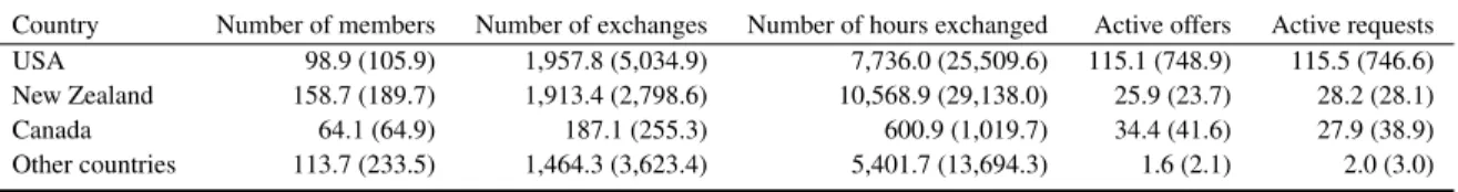
branches in the United States spread out over 33 states, and it also operates in Australia, Canada, France, Greece, Guatemala, Israel, New Zealand, South Africa, South Korea, and United Kingdom (see Table 1). Even if not all registered branches are active, Table 2 provides some more detailed in- formation about the active branches. As can be seen from the table, a time bank located in the United States have on average around 100 members and have on average performed 1,958 trades since April 2015. These trades involved on average 7,736 time units meaning that each time exchange was on average for 3.95 hours. As also can be seen from Table 2, the average time bank in the United States had 115.1 registered active offers and 115.5 active requests on January 15, 2019. The US figures from Table 2, therefore, roughly translates to that each member, in an active branch, on average had one active offer and one active request on January 15, 2019.
Table 1:Descriptive data ofTimeBanks USA.
Country Number of branches Active branches Represented in states/provinces/regions
USA 107 84 33 out of 50
New Zealand 30 28 7 out of 16
Canada 11 9 5 out of 10
Other countries 8 7 –
∗The data was collected fromwww.timebanks.orgon 2019–01–15 and it is available in the Online Appendix.
Table 2:Mean summary statistics for the active time banks in Table 1.
Country Number of members Number of exchanges Number of hours exchanged Active offers Active requests
USA 98.9 (105.9) 1,957.8 (5,034.9) 7,736.0 (25,509.6) 115.1 (748.9) 115.5 (746.6)
New Zealand 158.7 (189.7) 1,913.4 (2,798.6) 10,568.9 (29,138.0) 25.9 (23.7) 28.2 (28.1)
Canada 64.1 (64.9) 187.1 (255.3) 600.9 (1,019.7) 34.4 (41.6) 27.9 (38.9)
Other countries 113.7 (233.5) 1,464.3 (3,623.4) 5,401.7 (13,694.3) 1.6 (2.1) 2.0 (3.0)
∗All values are mean values (standard deviation within brackets).
3 The Model and Basic Definitions
This section introduces the time banking problem together with some definitions and axioms.
3.1 Agents, Bundles, and Allocations
LetN ={1, . . . , n}denote the finite set of agents. Each agenti∈N is endowed withti ∈Nunits of time which can be used to exchange services with agents inN. Lett= (t1, . . . , tn)denote the vector of time endowments. Because the exact nature of the services is of secondary interest, the problem will be described in terms of the time that an agent receives from and provides to other agents in N. Letxij denote the time that agenti ∈ N receives from agent j ∈ N, or, equivalently, the time that agentj provides to agent i. Here, xii represents the time that agent i ∈ N receives from or, equivalently, spends with himself. It is assumed thatxijbelongs to the setN0of non-negative integers (including 0) representing standardized time units (e.g., 0 minutes for zero units, 30 minutes for one unit, 60 minutes for two units, etc.)
The time that agent i ∈ N receives from the agents in N can be described by the bundle (or vector)xi = (xi1, . . . , xin). The bundle where agenti∈ N spends all time with himself is denoted
byωi (whereωii = ti andωij = 0forj 6= i). An allocationx = (x1, . . . , xn)is a collection ofn bundles (one for each agent inN). An allocation isfeasibleif
n
X
j=1
xij = tifor alli∈N , (1)
n
X
j=1
xji = tifor alli∈N . (2)
This means any agentireceives the same amount of time from other agents that the agent supplies to other agents (recall that an agent can receive time from and spend time with himself). In this sense, any feasible allocation satisfies the time-balance conditions (1) and (2). In the remaining part of the paper, it is understood that any allocation is feasible.
3.2 Preferences and Preference Domains
A preference relation for agenti ∈ N is a complete and transitive binary relationRi over feasible bundles such that xiRix0i whenever agent ifinds bundle xi at least as good as bundle x0i. LetPi andIi denote the strict and the indifference part of Ri, respectively. Let Ri denote the set of all preference relations of agent i ∈ N. A (preference) profile R is a list of individual preferences R = (R1, . . . , Rn). The general domain of profiles is denoted byR = R1× · · · × Rn. A profile R ∈ R may also be written as (Ri, R−i) when the preference relation Ri of agent i ∈ N is of particular importance.
A restricted preference domain R˜ = ˜R1 × · · · × R˜n ⊂ R will be considered for our main results. As explained in the Introduction, this restricted domain is based on the idea that any preference relationRi ∈R˜i:
(a) partitions the set of agentsN\{i}into two disjoint sets containing acceptable and unacceptable agents, denoted byAi(Ri)⊆N \ {i}andUi(Ri) =N\(Ai(Ri)∪ {i}), respectively, and;
(b) associates with each acceptable agentj ∈Ai(Ri)an upper bound¯tij ∈N0 on how much time agentiat most would like to receive from agentj.
Here, one may interpret (a) as agenti’s “horizontal preference” over acceptable and unacceptable services and (b) as agenti’s “vertical preference” of how much agentineeds at most of each service.
Then, for agenti∈N, the preference relationRi belongs toR˜iif for any allocationsxandy:
(i) ωiPixiifxik >0for somek∈Ui(Ri)orxij >t¯ij for somej∈Ai(Ri), (ii) xiIiyiif bothωiPixiandωiPiyi,
(iii) yiPixi ifyiRiωi,xiRiωiandP
j∈Ai(Ri)yij >P
j∈Ai(Ri)xij, or (iv) yiIixiifyiRiωi,xiRiωiandP
j∈Ai(Ri)yij =P
j∈Ai(Ri)xij.
The first condition states that an agent strictly prefers not to be involved in any trade rather than re- ceiving time from an unacceptable agent or exceeding his upper bound from an acceptable agent. The
second condition means that an agent is indifferent between any two bundles containing an unaccept- able agent or exceeding his upper bound from an acceptable agent. The last two conditions reflect a monotonicity property and state that an agent weakly prefers bundles with weakly more acceptable agents whenever bundles do not contain any unacceptable agents and as long as the time bounds¯tij are not exceeded for acceptable agents.
In the Introduction we motivate the preference domain further. Our assumptions captures certain aspects of existing time banks, such as that you can classify your services supplied in various cate- gories and then the other agents can request a certain services. There are clearly other assumptions on preferences that one can make, and eventually it is a matter of whether a particular application fits to the model or not. In Section 7 we also discuss two other applications different from the timebanking one. One being shift-exchange among workers, for instance at a hospital, and the second is seminar exchange for PhD students.
Remark 1. For the restricted domainR, a report˜ Ri for agenti∈N is given by a set of acceptable agentsAi(Ri)together with an upper time bound¯tij for eachj∈Ai(Ri). An equivalent formulation of the reported preference for agenti∈N is a vector¯ti = (¯ti1, . . . ,¯tin) ∈Nn0 wheret¯ii =ti. Then
¯tij = 0stands forj ∈ Ui(Ri), i.e., agentiis willing to accept at most zero time units from agentj.
Whether the first or the second formulation is used is just a matter of choice.
Remark 2. For any agenti∈N andRi ∈R˜i, the preferenceRiis dichotomous over single services because they are partitioned into acceptable services and unacceptable services. The preferenceRiis polychotomous over bundles of services in the following way: for anyh= 0,1, . . . ,min{ti,P
j∈Ai(Ri)¯tij}= m, all allocationsx andysuch that for allj ∈ Ai(Ri) xij ≤ t¯ij andyij ≤ ¯tij for allj ∈ Ai(Ri),
xik = 0 =yikfor allk∈Ui(Ri)andP
j∈Ai(Ri)yij =h=P
j∈Ai(Ri)xij are ranked indifferent by Ri. LetI(h)denote this indifference class. Then underRi all allocations inI(m)are strictly pre- ferred to all allocations inI(m−1), and in general, forh= 1, . . . , m, underRiall allocations inI(h) are strictly preferred to all allocations inI(h−1). Thus,Ricontainsm+2indifference classes (where I(0) ={ωi}andωi is strictly preferred to all allocations which are positive for some unacceptable service or exceeds the time bound for an acceptable service). In this sense, preferences belonging to R˜i are polychotomous over bundles of services (where the upper bounds are incorporated) and at the
same time dichotomous over single services.
3.3 Axioms and Mechanisms
Let F(R) denote the set of all feasible allocations at profile R ∈ R˜. Allocation x ∈ F(R) is individually rationalif, for alli∈N,xiRiωi. Allocationx∈ F(R)Pareto dominatesallocationx0 ∈ F(R)ifxiRix0ifor alli∈N andxjPjx0jfor somej∈N. An allocation isefficientif it is not Pareto dominated by any feasible allocation. An allocation x ismaximal atR if P
i∈N
P
j∈Ai(Ri)xij ≥ P
i∈N
P
j∈Ai(Ri)x0ij for all individually rational allocationsx0. All individually rational and maximal allocations at profileR∈R˜are gathered in the setX(R)⊂ F(R). Note thatX(R)6=∅for allR∈R˜ and that anyx∈ X(R)is efficient.11
11Ifxis not efficient, then there exists an individually rational allocationx0such thatx0iRixifor alli∈Nandx0jPjxj
for somej∈N. But thenP
i∈N
P
j∈Ai(Ri)xij<P
i∈N
P
j∈Ai(Ri)x0ijmeaning thatxis not maximal, a contradiction.
A mechanism ϕwith domain R˜ chooses for any profile R ∈ R˜ a feasible allocation ϕ(R) ∈ F(R). Mechanismϕis manipulable at profileR ∈R˜ by an agenti∈N if there existsR0isuch that R0 = (R0i, R−i) ∈ R, and for˜ x = ϕ(R) andx0 = ϕ(R0)we havex0iPixi. If mechanismϕis not manipulable by any agenti∈N at any profileR∈R, then˜ ϕisnon-manipulable(on the domainR).˜ 4 Priority Mechanisms
Often in real life, the chosen allocation is based on a priority mechanism: any such mechanism uses a priority-ordering, which may be deduced from a lottery or from a schematic update based on previous allocation rounds. Letπ : N 7→ N be an exogenously given priority-ordering where the highest ranked agent isi∈N withπ(i) = 1, the second highest ranked agent isi0 ∈N withπ(i0) = 2, and so on.
GivenR∈R,˜ i∈N andZ∗ ⊆ X(R), allocationx∈ Z∗belongs to the setXi,Z∗(R)ifxiRix0i for allx0 ∈ Z∗, i.e., if allocationxis weakly preferred to any allocation in the setZ∗under preference Ri. In the special case where the setZ∗is based on the choice made by some agenti0 6=ifor some profileR∈R, i.e., where˜ Z∗ =Xi0,Z∗∗(R)for someZ∗∗ ⊆ X(R), the setXi,Z∗(R)is denoted by Xi,i0(R).
Definition 1. An allocationx∈ X(R)is agent-i-optimal at profileR∈R˜ifx∈ Xi,X(R)(R).
Note the difference between the setsXi,X(R)(R)andXi,Z∗(R). The former set contains all agenti’s most preferred allocations in the setX(R)whereas the latter set contains all agenti’s most preferred allocations in a subsetZ∗ofX(R).
Definition 2. Let π be a priority ordering and N = {i1, . . . , in} be such that π(ik) = k for all k= 1, . . . , n. Thenx∈ X(R)is aπ-priority allocation at profileR∈R˜ if:
(i) xbelongs toXi1,X(R)(R),
(ii) xbelongs toXik,ik−1(R)for allk= 2, . . . , n.
One way to think about the set of priority allocations is the following. First, the highest ranked agent identifies all his most preferred allocations in the setX(R). Then the agent with the second highest priority identifies all his most preferred allocations in the set identified by the highest ranked agent, then the agent with the third highest priority identifies all his most preferred allocations in the set identified by the second highest ranked agent, and so on. Formally, this means that ifxis aπ-priority allocation, then:
x∈ Xin,in−1(R)⊆ Xin−1,in−2(R)⊆. . .⊆ Xi2,i1(R)⊆ Xi1,X(R)(R)⊆ X(R). (3) Note that a priority allocation is agent-i-optimal for the agent i ∈ N withπ(i) = 1. Moreover, all agents inN are, by construction, indifferent between all allocations in the setXin,in−1(R).
Definition 3. A mechanismϕis a priority mechanism if there exists a priority orderingπ such that for all profilesR∈R˜ the mechanismϕselects aπ-priority allocation from the setX(R).
Since a priority mechanism always makes a selection from the setX(R), it chooses an individually rational, maximal, and time-balanced allocation (which is efficient).
5 Results
As we show in Section 6, it is impossible to construct an individually rational, efficient, and non- manipulable mechanism on the general domainR. Our first main result demonstrates that this impos- sibility can be avoided on the restricted domainR˜if trades are based on a priority mechanism.
Theorem 1. Any priority mechanism with domainR˜ is non-manipulable.
In most settings proving non-manipulability of a priority mechanism is rather straight forward, e.g., Svensson (1994). In our setting with multiple objects and potentially different number of objects the scope for manipulation is much larger. The maximal set of allocations changes in a complex manner if one agent reports something slightly different. To prove non-manipulability we formulate a circulation flow network corresponding to the allocation in the priority mechanism. This enables us to keep track of changes from potential manipulations using the network formulation. The proof boils down to showing that no agent can ever gain by reducing the number of desired copies from an acceptable agent. For details of the argument and the construction of the network see Appendix B.
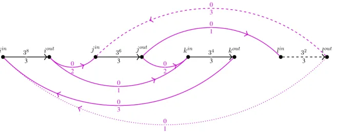
In Proposition 1 below, it is demonstrated that a priority mechanism can be formulated as a min- cost flow problem. To formulate this problem, a bipartite graph needs to be defined and specific values must be attached to the vertices and the edges in the graph.
Definition 4. For any profileR∈R, the bipartite graph˜ g= (N, M, E, u)is defined by two disjoint sets of vertices,N andM, a set of edges,E, and a profile of upper boundsu= (u(i, l))(i,l)∈E on the flow between any two edges, defined by:
(i) N ={1, . . . , n},
(ii) M ={n+ 1, n+ 2, . . . , n+n},
(iii) E ={(i, n+j)∈N×M :j∈Ai(Ri)orj=i}, and
(iv) for alli ∈ N and each edge(i, n+j) ∈ E wherej ∈ Ai(Ri)we setu(i, n+j) = ¯tij and u(i, n+i) =ti.
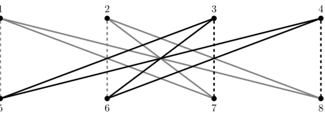
Example 1. Let N = {1,2,3,4}, t1 = t2 = 1 and t3 = t4 = 2. Let R ∈ R˜ be such that A1(R1) = A2(R2) = {3,4}(with¯t13 = ¯t14 = ¯t23 = ¯t24 = 1) andA3(R3) = A4(R4) = {1,2}
(with¯t31= ¯t32= ¯t41= ¯t42= 2). The constructed graphgis depicted in Figure 1.
The interpretation of the graphgis that the agents inM should be regarded as copies of the agents inN and in particular, agentn+i ∈ M is the copy of agenti ∈ N. Furthermore, agentsi ∈ N andn+j ∈ M are connected by an edge if agentjis acceptable for agentior ifj = i. Because an allocation will be defined by the flows between the agents inN andM, the above construction guarantees thatn+j∈Mcan only provide time for an agenti∈N if agentifinds agentjacceptable or if agentj is his own copy. Finally, the upper bound on flow fromn+jtoiwherej ∈Ai(Ri)is equal to the upper bound of how much time agentiwants from agentj. A flowxspecifies for each (i, l) ∈ E a non-negative integerxil ∈ N0.12 Any flowxis equivalent to an allocation in the usual sense:xii=xi(n+i),xij =xi(n+j)for allj∈Ai(Ri), andxij = 0for allj∈Ui(Ri).
12In general, flows may assign real numbers to edges, but for our purpose we restrict flows to assign integers.
3 4 2
1
5 6 7 8
Figure 1: Edge capacity 1 is color-coded by gray, while capacity 2 is denoted by black edges. The edges connecting two copies of the same agent are marked by dashed lines.
Recall that the time-balance conditions (1) and (2) must hold for any allocation. In the language of min-cost flow problems, this means that the required flow (between the vertices in the bipartite graph g) is dictated by equations (1) and (2) which must be reformulated for the bipartite setting as follows:
X
j∈Ai(Ri)∪{i}
xi(n+j) =tifor alli∈N , (1’)
X
i∈Aj(Rj)∪{i}
xj(n+i)=tifor alli∈N . (2’)
A natural interpretation of the bipartite graph is therefore that agents inMsupply time to the demand- ing agents inN. To obtain a maximal outcome, it is important to prevent flows between agents inN and their own copies inM whenever there are other feasible flows or, equivalently, to prevent agents to supply time to their own copies whenever it is feasible to supply time to other distinct agents (by the time-balance conditions, any agent supplying time to other agents also receives in return more time from acceptable agents). This can be achieved by introducing an artificial cost whenever agents sup- ply time to themselves. Let, for this purpose,cildenote the cost associated whenl ∈M is supplying time to agenti, and let, in particular, for each(i, l)∈E:
cil =
( −1 ifl=n+i
0 otherwise. (4)
For a given profileR ∈ R, a given graph˜ g = (N, M, E, u) and given costs c = (cil)(i,l)∈E, the (artificial) cost is minimized at any allocation x ∈ F(R) that solves the following maximization problem:13
max X
(i,l)∈E
cilxils.t. conditions (1’), (2’),xil ∈N0andxil ≤u(i, l)for all(i, l)∈E. (5)
An allocationx ∈ F(R) is a maximizer if it is a solution of the maximization problem (5). Let V(R, c) ⊆ F(R) denote the set of all maximizers at profileR ∈ R˜ for given costsc = (cil)(i,l)∈E.
13Note that costs of edges are non-positive and the max-cost flow problem is equivalent to the usual min-cost flow problem.
For notational convenience, the value of an allocationxat costcis given byV(x, c) =P
(i,l)∈Ecilxil. Lemma 1. If allocationxbelongs toV(R, c)at profileR∈R, then˜ x∈ X(R).
The set of maximizersV(R, c)is non-empty for any profileR∈R˜ sinceV(R, c)⊆ X(R)andX(R) is non-empty and finite for all R ∈ R. However, as stated above, agents need not be indifferent˜ between all allocations in the setV(R, c)sinceV(R, c) ⊆ X(R). Hence, in order to define a priority mechanism based on a solution to maximization problem (5), a refined selection from the setV(R, c) is necessary which will be based on the priority-orderingπ.
We will modify the costscin order to take the priority-orderingπinto account, letε0 ∈(0,1)and εi−1 = (1 +ti)εifor eachi∈ {1, . . . , n}. By construction ofεi, it follows that:14
1> ε0 ≥εi>
n
X
k=i+1
tkεk>0for alli∈ {0, . . . n−1}. (6) To guarantee a larger flow to agents with higher priorities, the value associated with a flow will be monotonically increasing with higher priorities. More specifically, let for each(i, l)∈E:
˜ cil =
( −1 ifl=n+i επ(i) otherwise.
The above construction means that the agent with the highest priority (i.e., the agent withπ(i) = 1) will receive the highest edge weight (for edges(i, l) ∈ E\{(i, n+i)}), the agent with the second highest priority (i.e., the agent withπ(i) = 2) will receive the second highest edge weight, and so on.
Our second main result demonstrates that a mechanism that selects an allocation from the set of maximizers for each profile inR˜ and any given priority-ordering is a priority mechanism. From Theorem 1, it is already known that such a mechanism is non-manipulable on the domainR.˜
Proposition 1. For a given priority-orderingπ, a mechanismϕselecting for each profileR ∈R˜ an allocation fromV(R,˜c)is a priority mechanism based onπ.
6 Discussion and Extensions
This section discusses essentially single-valued cores and random mechanisms under two separate headings.15
6.1 Essentially Single-Valued Cores
Theorem 1 establishes that, in the considered time bank problem, there exist mechanisms which are individually rational, efficient, and non-manipulable on the domainR. This is surprising as a number˜ of previous impossibility results for the combination of these axioms have been established by apply- ing a essentially single-valued cores result by Sönmez (1999). Below we connect his result to time banking.
14To see this, note thatεn−1 = (1 +tn)εn > tnεn sinceεn > 0and, consequently,εn−2 = (1 +tn−1)εn−1 = εn−1+tn−1εn−1> tnεn+tn−1εn−1. Condition (6) then follows by repeating these arguments.
15We are grateful to the referees and the coeditor for bringing our attention to random mechanisms.
Given R ∈ R˜, the core ofR, denoted by C(R), consists of all feasible allocations x ∈ F(R) which are not dominated via some coalition and some allocation meaning that there exists no∅ 6=
S ⊆ N and y ∈ F(R) such that (i) yiRixi for all i ∈ S, (ii)yjPjxj for somej ∈ S and (iii) {j∈N :yij 6= 0} ⊆Sfor alli∈S. The core ofRis essentially single-valued if for allx, y∈ C(R) we havexiIiyifor alli∈N. Note that ifC(R) =∅, then the core ofRis essentially single-valued.
Let R˜1 denote the set of all profilesR ∈ R˜ such that for all i ∈ N and all j ∈ Ai(Ri) we havet¯ij = 1 andti = 1 (i.e., any agent demands at most one time unit of any acceptable service and any agent provides at most one unit of time). This corresponds to the classical dichotomous domain by Bogomolnaia and Moulin (2004). Then it is easy to check that the domainR˜1 satisfies Assumption A and B of Sönmez (1999).16 Hence, his main result applies, which shows the following:
if there exists an individually rational, efficient, and non-manipulable mechanism, then for any profile where the core is non-empty we have (i) the core is essentially single-valued and (ii) the mechanism chooses a core allocation. However, here for anyR ∈ R˜1, if the core of R is non-empty, then the set of individually rational and efficient allocations is essentially single-valued (and the core is essentially single-valued).17 But then any priority mechanism chooses a core allocation. Note that Proposition 1 of Sönmez (1999) shows that when the core of each profile is externally stable, then any selection from the core correspondence is non-manipulable.18 External stability implies that the core is non-empty for any profile, but here, if the core is non-empty, then the set of individually rational and efficient allocations is essentially single-valued. As this is often not the case, the core is often empty and Proposition 1 of Sönmez (1999) cannot be used to show the non-manipulability of priority mechanisms.
Once non-unitary endowments are allowed (as it is the case for time banks), the domainR˜ does not satisfy Assumption B of Sönmez (1999). This is illustrated in the next example.
Example 2. We use the instance introduced in Example 1, i.e., N = {1,2,3,4}, t1 = t2 = 1, t3 =t4 = 2, andR ∈R˜ is such thatA1(R1) =A2(R2) ={3,4}(with¯t13 = ¯t14= ¯t23= ¯t24 = 1) andA3(R3) =A4(R4) = {1,2}(with¯t31= ¯t32 = ¯t41 = ¯t42= 2). If agent3comes before agent4 in the priority orderπ, then(3,3,12,0)is the uniqueπ-priority allocation (where this stands for agent 1 receiving one time unit from agent 3, agent 2 receiving one time unit from agent 3, agent 3 receiving one time unit from both agent 1 and agent 2, and agent4keeping his endowment). If agent4comes before agent3 in the priority order π, then (4,4,0,12) is the unique π-priority allocation. Note that (3,3,12,0)P3(3,4,1,2)P3ω3 but there exists no R30 such that (3,3,12,0)P30ω3P30(3,4,1,2).
The latter conclusion follows since(3,3,12,0)P30ω3 implies 1 ∈ A3(R03) andt¯031 ≥ 1, and thus (3,4,1,2)P30ω3. Hence, Assumption B is violated for the domainR˜and at the same time any priority mechanism is individually rational, efficient and non-manipulable.
16In our framework (without externalities), Assumption A says that for any allocationxwe havexiIiωiif and only if xi=ωiand Assumption B says that whenever for two allocationsxandywithxiPiyiandxiRiωi, there exists a preference relationRi0such thatxiR0iωiR0iyi.
17Note that for anyR ∈R˜1, if the set of individually rational and efficient allocations is not essentially single-valued, then any two individually rational and efficient allocations, which are not regarded indifferent by all agents, dominate (via some coalition) each other and the core must be empty: more formally, forR∈ R˜and any two individually rational and efficient allocationsxandyfor which notxiIiyifor alli∈N, forS={i∈N :xii= 0}we have for alli∈S,xiRiyi, and for somej∈S,xjPjyj, i.e.,xdominatesywith the coalitionS(and the same argument applies foryin the role ofx andxin the role ofy). Thus, the core ofRis empty.
18See also Demange (1987) for an important study of non-manipulable cores.
The above example also shows that in general we do not have dichotomous preferences in the domain R. We may have many distinct indifference classes for preferences in the domain˜ R˜ and yet by Theorem 1, there exists an individually rational, efficient, and non-manipulable mechanism.
Finally, we show that a priority mechanism with the same order may select different allocations when choosing from the set of individually rational and efficient allocations (as in Manjunath and Westkamp, 2018).
Example 3. LetN ={1,2,3,4}andt1 =t2=t3=t4 = 1. LetR∈R˜ be such thatA1(R1) ={2}, A2(R2) = {3}, A3(R3) = {1,4}, and A4(R4) = {3} (witht¯12 = ¯t23 = ¯t31 = ¯t34 = ¯t43 = 1).
ThenX(R) ={(2,3,1,0)}, i.e., there is a unique individually rational and maximal allocation which is chosen by any priority mechanism. However, the allocation(0,0,4,3)is individually rational and efficient which is selected by any priority mechanism which chooses from the whole set of individually rational and efficient allocations and where agent 4 occupies the first position in the priority order (and such a priority mechanism would not necessarily result in a maximal allocation). Note that the same argument applies if a priority mechanism chooses from the set of all feasible allocations.
6.2 Random Mechanisms
Priority mechanisms are unfair in the sense that the agent in first position of the priority ordering receives for any profileRhis most preferred bundle among all allocations inX(R)(but this is not the case for the agent in last position of the priority ordering). To establish fairness, one may consider random allocations and random mechanisms, which we define briefly below.
A random allocation forRis a probability distributionpoverF(R). For allx∈ F(R), letp(x) denote the probability of allocationx. The support ofpis given by the allocations which are chosen with positive probability byp, i.e.supp(p) ={x∈ F(R) :p(x)>0}. Thenpis ex-post individually rational forR if for all x ∈ supp(p), x is individually rational. Analogously, ex-post maximality and ex-post efficiency are defined. For two random allocationspandq, we say thatpstochastically Ri-dominatesq(where we write equivalentlypistochasticallyRi-dominatesqi), denoted bypiRsdi qi, if for ally∈ F(R)we have
X
x∈F(R):xiRiyi
p(x)≥ X
x∈F(R):xiRiyi
q(x).
ThenpiPisdqi ifpiRsdi qi and notqiRsdi pi. A random mechanismφchooses for any profileR ∈R˜ a random allocation forR. The random mechanismφis ex-post individually rational if for any profile Rthe random allocation is ex-post individually rational forR. Analogously, ex-post maximality and ex-post efficiency are defined for random mechanisms.
Now letϕπdenote a deterministic priority mechanism usingπas a priority ordering andΠdenote the set of all priority orderings. Then letRP = P
π∈Π 1
n!ϕπ denote the random priority mecha- nism putting equal priority on each priority ordering. Because determinstic priority mechanisms are individually rational, maximal and efficient, the random priority mechanism is ex-post individually rational, ex-post maximal and ex-post efficient.
For random mechanisms, often axioms are defined in terms of stochastic dominance. The random mechanism is sd-non-manipulable if for allR, R0 ∈R˜ such thatR0 = (R0i, R−i)for somei∈N we
haveφi(R)Rsdi φi(R0). The random mechanism is sd-efficient if for allR∈R˜there exists no random allocationpforRsuch thatpiRisdφi(R)for alli∈N andpjPisdφj(R)for somej∈N. The random mechanism is sd-fair if for allR ∈R˜ and alli, j∈N,φi(R)Risdφj(R).
Now from our results we obtain the following corollary.
Corollary 1. The random priority mechanism is sd-non-manipulable, sd-efficient and sd-fair.
In Corollary 1 sd-non-manipulability and sd-fairness are quite obvious, whereas sd-efficiency is more surprising and relies on the fact that preferences are dichotomous over single services (see also Bo- gomolnaia and Moulin, 2004). Besides random priority mechanisms, it would be interesting whether there are any other “nice” random mechanisms which are not simply a mixing of deterministic mech- anisms. This question is left for future research.
6.3 Extensions
This section contains discusses three possible extensions of the considered model.19 6.3.1 More General Preferences
One may argue that the upper bounds on how much time agentiat most would like to receive from agentjis extreme in the following sense. Suppose that there are two agents 1 and 2 such thatt1 = t2 = 3. Now if for profileRwe have¯t12= 2, then(22,11)P1w1P1(222,111)meaning that agent 1 would strictly prefer his endowment to receiving three time units of service from agent 2. One may argue that agent 1 has a preference such that(22,11)P1(222,111)P1w1, i.e., receiving two time units of service from agent 2 is optimal, but receiving three time units is still better than his endowment.
This would correspond to agent 1 having a peak at two time units and a maximum at three time units.
It is easy to see that including such preferences would result in a manipulable mechanism (if the mechanism is maximal and individually rational). If both agents have a peak at two time units and the maximum consumption at three time units, then the unique maximal allocation is(222,111). Now if agent 1 reduces his maximal consumption to two, then the unique maximal allocation is(22,11), which is strictly preferred by agent 1 to (222,111). This impossibility is not surprising, see for instance Konishi et al. (2001) where agents are endowed with multiple types of indivisible goods and have more general preferences.
Another possibility is that agents possess more general preferences but are only allowed to report profiles belonging toR˜ to the priority mechanism. Then non-manipulability becomes meaningless as agents cannot report their true preferences and one would have to consider games induced by the mechanism and the general preferences. For instance, if all agents report no services as acceptable, then this is a Nash equilibrium outcome which is in general neither efficient nor maximal for the true preferences.
6.3.2 Non-Integer Endowments and Upper Bounds
Our analysis can easily accommodate endowments and upper bounds given by rational numbers.
Without going into the details, for any profileR(where for anyi∈N,tiand¯tijare rational numbers),
19We thank the referees and the coeditor for suggesting these extensions.