water
Article
Issues of Meander Development: Land Degradation or Ecological Value? The Example of the Sajó
River, Hungary
LászlóBertalan1,* , Tibor József Novák2, Zoltán Németh3, Jesús Rodrigo-Comino4,5 , Ádám Kertész6and Szilárd Szabó1,6
1 Department of Physical Geography and Geoinformatics, University of Debrecen, Egyetem tér 1, H-4032 Debrecen, Hungary; szabo.szilard@science.unideb.hu
2 Department of Landscape Protection and Environmental Geography, University of Debrecen, Egyetem tér 1, H-4032 Debrecen, Hungary; novak.tibor@science.unideb.hu
3 Department of Evolutionary Zoology and Human Biology, University of Debrecen, Egyetem tér 1, H-4032 Debrecen, Hungary; nemethzoltan@science.unideb.hu
4 Department of Geography, Instituto de Geomorfología y Suelos, Málaga University, Campus of Teatinos, 29071 Málaga, Spain; rodrigo-comino@uma.es
5 Department of Physical Geography, Trier University, 54286 Trier, Germany
6 Geographical Institute, Research Center for Astronomy and Earth Sciences, Hungarian Academy of Sciences, Budaörsiút 45, H-1112 Budapest, Hungary; kertesza@helka.iif.hu
* Correspondence: bertalan@science.unideb.hu; Tel.: +36-52-512-900 (ext. 22201)
Received: 29 September 2018; Accepted: 6 November 2018; Published: 9 November 2018
Abstract:The extensive destruction of arable lands by the process of lateral bank erosion is a major issue for the alluvial meandering type of rivers all around the world. Nowadays, land managers, stakeholders, and scientists are discussing how this process affects the surrounding landscapes.
Usually, due to a land mismanagement of agroforestry activities or urbanization plans, river regulations are designed to reduce anthropogenic impacts such as bank erosion, but many of these regulations resulted in a degradation of habitat diversity. Regardless, there is a lack of information about the possible positive effects of meandering from the ecological point of view. Therefore, the main aim of this study was to investigate a 2.12 km long meandering sub-reach of SajóRiver, Hungary, in order to evaluate whether the process of meander development can be evaluated as a land degradation processes or whether it can enhance ecological conservation and sustainability.
To achieve this goal, an archive of aerial imagery and UAV (Unmanned Aerial Vehicle)-surveys was used to provide a consistent database for a landscape metrics-based analysis to reveal changes in landscape ecological dynamics. Moreover, an ornithological survey was also carried out to assess the composition and diversity of the avifauna. The forest cover was developed in a remarkable pattern, finding a linear relationship between its rate and channel sinuosity. An increase in forest areas did not enhance the rate of landscape diversity since only its distribution became more compact.
Eroding riverbanks provided important nesting sites for colonies of protected and regionally declining migratory bird species such as the sand martin. We revealed that almost 70 years were enough to gain a new habitat system along the river as the linear channel formed to a meandering and more natural state.
Keywords:bank erosion; landscape metrics; diversity; SajóRiver; UAV
Water2018,10, 1613; doi:10.3390/w10111613 www.mdpi.com/journal/water
1. Introduction
Alluvial rivers represent dynamic landforms of the watersheds all over the world [1].
Under minimal regulation, these rivers can generate diverse landscapes by shifting back and forth along their floodplain [2,3]. In meandering rivers, the channel flow undercuts the outside banks resulting in seepage outflow or mass failure processes i.e., slab failures, rotational slides and sloughings or slump blocks eroding into the water body [4,5]. These materials can form point bar accretion at the inside banks downstream due to the lower current velocity at the inner side, as opposed to the outer side of the bends [6]. The cross-sections of meandering riverbeds are complex showing asymmetric bathymetric and flow patterns, which is reflected in habitat diversity as well [7]. Point bars are specific fluvial geomorphic features inside a meandering river bend [8]. They are deposited from finer sediments by the low energy parts of the river along the inside bank driven by recirculation zones [9]. The ridge and swale topography produce undulating bar surfaces [10] and the long-inundated periods of the depressions allow pioneer bush and tree species colonizing the fine-grained surfaces. Intensive channel migration maintains ideal conditions for vegetation succession processes [11], since the bend migrates forward through lateral aggradation, the colonization process increases [12]. Generally, the maxima of lateral bank erosion rates are concentrated downstream of the point bar symmetry-axis [11] resulting elongated, skewed or compound meander bends [13].
River channels and their surrounding floodplains enhance landscape evolution and the diversification of environments [14]. Quasi-natural rivers without extensive channelization, bank protection and embankments, are susceptible to rapid changes in their hydro-geomorphological features. One of the main reasons for this is that vegetation colonizing riparian zones are affected by frequent flood-disturbances or even severe droughts, therefore, they have adapted to variable water levels. These plants have a major influence on the initiation of geomorphic and hydraulic processes of the channel and floodplain as they regularly stabilize organic matter from sediment fluxes [15]. The majority of these species need sunlight for growth that is not available under dense canopy levels; therefore, they colonize freshly formed open spaces, and the resulting patchy vegetation mosaics well-represent the habitat diversity established through flooding, scouring and sedimentation [16]. Furthermore, the resistance properties of the vegetation on channel flow is recognized as a potential factor in the mitigation of land degradation processes [17,18]. River corridors, as linear features of fluvial landscapes, are such integrated ecological systems that connect identical landscape elements. Due to the dynamic interactions within climatic factors, catchment geology, relief, inundation and nutrients, the ecological turnover can be outstanding in these features [12]. The aquatic and terrestrial vegetation patches provide heterogeneous and diverse habitat for fish, water birds and macroinvertebrates [19]. The initial colonizers maintain their stands, preventing further recruitment of vegetation beneath their canopy level [20,21]. Furthermore, vegetation patches substantially block and divert river flow around their canopy, and flow velocities decrease along the vegetation patch and increase in the surrounding channel area; thus, they determine the future occupancy patterns of trees along the point bars [22]. The succession of even ephemerally emerging bar surfaces provides suitable foraging and nesting sites for water birds. Moreover, due to their isolated nature, these sites are often free from human disturbance as well [19,23].
Lateral bank erosion of meandering rivers is responsible for extensive destruction of arable lands and usually threatens human environments [24,25]. These phenomena, accompanied by riparian deforestation and serious flood inundation, provide the necessity for the protection of most European river networks [26–28]. Regulated river channels have less cross-sectional diversity from both geomorphological and ecological point of view. In the past years, several studies revealed that channelization and bank protection works are responsible for an extensive, global-scale habitat and river ecosystem degradation [29–32]. It is also proven that river regulation impacted fish and macroinvertebrates negatively due to the degradation of habitat heterogeneity [33]. Recent studies found ‘re-meandering’ as an effective practice for the restoration of habitat diversification at short- and medium-terms [34], since lateral erosion and the channel migration maintain sediment supply
Water2018,10, 1613 3 of 21
for vegetation colonization [35]. However, long-term ecological consequences of re-meandering have not been well-studied yet [36]. Only a few studies found positive trends in diversification but many restoration projects were not able to demonstrate significant differences in biodiversity between the before and after periods of the restoration project over short (5 to 10 years) time periods [9,37,38].
In Hungary, the majority of rivers had been regulated and channelized, starting in the 19th century [39–42]. However, few medium-size rivers of the Tisza River Basin such as the SajóRiver remained in a quasi-natural state since economic issues had prevented the total channelization [43].
Along with several reaches of SajóRiver, extensive lateral erosion threatens the agricultural areas.
However, there is a lack of information about this vital issue, which could be included as key information for land management plans. Thus, the main aims of this research were (i) to investigate the geomorphological development and effects of bank erosion along a meandering sub-reach of SajóRiver; and, (ii) to assess the possible impacts on ecological diversity in case there will not be further interventions on channel morphology. To achieve these goals, we performed a GIS (Geographic Information System)-analysis of three consecutive meandering bends over 10 periods between 1952 and 2017 based on archive aerial imagery and UAV-surveys. Moreover, an ornithological survey was also carried out to assess the composition and diversity of the avifauna.
2. Materials and Methods
2.1. Study Area
SajóRiver (or Slanáin Slovakia) is a transboundary river of Slovakia and Hungary having a total length of 229 km (124 km in Hungary). It is the main tributary of Tisza River before it reaches the Great Hungarian Plain. The river catchment is situated at the Eastern-Carpathians with a total area of 5545 km2. The stream gradient is much higher in Slovakian territory, then the river becomes alluvial downstream from the Hungarian state border. The mean discharge of the river is around 24 m3/s. The total average of suspended sediment load varies between 828,000 m3/y and 1,927,000 m3/y [44]. The Hungarian reach of SajóRiver is mainly the alluvial meandering-type with a total sinuosity of 1.78.
Although extensive river regulation plans had been established in the early 20th century to facilitate shipping towards the Carpathians, eventually, most of the works had to be cancelled due to the economic issues associated with World Wars [45]. Only a few minor river management works had been carried out mainly around industrial areas. Most of these are artificial cutoffs, small groynes, and another bank protection. Even though their spatial distribution is broad (58.3%) [43,46]
along the Hungarian reach of Sajó River, this is one of the least regulated rivers in the country.
The abovementioned geographical settings and the low rate of human intervention lead to the situation of lateral bank erosion that can reach the 4–7 m/y rate in several sub-reaches [46,47].
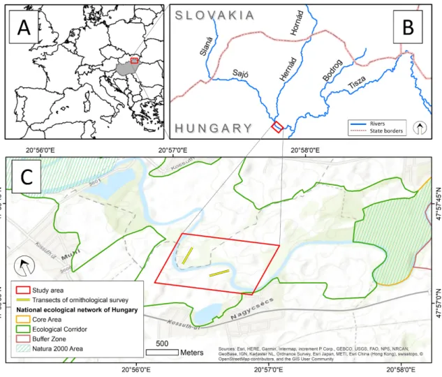
The Hungarian National Ecological Network (Phase 2) had been established between 1999–2001 according to the legislation of the Pan-European Ecological Network (PEEN). The components of the network provide the following landscape element categories: well-known core-areas, ecological corridors, buffer zones and restoration areas [48]. Core areas provide the main habitats and genetic reserves while the strip-like ecological corridors serve as continuous habitats or chains linking the smaller and larger habitat patches together [49]. This study focuses on a selected 2.12 km long sub-reach of the SajóRiver consisting of three consecutive river bends near the town of Nagycsécs, Hungary (Figure1). The further calculations were performed on this 68.4 ha large rectangular area around the river channel. This sub-reach of SajóRiver can be considered as a free-forming meandering type located between major river engineering works both upstream and downstream. The study area as part of the SajóRiver floodplain belongs to the PEEN category of ecological corridors between two main Natura2000 areas.
Water2018,10, 1613 4 of 21
as Chenopodium album, Chenopodium ambrosioides, Bidens tripartitus, at their wet riverside edges Polygonum hydropier, Polygonum minus, Polygonum mite, Rorippa amphibia, Rumex crispus, and Rumex obtusifolius.
Perennial grasslands are dominated by diverse grass species like Phalaris arundinacea, Agrostis stolonifera, Alopecurus pratensis, and Agropyron repens, varying by land use and duration of floods. In forest and bush patches grow Salix purpurea, Salix triandra, Salix alba, and Populus spp.
Figure 1. Overview of the study area. (A) Location of the study area in Europe; (B) Location of the main rivers in the region of study area; (C) Detailed overview of the selected sub-reach of Sajó River.
2.2. Datasets
This study aims to develop a spatiotemporal analysis on the river channel development and the ecological diversity based on a set of aerial imagery in 10 different time periods (Table 1). A set of black/white military-based historical aerial photographs of the study were available from the year of 1952, 1956, 1975 and 1988 given by the Hungarian Military History Museum. The archive aerial imagery was scanned in 600 dpi resolution and then orthorectified using the ERDAS Imagine software. However, orthophotographs of 2011 were used as a reference (datum: Hungarian HD72/EOV), but we included Topographical maps of 1980 as well since there were few field objects on the aerial imagery between 1952 and 1988, that w not possible to identify on the orthophotographs of 2011. During the process, 15–20 ground control points (GCP) were used for each image to provide accurate georeferencing. The RMSE (Root Mean Square Error) values varied between 3.4 to 6.7 m with an average of 4.8 m. We purchased digital colour orthophotographs of 2000, 2005 and 2011. The scale range of the aerial imagery and orthophotographs were found between 1:7000 and 1:12,000.
After 2011, there were no official orthophotographs available from the study area. Nowadays, UAVs offer a valuable solution to produce high-resolution aerial imagery from a few km2 large areas [50,51];
thus they are widely used for mapping wetland areas, especially for disaster management [52,53].
Figure 1.Overview of the study area. (A) Location of the study area in Europe; (B) Location of the main rivers in the region of study area; (C) Detailed overview of the selected sub-reach of SajóRiver.
We observed that the land mosaic of the study area was represented by a patch-complex consisting of bare surfaces, perennial grasslands, forests and bushes, the river channel, arable lands, and settlements. Bare plots, grasslands, and arboreal vegetation were considered as patches connected to each other by their own successive development controlled by the river channel changes and flood dynamic. On the other, arable lands and settlements were considered as mainly human-controlled elements of this structure. Bare surfaces meant patches not completely in a lack of vegetation, but with a low cover. Plant species of these sites are mainly disturbance-tolerant species such asChenopodium album,Chenopodium ambrosioides,Bidens tripartitus, at their wet riverside edgesPolygonum hydropier,Polygonum minus,Polygonum mite,Rorippa amphibia,Rumex crispus, and Rumex obtusifolius. Perennial grasslands are dominated by diverse grass species likePhalaris arundinacea, Agrostis stolonifera,Alopecurus pratensis, andAgropyron repens, varying by land use and duration of floods. In forest and bush patches growSalix purpurea,Salix triandra,Salix alba, andPopulusspp.
2.2. Datasets
This study aims to develop a spatiotemporal analysis on the river channel development and the ecological diversity based on a set of aerial imagery in 10 different time periods (Table1). A set of black/white military-based historical aerial photographs of the study were available from the year of 1952, 1956, 1975 and 1988 given by the Hungarian Military History Museum. The archive aerial imagery was scanned in 600 dpi resolution and then orthorectified using the ERDAS Imagine software. However, orthophotographs of 2011 were used as a reference (datum: Hungarian HD72/EOV), but we included
Water2018,10, 1613 5 of 21
Topographical maps of 1980 as well since there were few field objects on the aerial imagery between 1952 and 1988, that w not possible to identify on the orthophotographs of 2011. During the process, 15–20 ground control points (GCP) were used for each image to provide accurate georeferencing.
The RMSE (Root Mean Square Error) values varied between 3.4 to 6.7 m with an average of 4.8 m.
We purchased digital colour orthophotographs of 2000, 2005 and 2011. The scale range of the aerial imagery and orthophotographs were found between 1:7000 and 1:12,000. After 2011, there were no official orthophotographs available from the study area. Nowadays, UAVs offer a valuable solution to produce high-resolution aerial imagery from a few km2large areas [50,51]; thus they are widely used for mapping wetland areas, especially for disaster management [52,53]. UAV-based surveys were conducted in 2015 by using DJI Phantom drones in order to provide orthophotographs for 2015, 2016 and 2017. Each flight was performed at low-flow conditions while, at least, 20 GCPs were measured by a Stonex RTK-GPS system. UAV image acquisition was performed at 150 m A.G.L. with 75% frontlap and sidelap between flight paths to provide a ground resolution of 0.07 to 0.09 m. Agisoft Photoscan software was used for the photogrammetric processing and the creation of orthophotographs with an overall accuracy of around 0.05 m.
Table 1.Basic parameters of aerial imagery and orthophotographs used in this study.
Year Number of Images Type Scale Resolution (m) RMSE (m)
1952 22 B/W Aerial photo 1:7000 0.5 2.7
1956 18 B/W Aerial photo 1.7000 0.5 3.9
1975 15 B/W Aerial photo 1:12,000 0.5 2.2
1988 17 B/W Aerial photo 1:12,000 0.5 2.8
2000 22 Ortophoto 1:10,000 0.5 -
2005 22 Ortophoto 1:10,000 0.5 -
2011 22 Ortophoto 1:10,000 0.4 -
2015 1 UAV-Orthophoto 1:7498 0.09 0.05
2016 1 UAV-Orthophoto 1:8272 0.07 0.05
2017 1 UAV-Orthophoto 1:7669 0.07 0.05
2.3. Indices of River Channel Development
In order to quantify the extent of degradation by the lateral bank erosion, overlays of pairs (Figure2) related to consecutive time periods of the river channel polygons were composed [3]. In this research, we consider that understanding the area of accretion also plays a key role in the case of ecosystem diversity analysis. These two variables were derived at the same time. The crosshatched area represents that part of the floodplain where the two-channel planforms overlap and it appears that the channel did not change position, without any pronounced erosion or accretion.
Water 2018, 10, x 5 of 22
UAV-based surveys were conducted in 2015 by using DJI Phantom drones in order to provide orthophotographs for 2015, 2016 and 2017. Each flight was performed at low-flow conditions while, at least, 20 GCPs were measured by a Stonex RTK-GPS system. UAV image acquisition was performed at 150 m A.G.L. with 75% frontlap and sidelap between flight paths to provide a ground resolution of 0.07 to 0.09 m. Agisoft Photoscan software was used for the photogrammetric processing and the creation of orthophotographs with an overall accuracy of around 0.05 m.
Table 1. Basic parameters of aerial imagery and orthophotographs used in this study.
Year Number of Images Type Scale Resolution (m) RMSE (m)
1952 22 B/W Aerial photo 1:7000 0.5 2.7
1956 18 B/W Aerial photo 1.7000 0.5 3.9
1975 15 B/W Aerial photo 1:12,000 0.5 2.2
1988 17 B/W Aerial photo 1:12,000 0.5 2.8
2000 22 Ortophoto 1:10,000 0.5 -
2005 22 Ortophoto 1:10,000 0.5 -
2011 22 Ortophoto 1:10,000 0.4 -
2015 1 UAV-Orthophoto 1:7498 0.09 0.05
2016 1 UAV-Orthophoto 1:8272 0.07 0.05
2017 1 UAV-Orthophoto 1:7669 0.07 0.05
2.3. Indices of River Channel Development
In order to quantify the extent of degradation by the lateral bank erosion, overlays of pairs (Figure 2) related to consecutive time periods of the river channel polygons were composed [3]. In this research, we consider that understanding the area of accretion also plays a key role in the case of ecosystem diversity analysis. These two variables were derived at the same time. The crosshatched area represents that part of the floodplain where the two-channel planforms overlap and it appears that the channel did not change position, without any pronounced erosion or accretion.
Figure 2. Methodology for calculating areas of erosion and accretion.
The value of sinuosity index (SI) was calculated as the ratio of channel length to valley length [54]; consequently, not just the areal but morphological trend of river channel development could be assessed too. We determined the channel length as the length of channel centerline while valley length was measured as the distance between the point where Sajó River crosses the Hungarian border and the point of the Tisza River confluence. We calculated total SI values for each investigated time-period. We determined the mean channel migration rate based on polygons drawn by the overlapping centerlines in each consecutive time periods. The mean lateral channel shift is a ratio of polygon area and the half of the polygon perimeter [55]. Regarding erosion/accretion and channel shift, we normalized the values by the number of years covering each different periods.
We identified the meander parameters e.g., chord length (straight line distance between two inflexion points; but this value is not equal with meander wavelength, that is the straight line distance of two consecutive meander apexes of the same side of the river banks), amplitude, the width-
Figure 2.Methodology for calculating areas of erosion and accretion.
The value of sinuosity index (SI) was calculated as the ratio of channel length to valley length [54];
consequently, not just the areal but morphological trend of river channel development could be
assessed too. We determined the channel length as the length of channel centerline while valley length was measured as the distance between the point where SajóRiver crosses the Hungarian border and the point of the Tisza River confluence. We calculated total SI values for each investigated time-period. We determined the mean channel migration rate based on polygons drawn by the overlapping centerlines in each consecutive time periods. The mean lateral channel shift is a ratio of polygon area and the half of the polygon perimeter [55]. Regarding erosion/accretion and channel shift, we normalized the values by the number of years covering each different periods.
We identified the meander parameters e.g., chord length (straight line distance between two inflexion points; but this value is not equal with meander wavelength, that is the straight line distance of two consecutive meander apexes of the same side of the river banks), amplitude, the width-normalized radius of curvature (R/w). Channel widths were also determined in every 20 m along the centerlines of each time periods; therefore, a detailed mean channel width was given at the end.
2.4. Ornithological Survey
The avifauna of the study area via transect and point count surveys during the breeding season of 2018 was assessed. We selected two 200 m long line transects traversing the recently deposited areas as well as an observation point along an eroding section of the river to be able to detect birds along the full length of the study area. The transects were 500 m apart, while the point was 225 m and 580 m from the transects. We conducted the survey on 26 June between 10:00 a.m. and 12:40 p.m. Each transect survey lasted for 30 min and the point count for 20 min during which the observer recorded all species seen or heard in the vicinity of the river channel and the surrounding floodplain that are potentially using the habitat (i.e., not just flying over it at a high altitude).
We also quantified the size of the sand martin colonies of the eroding river banks of the study area from photo-mosaics. We applied close-range terrestrial photogrammetry to compose the mosaic view of the eroding river bank. For this purpose, a Nikon D5300 camera with a 70–300 mm tele-objective lens was used to capture the necessary photo-sequences of 218 images from tripod stands from the opposite side of the river. The datasets were processed in Agisoft Photoscan software. We printed coded targets of the software in A4 size in order to place them on the bank edges. We measured their precise coordinates by Stonex RTK-GPS system in order to provide a reliable scaling of the mosaic in Agisoft Photoscan.
2.5. Landscape Metrics
Class and landscape level landscape metrics to reveal the ecological features and processes along the changing river channel were applied. Initially, landscape patches were manually vectorized with a scale of 1:1000 in ArcGIS 10.3 on the aerial imagery in each investigated time-period. During the process, we have delineated the following land use categories: forests and bushes, grasslands, arable lands, bare point bar surfaces, settlement and the river channel itself (Figure3). Aerial photographs of 1952, 1956, 1975 and 1988 are black and white ones and sometimes the quality is far from good, however, these photographs ensure a larger time range to monitor the changes. Land cover classes had to be consistent; therefore, we merged the bushes and trees of forests. We decided to apply this approach considering the four stage successional model of Corenblit [56]. In our case bare surfaces represents the vegetation recruitment phase, grasslands are in phase of vegetation establishment and succession continues with development of bushes and forests, which consists the same spectrum of species but in different age and development phase. The river channel itself is the main factor for diaspore dispersion. Arable lands and settlements are totally controlled by the society, until the migration of the river channel does not alter this situation and shift them to a previous phase of succession.
Water2018,10, 1613 7 of 21
Water 2018, 10, x 7 of 22
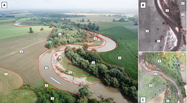
Figure 3. Aerial overview of the study area with the different land use categories (1—forests and bushes; 2—grasslands; 3—arable lands; 4—bar surfaces; 5—river channel). (A) Oblique aerial photo by L.B., 11 June 2017; (B) Black & White archive aerial photo from 1975; (C) UAV-based orthophoto from 2017.
We concentrated on the metrics which reflect the diversity of the floodplain and its environments:
• Patch Density (PD): we calculated the index on landscape level as the number of patches per unit area (Equation (1)).
= (10,000)(100) (1)
where N is the number of patches in the landscape, and A is the total area (m2), and the outcome is expressed in number. per 100 ha−1 [57].
• Interspersion and Juxtaposition Index (IJI): we calculated the index on landscape level as the function of observed interspersion and the maximum possible interspersion for the given number of patch types (Equation (2)).
IJI =− ∑ ∑ ( ) × ( ) ( − 1)
2 (2)
where Eik: the total edge between patch types i and k; m: number of patch types.
IJI is expressed in per cent (0–100); low values indicate unevenly distributed or isolated patches in the area, the largest value is acquired when all patch types have a common edge with all possible other patch types [57,58].
• Shannon’s Diversity Index (SHDI): We calculated the index on landscape level as the sum of the proportional abundance of each patch type multiplied by that proportions (Equation (3)).
SHDI = − ∑ ( . ) (3)
where Pi is the proportion of the landscape occupied by the patch type i. When the landscape is occupied by only one patch SHDI = 0 and increases with the number of patch types and their proportional area without upper limit [57,59].
• Class Area of the forests (CA_F): we considered the forests’ area as the indicator of landscape change (in the initial phase, in 1956, there were only a few small patches and later, with the river Figure 3. Aerial overview of the study area with the different land use categories (1—forests and bushes; 2—grasslands; 3—arable lands; 4—bar surfaces; 5—river channel). (A) Oblique aerial photo by L.B., 11 June 2017; (B) Black & White archive aerial photo from 1975; (C) UAV-based orthophoto from 2017.
In order to quantify and evaluate the direct changes in land cover and the transformation of land patches related to vegetation succession, channel migration or human agricultural management, we calculated a confusion matrix based on the vectorized land cover files in Idrisi software. In these tables, the diagonal values related to a pair of a given land cover category represents the proportion of area where no changes were found. The columns represents the initial land cover category while the rows will define the land cover categories that the given column category were transformed into.
The values represents their proportion from the total area.
We concentrated on the metrics which reflect the diversity of the floodplain and its environments:
• Patch Density (PD): we calculated the index on landscape level as the number of patches per unit area (Equation (1)).
PD= N
A(10, 000)(100) (1)
whereNis the number of patches in the landscape, andAis the total area (m2), and the outcome is expressed in number.per 100 ha−1[57].
• Interspersion and Juxtaposition Index (IJI): we calculated the index on landscape level as the function of observed interspersion and the maximum possible interspersion for the given number of patch types (Equation (2)).
IJI= −∑mi=1∑mk=i+1[(Eik)×ln(Eik)]
lnm(m−1)
2
(2)
whereEik: the total edge between patch typesiandk;m: number of patch types. IJI is expressed in per cent (0–100); low values indicate unevenly distributed or isolated patches in the area, the largest value is acquired when all patch types have a common edge with all possible other patch types [57,58].
• Shannon’s Diversity Index (SHDI): We calculated the index on landscape level as the sum of the proportional abundance of each patch type multiplied by that proportions (Equation (3)).
SHDI=−
∑
m i=1(Pi.lnPi) (3)
wherePiis the proportion of the landscape occupied by the patch typei. When the landscape is occupied by only one patch SHDI = 0 and increases with the number of patch types and their proportional area without upper limit [57,59].
• Class Area of the forests (CA_F): we considered the forests’ area as the indicator of landscape change (in the initial phase, in 1956, there were only a few small patches and later, with the river bed development, the area relevantly increased). The index was calculated as the proportion of the forest land cover type and the total area and was expressed in per cent.
2.6. Statistical Analysis
After the calculation of descriptive statistics, the connection between the indices of river channel development (Sinuosity—SI, Area of erosion—Er, Area of Accretion—Ar) and the landscape metrics was also investigated. Regression analysis and Principal Component Analysis (PCA) were applied.
While the regression analysis pointed on the changes directly with the given variables and provided valuable information on the temporal features and breakpoints of the surface development, PCA helped to identify the years when both the landscape and the river bed had deterministic relations.
Standardized PCA was conducted using the correlation matrix with Varimax rotation to gain orthogonal axes, i.e., non-correlating principal components (PCs) [60,61]. PD, CA_F, IJI, and SHDI landscape metrics and the Er, Acc and SI indices of riverbed development were involved.
Thus, it became possible to identify both the cross-connections among the variables and to visualize the dates of different stages of surface development on a biplot diagram. Model fit was controlled with the Root Mean Square Residual (RMSR), which is determined using the residuals of the original correlation matrix and the estimation of the PCA [62]. RMSR values of <0.05 indicates very good fit [63].
We applied the Jonckheere-Terpra test to reveal whether there was a trend in river channel change over the studied period. Statistical analysis was performed using the software Past 3.19 [64] and R 3.5 [65] by applying the psych [66] and GPArotation [67] packages; furthermore, the lattice [68], the clinfun [69] and ggplot2 [70] packages were applied for the data visualization.
3. Results
3.1. Changes in Land Cover and Channel Morphology
Detailed land cover changes based on the vectorization of the available aerial imagery are shown in Figure4. After a visual interpretation of the figure, it is clearly visible that significant changes occurred over the investigated periods (65 years). The channel developed at a remarkable rate developing three main meandering bends with high sinuosity.
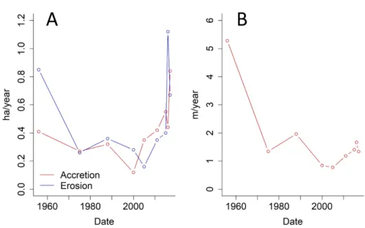
According to the results of the normalized erosion and accretion rates, the first period between 1952 and 1956 showed the second highest bank erosion (0.85 ha·year−1) rate (Figure5A). Bank erosion activity radically decreased with three times by 1975. It was followed by a gentle increase between 1975–1980 but after that, it decreased again and reached the lowest bank erosion rate (0.16 ha·year−1) in 2005. A notable increase started in 2010 with an outstanding maximum value of 1.12 ha·year−1 in the period of 2015–2016. Except for the first period (1952–1956), accretion rates followed closely the erosion rates; moreover, from the period of 2000–2005, except the above-mentioned extremely erosive year between 2015 and 2016, they exceeded their contribution over the eroded areas in the channel development. Lateral migration rates (Figure5B) primarily followed the trend of erosion rates as it started from a relatively high rate (5.3 m) of channel shift and decreased by 1975. Its minimum
Water2018,10, 1613 9 of 21
(0.8 m) was also found in 2005 then similarly started to increase, however, its peak of 2016 was not as outstanding, due to its erosion rates.
Water 2018, 10, x 9 of 22
Figure 4. Land cover changes of the study area.
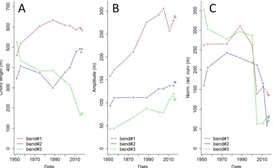
The parameters of meander evolution are summarized in Figure 6. The chord length (Figure 6A) increased in Bend 1 from 460 m to 634 m until 1988 but it was followed by a slight decrease. However, Bend 2 showed the opposite trend as it decreased to 299 m by 1988, but then the chord length increased intensely with almost 200 m by 2017. Bend 3 decreased monotonously and the total change was almost 350 m from 1952 to 2017. Amplitude (Figure 6B) increased in all the bends but the expansion of Bend 1 was almost two times higher (+127.49 m) than the others. The change in width- normalized radius of curvature (Figure 6C) showed a similar increase as it was in chord length between 1952 and 1988 but it was also found at Bend 3 as well. It was followed by an intensive decrease, especially in Bend 3.
Figure 5. (A) Time series of normalized accretion and erosion rates in the studied period; (B) Time series of mean lateral channel shift rates in the studied period.
Figure 4.Land cover changes of the study area.
Water 2018, 10, x 9 of 22
Figure 4. Land cover changes of the study area.
The parameters of meander evolution are summarized in Figure 6. The chord length (Figure 6A) increased in Bend 1 from 460 m to 634 m until 1988 but it was followed by a slight decrease. However, Bend 2 showed the opposite trend as it decreased to 299 m by 1988, but then the chord length increased intensely with almost 200 m by 2017. Bend 3 decreased monotonously and the total change was almost 350 m from 1952 to 2017. Amplitude (Figure 6B) increased in all the bends but the expansion of Bend 1 was almost two times higher (+127.49 m) than the others. The change in width- normalized radius of curvature (Figure 6C) showed a similar increase as it was in chord length between 1952 and 1988 but it was also found at Bend 3 as well. It was followed by an intensive decrease, especially in Bend 3.
Figure 5. (A) Time series of normalized accretion and erosion rates in the studied period; (B) Time series of mean lateral channel shift rates in the studied period.
Figure 5.(A) Time series of normalized accretion and erosion rates in the studied period; (B) Time series of mean lateral channel shift rates in the studied period.
The parameters of meander evolution are summarized in Figure6. The chord length (Figure6A) increased in Bend 1 from 460 m to 634 m until 1988 but it was followed by a slight decrease. However, Bend 2 showed the opposite trend as it decreased to 299 m by 1988, but then the chord length increased intensely with almost 200 m by 2017. Bend 3 decreased monotonously and the total change was almost 350 m from 1952 to 2017. Amplitude (Figure6B) increased in all the bends but the expansion of Bend 1
was almost two times higher (+127.49 m) than the others. The change in width-normalized radius of curvature (Figure6C) showed a similar increase as it was in chord length between 1952 and 1988 but it was also found at Bend 3 as well. It was followed by an intensive decrease, especially in Bend 3.Water 2018, 10, x 10 of 22
Figure 6. Parameters of meander evolution and channel shift (A) chord length (m); (B) bend amplitude (m); (C) width-normalized radius of curvature (m).
We justified a significant decreasing trend in case of river channel width (Figure 7) as a function of time (J-T statistic = 80298; p = 0.0004) and there was a negative correlation between the mean channel width and sinuosity (r = −0.93, p < 0.001).
Figure 7. Changes in the mean channel width.
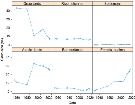
Land cover changes can be divided into two groups: (1) settlement, river channel and point bars where the changes were minimal (the area was more or less constant but the patches had spatial changes); (2) arable land, grassland and forests where the changes were relevant (these patch types turned into another, at least, partly). The area of grasslands decreased transforming into arable land and forest (Figure 8). The extent of the forests and bushes increased by 25% since the share of grasslands showed a decrease in similar rate and bare surfaces were not changed considerably. The
Figure 6.Parameters of meander evolution and channel shift (A) chord length (m); (B) bend amplitude (m); (C) width-normalized radius of curvature (m).
We justified a significant decreasing trend in case of river channel width (Figure7) as a function of time (J-T statistic = 80298;p= 0.0004) and there was a negative correlation between the mean channel width and sinuosity (r=−0.93,p< 0.001).
Water 2018, 10, x 10 of 22
Figure 6. Parameters of meander evolution and channel shift (A) chord length (m); (B) bend amplitude (m); (C) width-normalized radius of curvature (m).
We justified a significant decreasing trend in case of river channel width (Figure 7) as a function of time (J-T statistic = 80298; p = 0.0004) and there was a negative correlation between the mean channel width and sinuosity (r = −0.93, p < 0.001).
Figure 7. Changes in the mean channel width.
Land cover changes can be divided into two groups: (1) settlement, river channel and point bars where the changes were minimal (the area was more or less constant but the patches had spatial changes); (2) arable land, grassland and forests where the changes were relevant (these patch types turned into another, at least, partly). The area of grasslands decreased transforming into arable land and forest (Figure 8). The extent of the forests and bushes increased by 25% since the share of grasslands showed a decrease in similar rate and bare surfaces were not changed considerably. The
Figure 7.Changes in the mean channel width.
Land cover changes can be divided into two groups: (1) settlement, river channel and point bars where the changes were minimal (the area was more or less constant but the patches had spatial
Water2018,10, 1613 11 of 21
changes); (2) arable land, grassland and forests where the changes were relevant (these patch types turned into another, at least, partly). The area of grasslands decreased transforming into arable land and forest (Figure8). The extent of the forests and bushes increased by 25% since the share of grasslands showed a decrease in similar rate and bare surfaces were not changed considerably.
The extent of human-controlled arable lands was increased at the beginning but slightly decreased in the last decades. Extents of the river channel and settlement were not changed considerably.
Water 2018, 10, x 11 of 22
extent of human-controlled arable lands was increased at the beginning but slightly decreased in the last decades. Extents of the river channel and settlement were not changed considerably.
Figure 8. Changes in land cover over the studied period by patch types.
The detailed contingency tables of land cover changes between each consecutive time periods were summarized and available in Supplementary file 1. In Table 2, we presented the changes of selected pairs of land use category transformations that showed higher conversion proportions. The first four rows represent the successional phases that follow the channel migration: The second highest transformation rates were connected to the transformation from former river channel to bar surfaces. It was followed by colonization of the bar surfaces by grasslands where the transformation rates were found also lower and totally stopped by 2005. However, generally, direct transformation from bar surfaces to forests showed some higher values but it could have been expressed by the longer time periods covered. The highest transformation rates were found in the transformation from grasslands to forests. The last four rows represents transformation categories that were controlled by the channel migration and bank retreat except the changes from grasslands to arable lands. This type also resulted in an outstanding proportion (0.326) between 1975 and 1988 and it radically decreased afterwards.
Table 2. Conversion matrix (changes in percent) of LC categories in the investigated periods.
Conversion Type
1952–1956 1956–1975 1975–1988 1988–2000 2000–2005 2005–2011 2011–2015 2015–2016 2016–2017 Initial Final
RC BS 0.016 0.019 0.028 0.007 0.013 0.014 0.018 0.005 0.004 BS G 0.008 0.016 0.005 0.008 0.002 0 0 0 0 BS F 0.002 0.005 0.021 0.026 0.012 0.013 0.006 0.005 0.009
G F 0.010 0.030 0.049 0.008 0.023 0.088 0.030 0.014 0.007 G RC 0.008 0.025 0.042 0 0.001 0.005 0.001 0 0 G AL 0.001 0.008 0.326 0.002 0.006 0.010 0.007 0.001 0.001 F RC 0.001 0.002 0.004 0.007 0.003 0.004 0.004 0.006 0.002 AL RC 0.011 0.011 0 0.017 0.006 0.018 0.015 0.004 0.004
AL—Arable lands, BS—Bar surfaces, F—Forests, G—Grasslands, RC—River channel.
Figure 8.Changes in land cover over the studied period by patch types.
The detailed contingency tables of land cover changes between each consecutive time periods were summarized and available in Supplementary File S1. In Table2, we presented the changes of selected pairs of land use category transformations that showed higher conversion proportions. The first four rows represent the successional phases that follow the channel migration: The second highest transformation rates were connected to the transformation from former river channel to bar surfaces.
It was followed by colonization of the bar surfaces by grasslands where the transformation rates were found also lower and totally stopped by 2005. However, generally, direct transformation from bar surfaces to forests showed some higher values but it could have been expressed by the longer time periods covered. The highest transformation rates were found in the transformation from grasslands to forests. The last four rows represents transformation categories that were controlled by the channel migration and bank retreat except the changes from grasslands to arable lands. This type also resulted in an outstanding proportion (0.326) between 1975 and 1988 and it radically decreased afterwards.
Table 2.Conversion matrix (changes in percent) of LC categories in the investigated periods.
Conversion Type
1952–1956 1956–1975 1975–1988 1988–2000 2000–2005 2005–2011 2011–2015 2015–2016 2016–2017 Initial Final
RC BS 0.016 0.019 0.028 0.007 0.013 0.014 0.018 0.005 0.004
BS G 0.008 0.016 0.005 0.008 0.002 0 0 0 0
BS F 0.002 0.005 0.021 0.026 0.012 0.013 0.006 0.005 0.009
G F 0.010 0.030 0.049 0.008 0.023 0.088 0.030 0.014 0.007
G RC 0.008 0.025 0.042 0 0.001 0.005 0.001 0 0
G AL 0.001 0.008 0.326 0.002 0.006 0.010 0.007 0.001 0.001
F RC 0.001 0.002 0.004 0.007 0.003 0.004 0.004 0.006 0.002
AL RC 0.011 0.011 0 0.017 0.006 0.018 0.015 0.004 0.004
AL—Arable lands, BS—Bar surfaces, F—Forests, G—Grasslands, RC—River channel.
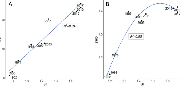
A linear relationship between the increase of forest areas and the SI (R2= 0.94,p< 0.001; Figure9A) was revealed. At the first date of the study period (1956), only a few patches of the forest were observed, which reached a 25% proportion till 2017; besides, SI indicated a straight river channel section in 1956 and it became a complex form up to 2017. Thus, the forest areas increased directly as the river channel transformed and appropriate areas developed in the floodplain.
A linear relationship between the increase of forest areas and the SI (R2 = 0.94, p < 0.001; Figure 9A) was revealed. At the first date of the study period (1956), only a few patches of the forest were observed, which reached a 25% proportion till 2017; besides, SI indicated a straight river channel section in 1956 and it became a complex form up to 2017. Thus, the forest areas increased directly as the river channel transformed and appropriate areas developed in the floodplain.
Figure 9. Sinuosity as independent factor of land cover changes and landscape diversity in the study area. (A) The relationship between the SI (Sinuosity Index) and CAF (Class area of Forests); (B) Relationship between the SI (Sinuosity Index) and SHDI (Shannon’s Diversity Index) metrics.
There was a significant connection between the SI and SHDI variables (R2 = 0.93, p < 0.001).
However, unlike in the case of forest areas, the connection was not linear (Figure 7B); a second-order polynomial regression indicated that there was a change in the trend after 2011: next years (2015–
2017) were outside of the linear trend and the curve showed saturation; moreover, there was a small decrease in the diversity in 2017.
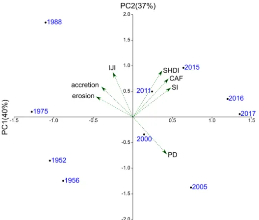
PCA explained the 94% of the total variance. Three principal components (PC) were justified by the RMRS (0.03). PC1 correlated with the Er (Area of Erosion), Acc (Area of Accumulation) and PD (Patch Density) explaining 40% of the total variance. PC2 correlated with the SI, SHDI, and CAF and accounted for 37% of the total variance, while PC3 was formed by solely the IJI having 18% in the explanation of the total variance. Acc and Er correlated with the PD and SI with the SHDI and CAF.
The ordination diagram showed that years formed two distinct groups differentiated by the Er, Acc and PD indices (Figure 10). The first group was situated in the negative part of the diagram, and the second, with a larger range, in the positive part. Considering the vertical axis (PC2), the distribution followed a monotonous increasing trend between 1956 and 1988 but it became sparse after 2000 with 2005 having the lowest value and after another increase, it started to decrease from 2015.
Figure 9. Sinuosity as independent factor of land cover changes and landscape diversity in the study area. (A) The relationship between the SI (Sinuosity Index) and CAF (Class area of Forests);
(B) Relationship between the SI (Sinuosity Index) and SHDI (Shannon’s Diversity Index) metrics.
There was a significant connection between the SI and SHDI variables (R2 = 0.93,p< 0.001).
However, unlike in the case of forest areas, the connection was not linear (Figure7B); a second-order polynomial regression indicated that there was a change in the trend after 2011: next years (2015–2017) were outside of the linear trend and the curve showed saturation; moreover, there was a small decrease in the diversity in 2017.
PCA explained the 94% of the total variance. Three principal components (PC) were justified by the RMRS (0.03). PC1 correlated with the Er (Area of Erosion), Acc (Area of Accumulation) and PD (Patch Density) explaining 40% of the total variance. PC2 correlated with the SI, SHDI, and CAF and accounted for 37% of the total variance, while PC3 was formed by solely the IJI having 18% in the explanation of the total variance. Acc and Er correlated with the PD and SI with the SHDI and CAF.
The ordination diagram showed that years formed two distinct groups differentiated by the Er, Acc and PD indices (Figure10). The first group was situated in the negative part of the diagram, and the second, with a larger range, in the positive part. Considering the vertical axis (PC2), the distribution followed a monotonous increasing trend between 1956 and 1988 but it became sparse after 2000 with 2005 having the lowest value and after another increase, it started to decrease from 2015.
3.2. Avifauna
Since the biodiversity can be affected by the different land cover and morphological river changes, we surveyed the avifauna as a possible bioindicator. Result of the snapshot faunistic survey is shown in Table3. A total of 26 species were detected breeding or using the habitat during the breeding season, of which 23 are protected under the Hungarian law including the strictly protected European bee-eater (Merops apiaster) [71].
Water2018,10, 1613 13 of 21
Water 2018, 10, x 13 of 22
Figure 10. Biplot of the PCA model conducted with the landscape metrics and river channel development indices (dashed arrows: involved variables).
3.2. Avifauna
Since the biodiversity can be affected by the different land cover and morphological river changes, we surveyed the avifauna as a possible bioindicator. Result of the snapshot faunistic survey is shown in Table 3. A total of 26 species were detected breeding or using the habitat during the breeding season, of which 23 are protected under the Hungarian law including the strictly protected European bee-eater (Merops apiaster) [71].
Figure 10. Biplot of the PCA model conducted with the landscape metrics and river channel development indices (dashed arrows: involved variables).
Table 3.List of bird species seen and/or heard during the censuses listed in taxonomic order.
Common Name Scientific Name
1 Grey heron Ardea cinerea
2 Common buzzard Buteo buteo
3 Common kestrel Falco tinnunculus
4 Eurasian hobby Falco subbuteo
5 Common pheasant Phasianus colchicus
6 Common sandpiper Tringa hypoleucos
7 Woodpigeon Columba palumbus
8 Turtle dove Streptopelia turtur
9 Common cuckoo Cuculus canorus
10 Common kingfisher Alcedo atthis
11 European bee-eater Merops apiaster
12 Green woodpecker Picus viridis
13 Great spotted woodpecker Dendrocopus major
14 Sand martin Riparia riparia
15 Common blackbird Turdus merula
16 River warbler Locustella fluviatilis 17 Eurasian blackcap Sylvia atricapilla
18 Chiffchaff Phylloscopus collybita
19 Great tit Parus major
20 Common starling Sturnus vulgaris
21 Golden oriole Oriolus oriolus
22 Eurasian jay Garrulus glandarius
23 Hooded Crow Corvus cornix
24 Common chaffinch Fringilla coelebs
25 European greenfinch Carduelis chloris 26 European goldfinch Carduelis carduelis
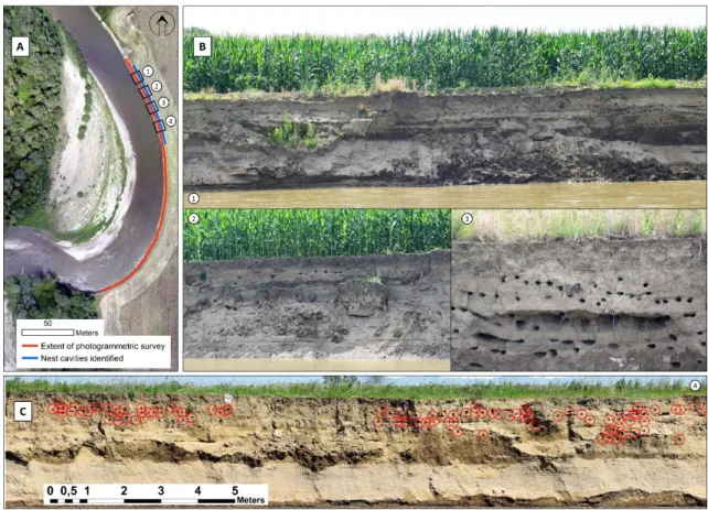
The nest cavities of both the bee-eater and the steeply declining Sand martin (Riparia riparia) was found along the eroding section of the SajóRiver bank. Approximately, 80–100 pairs of sand martins were feeding young at the time of the survey at the focal section of the river. However, based on the number of visible nest cavities (Figure11), the two colonies could have consisted of a total of 446
breeding pairs.Water 2018, 10, x 15 of 22
Figure 11. Nest cavities along the eroding river banks of Sajó River at the study area. (A) The overview of the cavities; (B) Examples of cavities along the recently eroded slump blocks; (C) Red circles indicates the cavities identified on one part of the mosaic.
4. Discussion
Fluvial morphological changes are able to generate intensive modifications, which can affect hydrological processes and, even, biodiversity. One clear example is the Sajó River, which was assessed in this research. Sajó River itself is regulated only in particular reaches, but its morphological evolution is affected by the Tisza River. Sajó River as a tributary joins Tisza River and the study area is located only about 20 km upstream from the confluence, which is strongly affects the sediment transport and channel development of the studied Sajó River sub-reach. The Tisza was regulated during the second half of the 19th century, and as a result of these regulations, its riverbed was incised for its straightened channel and increased energy [42,43]. This process could be also responsible for the morphological changes of Sajó River. The characteristics of Tisza channel development basically changed after the construction dams on Tisza River, both on upstream (1954, Tiszalök) and on downstream (1978, Kisköre) sections around the firth of Sajó. The establishment of these dams could cause a reduction of sediment supply [54] which generally leads to further channel incision.
However, we determined the narrowing (Figure 7), and therefore, similarly to Tisza River, a possible incision, of the Sajó River but its channel started to develop in a different way, namely increased meandering started instead of a former incision, which has diverse effects on land cover, conservational value and productivity on surrounding landscape [72].
Morphological changes allow registering high rates of bank erosion, which in similar investigations in other European rivers, was also calculated [3,73,74]; however, the extent of arable lands lost by lateral erosion is not an outstanding value compared to other rivers with similar geomorphological patterns [75]. In this way, it would be a great opportunity to include in future investigations the correlation between these morphological alterations, the changes in the biodiversity and the bank erosion rates.
Figure 11.Nest cavities along the eroding river banks of SajóRiver at the study area. (A) The overview of the cavities; (B) Examples of cavities along the recently eroded slump blocks; (C) Red circles indicates the cavities identified on one part of the mosaic.
4. Discussion
Fluvial morphological changes are able to generate intensive modifications, which can affect hydrological processes and, even, biodiversity. One clear example is the SajóRiver, which was assessed in this research. SajóRiver itself is regulated only in particular reaches, but its morphological evolution is affected by the Tisza River. SajóRiver as a tributary joins Tisza River and the study area is located only about 20 km upstream from the confluence, which is strongly affects the sediment transport and channel development of the studied SajóRiver sub-reach. The Tisza was regulated during the second half of the 19th century, and as a result of these regulations, its riverbed was incised for its straightened channel and increased energy [42,43]. This process could be also responsible for the morphological changes of SajóRiver. The characteristics of Tisza channel development basically changed after the construction dams on Tisza River, both on upstream (1954, Tiszalök) and on downstream (1978, Kisköre) sections around the firth of Sajó. The establishment of these dams could cause a reduction of sediment supply [54] which generally leads to further channel incision. However, we determined the narrowing (Figure7), and therefore, similarly to Tisza River, a possible incision, of the SajóRiver but its channel started to develop in a different way, namely increased meandering started instead of a former incision, which has diverse effects on land cover, conservational value and productivity on surrounding landscape [72].
Water2018,10, 1613 15 of 21
Morphological changes allow registering high rates of bank erosion, which in similar investigations in other European rivers, was also calculated [3,73,74]; however, the extent of arable lands lost by lateral erosion is not an outstanding value compared to other rivers with similar geomorphological patterns [75]. In this way, it would be a great opportunity to include in future investigations the correlation between these morphological alterations, the changes in the biodiversity and the bank erosion rates.
It is notable that the accretion of the river bank mainly followed the rate of eroding outer banks; therefore, new bare point bar surfaces had been developed in a short time period. Although these surfaces are not valuable ecologically, at the beginning phase, they represent potential future habitats [74]; our study pointed out that in case the vegetation can rapidly occupy the area, then the process can increase the extent of habitat in the ecological corridors. Moreover, the studied sub-reach is situated between two Natura2000 areas, thus, channel migration can enhance the habitat diversity and species connectivity between these sub-groups of the ecological network, that strengthen the role of an ecological corridor, as a possible compensation of the land degradation processes.
The majority of previous studies were focusing on the extensive negative effects of river bank erosion i.e., spreading pollutants from upstream reservoirs or remobilizing heavy metal contaminants [76–78] but only a few discuss their ecological consequences. In some cases, under different climate conditions, the lateral shifts of river channels rapidly decrease the biodiversity of the neighbouring flora and fauna [79] but in this case, it affects only agricultural areas. In our study, we demonstrated an opposite dynamic: How the process can be valuable. Regarding the changes in landscape metrics, as SI values increased, the forest areas (CA-F) also increased. SI reflected how the planform of the river channel was developed, and the positive connection with the forest areas indicate that instead of the arable lands, a natural afforestation process was initiated. Small grassland patches can be merged into forest cover without appropriate management [80] but in this case, the increase of SI provided the criteria of the forest cover extension. The newly developed point bars were occupied by plants (firstly with herbaceous plants) and later became forested following a successional process.
Diversity did not follow the linear trend because the area of the forests reached a threshold when the further increase did not increase the diversity of the mosaic of land cover patches (Figure9). This is the explanation of the two kinds of the relationship of the SI with the landscape metrics. The analysis on the conversion matrix between land cover categories showed higher values on the changes related to vegetation succession phases while the lower values were found in connection with the channel migration. However, we found outstanding transformation from grasslands to arable lands between 1975 and 1980 but this can be clearly explained by human intervention on the land management.
Multivariate analysis revealed that 1956–1988 period had rather similar features considering the erosion-accretion processes and the PD, and there was another group of years between 2000 and 2017 that can be distinguished according to the remaining variables. However, considering the results of PCA, SI, SHDI, and CA_F variables differentiated the points a sparse distribution: As the erosion and accretion processes increased or decreased, or were larger or smaller compared to each other, the forest areas and the diversity also reacted differently. This process became the major regulator of the ecological process from 1988 to 2000 when the river channel development reached SI = 1.4 and in 2015 when it reached SI = 1.6, the pace of the lateral movement slowed down. At the beginning of meander development, the chord length remains stable and an extension, with increasing amplitude, occurs [11]. We observed similar changes along the studied SajóRiver reach since the chord lengths showed only minor changes until 1975 from where both increase (bend 2) and decrease (bend 1, 3) took place. According to [13] the decreasing normalized curvature (R/w) accelerates the channel migration as it was also found (Figures5b and6c) in the studied SajóRiver reach. The proportion of the forests increased from 1 to 25%, and, what is important, these areas were constant (if a patch type transformed into forest, most of the area remained forest in the consecutive years, too), while the grasslands, arable lands, and especially the point bars changed in spatial terms (changes can occur back and forth, or the formation and diminishing is a common process).
The development of successional riparian and fluvial forests on recently deposited point bars significantly increases biodiversity locally [81] but more importantly, it facilitates the movement of organisms across an otherwise cultivated and homogenous landscape, thus, allows the maintenance of gene flow between meta-populations. Indeed, the classification of the study area is “ecological corridor” within the National Ecological Network, which connects ecologically important core areas along the river. The avifauna of the study area is similar to communities detected along with other reaches of the river over two decades ago [82] suggesting that the newly formed habitats are quickly colonized by protected species from nearby areas.
The eroding banks provide important nesting sites for colonies of protected and regionally declining migratory bird species such as the sand martin and the European bee-eater [83] further increasing the ecological importance of the new habitats created by this dynamic river. In fact, an effective way to improve the availability of nesting sites and facilitate the recolonization of an area by sand martins is the removal of bank erosion control projects from heavily regulated river channels [84].
This may be particularly important for maintaining viable populations of sand martins in agricultural landscapes as these birds usually do not reuse their nests from previous years to avoid the costs of heavy infestation with parasites [85,86], rather select nesting sites along river banks and sand quarries where periodically renewing vertical surfaces are available at the beginning of the nesting season.
Eroding river banks at our study area provide just that, the continuous renewal of this critical resource, the nesting site, which often limits the distribution of both sand martins and bee-eaters [71,85].
The increase in the extent of the most stable successive landscape element (forests) and a decrease of elements in middle-phase of succession (grasslands) suggest that the land-mosaic alteration during the investigated time resulted in higher diversity and stability. This process is important regarding laterally active channels; therefore, identification of the relationship between morphological changes in river channel and landscape evolution is vital [2,56]. Changes of arable lands could not be used as an indication for river development since it is controlled by human actions related to agricultural management. As a main controlling factor for successive landscape elements, the altered dynamic of meandering could be evaluated. Even if no relevant human interventions were present within the study area, the changes in meandering-dynamic can be highly influenced by the anthropogenic changes in the flood-dynamic of the main stem Tisza River. Decreasing agricultural productivity due to bank failures and channel shifting seems to be balanced by increasing habitat diversity by recent point bar deposits, succession areas, and bushes. Considering the increasing share of cultivated areas during last decades within a floodplain, which is part of a national ecological network, positive effects of the meandering of the river exceeds the negative effects of land loss and lateral erosion.
Another important topic to be assessed in the future would be the connectivity processes [87].
It is clear that the studied river and surrounding landscapes are connected by different processes such as nutrient transport or sediment mobilization, both of these are also conditioned by the vegetation colonization [88–90]. The application of modelling techniques and connectivity indexes allow us detecting how meandering is influenced by other dynamic fluxes such as agricultural fields [91] or urban areas [92] and at which level. Therefore, undoubtedly, understanding connectivity processes in the Sajóriver would help land plan managers and stakeholders to design correct and sustainable soil erosion control measures and water conservation practices, as other authors also confirmed in other degraded areas [93,94].
5. Conclusions
River channel development is a natural process, which usually considered to have a negative effect due to the damages caused to agriculture or infrastructure. Our hypothesis was that, besides the detrimental phase, there is also a positive effect because of the newly developed habitats on the opposite side of the river. We revealed that 65 years were enough to gain a new habitat system along the river as the linear channel formed into a meandering and more natural state. At the beginning phase, there were only a few patches of forests and the matrix had been dominated by the surrounding