1 Szabó, Beáta; Lengyel, Edina; Padisák, Judit; Stenger-Kovács, Csilla. Benthic diatom metacommunity across small freshwater lakes: driving mechanisms, β-diversity and ecological uniqueness. HYDROBIOLOGIA 828:
pp. 183-198. (2018)
Benthic diatom metacommunity across small freshwater lakes: driving mechanisms, β- 1
diversity and ecological uniqueness 2
3
Beáta Szabó1,2*, Edina Lengyel1, Judit Padisák1,2 Csilla Stenger-Kovács2 4
5
1MTA-PE Limnoecology Research Group, Hungarian Academy of Sciences, Egyetem str. 10, 6
H-8200 Veszprém, Hungary 7
2 University of Pannonia, Department of Limnology, Egyetem str. 10, H-8200 Veszprém, 8
Hungary 9
10
*corresponding author: e-mail: szabobea@almos.uni-pannon.hu, phone number: +36-88- 11
624337, ORCID: http://orcid.org/0000-0002-2972-0306 12
13
2 Abstract
14 15
In this study, driving forces and diversity patterns of a benthic diatom metacommunity across 16
small freshwater lakes exhibiting environmental heterogeneity were investigated.
17
Furthermore, local (LCBD) and species (SCBD) contributions to β-diversity and their driving 18
parameters were assessed with abundance- and incidence-based analyses. Our results revealed 19
that both spatial distance and environmental heterogeneity affected the community assembly, 20
which corresponds most to the mass-effect (ME) concept. This theory was confirmed by high 21
α-diversity of sampling sites, however, high overall β-diversity enhanced mainly by turnover 22
contradicted the ME paradigm. LCBD indices were affected by environmental variables 23
furthermore, LCBD and LCBD in terms of species replacement showed a strong positive 24
correlation. The ecologically most unique sites hosted relatively low species richness, and 25
common species with intermediate-sized or broad niches contributed mostly to the regional β- 26
diversity. However, abundance- and incidence-based calculations revealed different 27
relationships of SCBD with the species’ total abundance and the number of occupied sites.
28
Consequently, we favor the previous suggestions that comprehensive research focusing on 29
conservation should incorporate the investigation of LCBD, SCBD, species-rich sites and also 30
ecologically restricted species. Moreover, in assessing ecological uniqueness, both abundance 31
and binary data sets should be considered since they might shed light on distinct patterns.
32 33
Key words: assembly mechanisms, diversity patterns, ecological uniqueness, mass-effect, 34
species richness 35
36
3 Introduction
37
The current ecology- and conservation-oriented research tends to explore the possible causes 38
of community assembly by examining it at regional scale, rather than by only “snap-shot”
39
investigation of groups of biota within a given habitat. That is, studies focusing on 40
metacommunity processes as well as β-diversity and its components are gaining more and 41
more attention. Within the metacommunity framework (Leibold et al., 2004) four different 42
concepts can be distinguished in explaining the importance of local- (species’ competitive 43
abilities, demographic processes) and regional-scale (degree of environmental heterogeneity, 44
dispersal) processes. In the neutral theory (NT), species are assumed to be identical 45
concerning their interspecific interactions and response to any limiting factor; demographic 46
processes (birth-death rates) are stochastic; the environment is homogeneous in the region;
47
and species are limited in their dispersion. The patch dynamic (PD) archetype assumes that 48
the species’ relative competitive abilities depend on the local environmental conditions; the 49
population-level extinctions are stochastic due to the individual-level stochasticity; the 50
environment is completely homogeneous or spatial heterogeneity may occur in response to 51
the environment; dispersal is limited but interspecific differences in colonization abilities are 52
allowed. In the mass-effect (ME) concept, competitive abilities and birth-death rates are 53
assumed to be largely dependent on the local environment, which displays heterogeneous 54
patterns; species are able to persist in suboptimal localities if there is a sufficient immigration 55
from adjacent sites with high population growth. The species-sorting (SS) concept, similarly 56
to the ME, expects that the environment is heterogeneous, local conditions regulate the 57
competitive abilities of species and the demographic processes; dispersal is sufficient, thus 58
each species can persist in any habitat where it can achieve positive population growth 59
(Leibold & Chase, 2017). Processes assumed to be acting in the four metacommunity 60
archetypes is summarized in Fig. 1. However, the role of these local- and regional-scale 61
4 processes, and thus the interpretation of metacommunity concepts, may change with the 62
extent of the investigated area (Langenheder & Ragnarsson, 2007; Mykrä et al., 2007; Heino 63
et al., 2010; Vilmi et al., 2016) and the connectivity among sites (Göthe et al., 2013; Dong et 64
al., 2016; Vilmi et al., 2016).
65
In estimating the heterogeneity of communities and in unraveling the mechanisms 66
acting behind metacommunity patterns, β-diversity analyses play a key role (Viana et al., 67
2016). One of the most important and most commonly applied framework for β-diversity 68
surveys was proposed by Baselga (2010). He introduced the multiple-site Sørensen 69
dissimilarity index as suitable to measure overall dissimilarity among a set of sampling sites, 70
which can be divided into turnover (species replacement) and nestedness (reflects species 71
loss) components (Baselga et al., 2007; Baselga, 2010). Its analogous method, the abundance- 72
based multiple-site Bray-Curtis dissimilarity index, has been published recently and can be 73
partitioned into abundance balanced variation and abundance gradients components (Baselga, 74
2017).
75
Total β-diversity (i.e. the total variation in community concerning binary or abundance 76
matrix) can be divided into the relative contribution of individual sampling units (Local 77
Contribution to Beta Diversity - LCBD) and of individual species (Species Contribution to 78
Beta Diversity - SCBD) to the overall β-diversity, which targets the assessing of ecological 79
uniqueness of sites and species (Legendre & De Cáceres, 2013). In addition, calculations have 80
been extended to the measure of sites’ uniqueness in terms of species replacement and 81
nestedness (Legendre & De Cáceres, 2013).
82
Although Baselga’s (2010) incidence-based calculations are widely used in terrestrial 83
and aquatic ecology (e.g., Maloufi et al., 2016; Conradi et al., 2017; Szabó et al., 2018), 84
publications applying his abundance-based multiple-site framework have been lagging.
85
Moreover, estimation of local and species contributions to β-diversity is receiving increasing 86
5 scientific interest (e.g., Lopes et al., 2014; Tonkin et al., 2016; Heino & Grönroos, 2017;
87
Vilmi et al., 2017). Nevertheless, to our knowledge, diatom studies on LCBD in terms of 88
replacement and nestedness as well as the comparison of their incidence- and abundance- 89
based results are absent.
90
The first aim of this study was to investigate the driving mechanisms of benthic 91
diatom communities in small freshwater lakes of the Carpathian Basin: whether they are 92
assembled merely due to the selection forces of the local environment or spatial variables are 93
also important. Distances between our sampling sites can be considered as intermediate (2- 94
400 km) and it covers regional scale instead of continental. Furthermore, environmental 95
parameters vary reasonably across the sampled lakes (Table S1), however, none of them 96
represents such extremely stressed environments as for instance, natural shallow saline lakes 97
of the Carpathian Basin. Therefore, we assumed that both spatial distance between sites and 98
local environmental characteristics should equally affect the development of diatom 99
communities.
100
Our second goal was to estimate the regional β-diversity of diatom assemblages 101
formed by metacommunity processes and to assess whether it is enhanced mainly by species 102
turnover or nestedness related to the richness difference between sites. Similarly to the 103
findings reported for most biota at low- or mid-latitude ecosystems (e.g., Tisseuil et al., 2012;
104
Maloufi et al., 2016; Viana et al., 2016; Soininen et al., 2018; Szabó et al., 2018), we expected 105
a high β-diversity of diatom communities due to the high degree of species turnover and a 106
much smaller role of the nestedness component.
107
Furthermore, we intended to assess if sampled lakes contribute equally to β-diversity 108
or some of them plays a particularly important role with its unique community composition 109
and to determine which factors are responsible for the established patterns. Also, we wanted 110
to examine this issue in terms of species turnover and nestedness, as well. We assumed that 111
6 sampling sites where one or more environmental parameters deviate considerably from the 112
average, thereby resulting in unique species combinations and/or low species richness 113
(Legendre, 2014), should have the largest contribution to β-diversity.
114
Finally, we wanted to quantify to what extent the individual species contribute to β- 115
diversity in the sampled region. We hypothesized that species that are characteristic of 116
restricted environmental conditions should affect overall β-diversity to the greatest extent.
117
Legendre (2014) suggested that the spatial distance among sampling sites should be 118
taken into account when choosing a dissimilarity index. Abundance-based calculations are 119
presumed to be appropriate at small spatial scales where species more likely differ in their 120
abundances rather than in their incidences. In contrast, incidence-based calculations are more 121
preferable within large spatial extents where sampling sites probably host different species.
122
Therefore, we aimed to test each of our hypotheses both with abundance- and incidence-based 123
analyses and to compare whether they provide distinct results.
124 125
Material and Methods 126
Study sites, sampling and laboratory analyses 127
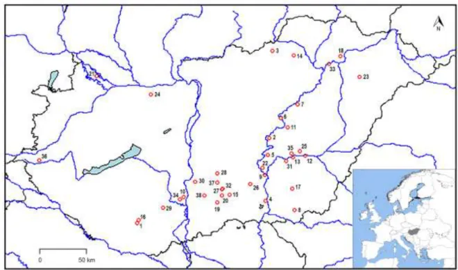
In August 2010, a total of 38 freshwater lakes were sampled in the Carpathian Basin (Fig. 2, 128
Table S2). Each of them had a surface smaller than 3 km2 and their altitude varied between 73 129
and 311 m (Table S2). Altitude of sampling sites (Table S1) were measured in Google Earth 130
Pro. The geographical distance between two sampling sites ranged from 2 to 400 km.
131
Phytobenthos samples were collected in the littoral region primarily from common 132
reed (Phragmites australis (Cav.) Trin. ex Steud.) or from other characteristic emergent 133
macrophytes, such as sedge (Carex sp.) or bulrush (Typha sp.) (CEN, 2003; King et al., 134
2006). In each case, five macrophyte stems of the same species were chosen and starting ca. at 135
10 cm below the water surface, their 15-cm sections were cut. In some lakes, where 136
7 macrophyte vegetation was not characteristic or was absent, benthic diatoms were taken from 137
permanently-submerged natural stones, boughs or in case of their absence, from mud surface 138
with pipette. In each lake, only one type of substrates was sampled. Diatom valves were 139
cleaned by hot hydrogen-peroxide method and embedded in Zrax© resin (CEN, 2003).
140
Species were identified at 1000× magnification using Zeiss Axio Imager A1 with 141
Planapochromat DIC lense (Zeiss, 518N) according to the standard taxonomic guides (Bey &
142
Ector, 2010; Hofmann et al., 2011; Krammer, 2000, 2002, 2003; Krammer & Lange-Bertalot, 143
1991, 1999a, b, 2000; Lange-Bertalot, 2001; Lange-Bertalot et al., 2011; Levkov, 2009;
144
Levkov et al., 2013). In each sample, a minimum of 400 diatom valves was counted. All 145
diatom taxa (identified at species or genera level) were regarded as individual species and 146
were included in each subsequent statistical analysis.
147
Furthermore, water physical and chemical characteristics were determined for each 148
sampling site. Water temperature, oxygen saturation (DO%), conductivity, pH and turbidity 149
were measured in situ using an HQ40d Hach Lange multimeter. In laboratory, concentration 150
of HCO3-
, Cl-, SO42-
and COD were determined titrimetrically (APHA, 1998), whereas NO2-
151 ,
NO3-, NH4+, SRP, TP (APHA 1998) and SRSi (Wetzel & Likens, 2000) 152
spectrophotometrically.
153 154
Statistical analyses 155
Prior to the metacommunity-analyses, non-metric multidimensional scaling (NMDS) was 156
performed to visualize whether community composition of benthic diatoms was separated 157
according to the substrate types. NMDS was conducted based on the Hellinger-transformed 158
species abundance data applying Bray-Curtis distance. The NMDS projection displayed that 159
benthic diatom communities were not separated according to the substrate types and their 160
8 distribution was relatively homogeneous (Fig. S1). Therefore, all samples were included in 161
the subsequent statistical analyses.
162
The relative contribution of pure and shared effect of environmental heterogeneity and 163
spatial distance to variability of diatom communities was investigated with variation 164
partitioning method (Peres-Neto et al., 2006). In this analysis, two data matrices were used to 165
define the two explanatory variable groups. One of that was the group “environmental 166
heterogeneity”, which consisted of the first two principal components’ scores produced by a 167
principal component analysis (PCA) on a correlation matrix of standardized physical and 168
chemical parameters. In the group ‘spatial distance’, distance-based Moran’s eigenvectors 169
(dbMEMs) were included as explanatory variables computed by principal coordinate analysis 170
(PCoA) of a truncated geographic distance matrix among sampling locations (Borcard &
171
Legendre, 2002; Borcard et al., 2004). Variation partitioning was performed both for 172
Hellinger transformed species abundance (Legendre & Gallagher, 2001; Borcard et al., 2011) 173
and species incidence data. ANOVA (permutations = 999) of RDA models were run to assess 174
the significance of adjusted R2 values for testable fractions (pure environmental heterogeneity 175
and spatial distance).
176
To estimate overall β-diversity of diatom communities across the 38 sampling sites, 177
first we calculated abundance-based multiple-site Bray-Curtis dissimilarity (βBC), which was 178
partitioned into its two components: abundance balanced variation (βBC.BAL) and abundance 179
gradients (βBC.GRA) (Baselga, 2017). Then, we transformed diatom abundance data into 180
presence-absence data and performed the same estimation using incidence-based multiple-site 181
Sørensen dissimilarity index (Baselga, 2010). Sørensen index (βSOR) was also divided into its 182
components: turnover (βSIM) and nestedness resultant (βNES) component (Baselga et al., 2007;
183
Baselga, 2010).
184
9 Local contribution to β-diversity was calculated for each sampling site to quantify 185
their ecological uniqueness. The computation was carried out both for abundance 186
(LCBDD%diff) and presence-absence (LCBDDS) data based on indices from the Baselga-family, 187
Sørensen group. We used percentage different dissimilarity (D%diff) for quantitative (Baselga, 188
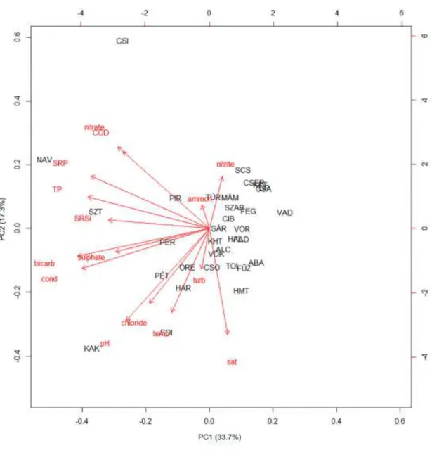
2013) and Sørensen dissimilarity (DS) for binary data (Baselga, 2010). To stratify Euclidean 189
property, we applied square-root transformation for dissimilarity matrices (D%diff and DS) 190
(Legendre & De Cáceres, 2013). To assess how unique each site is in terms of species 191
replacement and nestedness, LCBD values were computed for replacement (LCBDReplB%diff, 192
LCBDReplBS) and nestedness (LCBDNesB%diff, LCBDNesBS) decomposing LCBDD%diff and 193
LCBDDS (Legendre & De Cáceres, 2013).
194
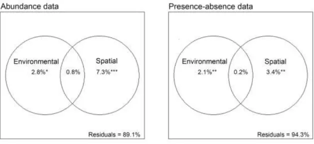
To describe the relative importance of individual species in affecting overall β- 195
diversity, we calculated species contribution to β-diversity for Hellinger-transformed 196
abundance data (SCBDab) and for species incidence data (SCBDpa) (Legendre & De Cáceres, 197
2013).
198
Since LCBD and SCBD indices (response variables) exhibit relative contribution data 199
taking values between 0 and 1, generalized additive models (GAMs) using beta regression 200
family with logit link function (Wood et al., 2016) were applied to investigate the relationship 201
of LCBDD%diff, and LCBDDS with the local species richness as well as the relationship of 202
SCBDab and SCBDpa with the number of sites occupied by a given species and with the total 203
abundance of the species. We run regression tree model analyses (Breiman et al., 1984) to 204
find the most important environmental factors determining the variation in LCBD indices 205
(LCBDD%diff, LCBDDS, LCBDReplB%diff, LCBDReplBS, LCBDReplB%diff, LCBDReplBS).
206
Furthermore, Pearson correlation coefficient was computed for each pair of LCBD indices to 207
estimate the correlation between them.
208
10 R statistical software (R. 3.4.1; R Development Core Team, 2017) was used to 209
conduct statistical analyses. We applied codep (Guenard et al., 2017) and ape (Paradis et al., 210
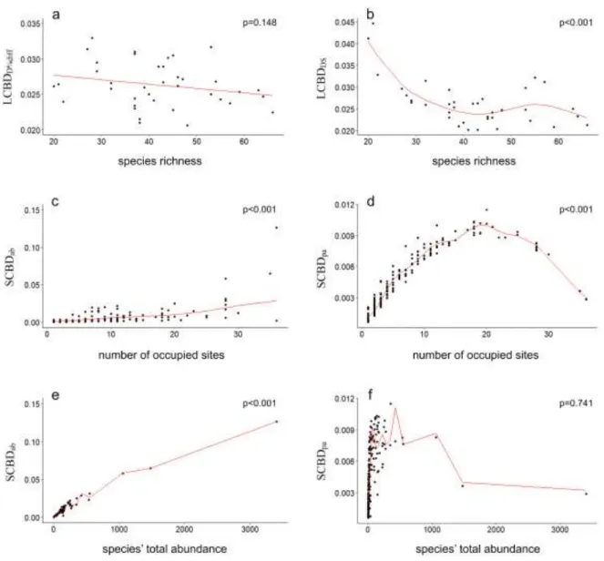
2004) R packages for dbMEM analysis and PCoA, and vegan (Oksanen et al., 2017) for 211
variation partitioning. Multiple-site β-diversity indices were calculated in betapart (Baselga et 212
al., 2017), LCBD and SCBD indices in adespatial (Dray et al., 2017), ade4 (Dray & Dufour, 213
2007) R packages and with beta.div function (Legendre & De Cáceres, 2013). Regression tree 214
model analyses and GAMs were conducted and illustrated using rpart (Therneau et al., 2017), 215
rpart.plot (Milborrow, 2017), mgcv (Wood, 2011) and ggplot2 (Wickham, 2009) R packages.
216 217
Results 218
Physical and chemical parameters varied considerably among the 38 lakes, many of them had 219
a higher standard deviation than the mean (Table S1). According to the PCA results (Fig. 3), 220
33.7% of the variance in environmental factors is explained by PC1 axis and 17.3% by PC2 221
axis. In descending order, HCO3-, conductivity, TP and SRP showed the highest correlation 222
with PC1 axis (absolute values of Pearson correlation coefficients were above 0.8) and had 223
the highest PC1 loading. Variables correlated most with PC2 axis (absolute values of Pearson 224
correlation coefficients were above 0.6) and possessing the highest PC2 loading were O2
225
saturation and pH.
226
Based on the results of variation partitioning (Fig. 4), the establishment of diatom 227
community composition was affected significantly by environmental heterogeneity and spatial 228
distance among the sampling sites as well. However, either in case of species abundance or 229
incidence data, the pure spatial distance explained a slightly higher proportion (7.3% and 230
3.4%) of community variation than environmental heterogeneity alone (2.8% and 2.1%).
231
In the 38 phytobenthos samples, 273 diatom taxa were found, of which 269 were 232
identified at species level and four at genus level. The number of species showed high 233
11 variability: its lowest value was 20 and the highest was 66 (average and standard deviation: 42 234
± 12). We found high overall β-diversity of diatom communities according to the abundance- 235
based (βBC=0.956) as well as the incidence-based (βSOR=0.934) multiple-site framework. In 236
both cases, β-diversity patterns were enhanced mainly by the component accounting for 237
species substitution (abundance balanced variation: βBC.BAL=0.953 and turnover: βSIM=0.914) 238
whereas the component accounting for subsets (abundance gradients: βBC.GRA=0.003 and 239
nestedness βNES=0.020) was very low.
240
We found strong positive correlation between LCBDD%diff and LCBDReplB%diff as well 241
as between LCBDDS and LCBDReplBS (Pearson correlation coefficients were 0.98 and 0.94, 242
respectively) furthermore, LCBDNesB%diff correlated negatively with LCBDD%diff and 243
LCBDReplB%diff (Pearson correlation coefficients were -0.51 and -0.47, respectively). For any 244
other pairs of indices, no significant correlation was displayed (Table S3). GAMs and 245
regression tree model analyses revealed that distinct factors affect the LCBD indices using 246
abundance and incidence data. There was no significant relationship between LCBDD%diff and 247
local species richness, but LCBDDS showed a significant decrease with the increase of species 248
richness (Table 1, Fig. 5a-b).
249
Sites with the highest local contribution to β-diversity were different when conducting 250
computations on species abundance and presence-absence matrix. These two types of data 251
revealed different results also during the investigation of sampling sites’ uniqueness in terms 252
of species replacement and nestedness. Sites possessing the highest LCBDD%diff index 253
(>0.030) were CSA, CSI, HAR, ÖRE and SZT (Fig. S2a), and according to the regression tree 254
model analyses, environmental variables driving LCBDD%diff were TP and NO3-
(Fig. 6a).
255
Similarly, sampling sites with the highest LCBDReplB%diff value (>0.034) were CSA, CSI, 256
HAR, ÖRE and SZT (Fig. S2b) where SRP and COD were the most decisive (Fig. 6b). In 257
turn, sites represented by the highest LCBDNesB%diff (>0.115) were KHT, TDO, VDK and 258
12 MÁM (Fig. S2c) determined primarily by TP, COD and pH (Fig. 6c). In case of the 259
incidence-based data, the highest LCBDDS indices (>0.031) were found at sites HÁM, KEN, 260
KFT, SÁR, VAD and PIR (Fig. S3a), where SRP, COD and SRSi had the most important 261
effect (Fig. 7a). HÁM, KEN, KFT, SÁR and VAD (Fig. S3b) achieved the highest 262
LCBDReplBS value (>0.036) affected mainly by SRP and NH4+
(Fig. 7b). Sites with 263
outstanding LCBDNesBS index (>0.095) were PIR, TÚR and TOL (Fig. S3c) driven by SRP 264
and TP concentration (Fig. 7c).
265
Contribution of the individual species to β-diversity depended on the type of the 266
applied data matrix (abundance- or incidence-based). According to the GAMs’ results, SCBD 267
using abundance data (SCBDab) depended both on the number of sites occupied by the given 268
species and on the total abundance of the species (Table 1, Fig. 5c, e): it showed an increasing 269
trend with the increase of both explanatory variables. In turn, SCBD based on incidence data 270
(SCBDpa) was significantly related only to the number of occupied sites and a unimodal 271
(hump-shaped) relationship was revealed between them (Table 1, Fig. 5d, f): SCBDpa 272
increased up to 20 occupied sites and then, it started to decrease. Species with the highest 273
SCBDab value (>0.05) were Achnanthidium minutissimum (Kützing) Czarnecki, Amphora 274
pediculus (Kützing) Grunow and Cocconeis placentula Ehrenberg, all of which occupied high 275
number of samples (≥28) and were present with high total abundance (≥1060 individuals 276
counted during the study). In contrast, Eolimna minima (Grunow) Lange-Bertalot, 277
Halamphora veneta (Kützing) Levkov, Nitzschia palea var. tenuirostris Grunow, Nitzschia 278
palea var. debilis (Kützing) Grunow and Nitzschia supralitorea Lange-Bertalot had the 279
highest SCBDpa (>0.01). These species occurred at intermediate proportion of sites (at 18-20 280
sites) and with moderate total abundance (110-354 individuals).
281 282
Discussion 283
13 Structuring drivers and β-diversity of diatom communities
284
In accordance with our first hypothesis, the composition of benthic diatom communities in the 285
studied small, freshwater lakes of the Carpathian Basin depended significantly on the spatial 286
variables, however, the filtering effect of the lakes’ local environmental characteristics played 287
also a significant role. Studies using variation partitioning to unravel metacommunity 288
mechanisms assume, in general, i) species-sorting if solely the “environmental variables”
289
fraction explains significantly the community structures; ii) neutral theory or patch dynamics 290
if only the “spatial variables” fraction is significant and iii) mass-effect concept or the 291
combination of species-sorting and mass-effect if both fractions have significant explanatory 292
power (Cottenie, 2005; Soininen, 2014). However, instead of regarding metacommunity 293
concepts as distinct alternatives, considering them as continuum is suggested (Alonso et al., 294
2006; Gravel et al., 2006; Leibold & McPeek, 2006; Adler et al., 2007; Chase, 2007). It is 295
impossible to firmly determine the boundaries between the types of metacommunities due to 296
several interfering factors (Leibold & Chase, 2017). The degree of environmental 297
heterogeneity within the studied area and the traits of species, such as size and dispersal rate, 298
greatly influence the response of species to habitat heterogeneity. Relatively large species 299
with low dispersal rates are assumed to be structured according to spatial variables due to 300
their limited dispersion complying with the neutral theory and patch dynamics rather than by 301
environmental characteristics. In contrast, smaller species with better dispersion abilities are 302
likely driven by habitat heterogeneity because they might be able to respond more sensitively 303
even to the minor environmental differences (Hájek et al., 2011; De Bie et al., 2012; Heino, 304
2013). In case of intermediate dispersal rates, dispersion limitation is not probable and 305
environmental heterogeneity inherent to species-sorting mechanisms is the most decisive, 306
whereas structure of the best dispersing species is slightly better explained by the spatial 307
variables and habitat heterogeneity is less important that is, mass-effect will become prevalent 308
14 (Leibold & Chase, 2017). Our variation partitioning results, and taking into account the small 309
size and the effective passive dispersion (Kristiansen, 1996; Finlay, 2002) of diatoms, point to 310
the fact that at intermediate spatial scale in the Carpathian Basin lake benthic diatoms were 311
assembled in conformity with the mass-effect theory. However, despite that diatoms are 312
regarded as relatively well dispersing organisms within large areas (e.g., at continental or 313
global scale), geographic separation tend to limit their ubiquitous dispersal thus showing pure 314
spatial patterns, which can be explained by the neutral theory (Heino et al., 2010).
315
Nevertheless, it would be difficult to decide exclusively for one metacommunity concept 316
without quantifying accurately the species’ dispersal rate and the strength of environmental 317
gradients within the studied region (Logue et al., 2011; Lindström & Langenheder, 2012;
318
Maloufi et al., 2016). In addition, the observed high proportion of unexplained variation 319
(residuals) probably deriving from unmeasured environmental parameters, undersampling of 320
rare species and stochastic processes should not be ignored during the interpretation of the 321
observed patterns. For instance, if an originally unmeasured variable were spatially structured, 322
the importance of the “spatial variables” fraction would increase, whereas if it were not 323
spatially structured, residuals would be higher, leading to distinct conclusions regarding 324
metacommunity theories (Leibold & Chase, 2017). Moreover, unregulated ecological drifts 325
and colonization-extinction stochasticity (predicted by the neutral theory and patch dynamics, 326
respectively) might also increase residual variation (Hubbell, 2001; Vellend, 2010, 2016;
327
Leibold & Chase, 2017).
328
We experienced a high average of local diatom species richness, which confirms 329
Mouquet & Loreau's (2003) theory that consequent on mass-effect, α-diversity should 330
increase if dispersal rate slightly increases. However, this process should result in a decreased 331
β-diversity among sites. Contrary to this, but in agreement with our expectations and previous 332
findings (Tisseuil et al., 2012; Maloufi et al., 2016; Viana et al., 2016; Soininen et al., 2018;
333
15 Szabó et al., 2018) that at mid-latitudes (like the Carpathian Basin) driving mechanisms 334
expounded above, resulted in very high β-diversity primarily due to the high degree of species 335
turnover among the sampling sites. In turn, nestedness resulted from richness differences was 336
inconsiderable based on our analyses. In the meta-analysis by Soininen et al. (2018) species 337
turnover and total β-diversity showed strong correlation as both quantify the compositional 338
dissimilarities between samples, whereas nestedness is represented with several times smaller 339
proportion (even close to zero) than turnover and it may only measure the bias caused by 340
richness differences. They also described that β-diversity and its turnover component are 341
slightly smaller near the poles, which could be explained by the more homogeneous 342
environment, less limited species dispersion (Mouquet & Loreau, 2003; Leibold et al., 2004) 343
and less pronounced biotic interactions (Willig et al., 2003; Schemske et al., 2009). Towards 344
higher latitudes, where glaciation might have played an important role in the local and 345
regional extinction and recolonization processes, the increase of nestedness was found 346
(Soininen et al., 2018). Either species abundance or presence-absence data were applied 347
during the analyses, we were able to draw the same conclusion that both the local 348
environment and the spatial distance influenced the benthic diatom assemblages and high β- 349
diversity was enhanced by species turnover. However, similarly to previous studies (Heino et 350
al., 2010; Vilmi et al., 2016; Szabó et al., 2018), the unexplained variation in community 351
structure was higher when only the incidence of diatom species was considered.
352 353
Local contribution of sampling sites to β-diversity 354
Calculation of LCBD is suitable for quantifying which sites contribute more (or less) to β- 355
diversity than the mean and thereby for evaluating the ecological uniqueness of communities 356
at each sites (Legendre & De Cáceres, 2013). Local contribution to β-diversity and local 357
contribution in terms of species replacement showed a strong positive relationship applying 358
16 either abundance- or incidence-based data. However, in case of using abundance data, LCBD 359
for nestedness decreased significantly with increasing LCBD and LCBD for replacement.
360
Accordingly, sites with highest uniqueness in terms of replacement contributed to the greatest 361
extent to total β-diversity of diatom communities, as well. This may be related to the fact that 362
in general, total β-diversity also correlates positively with its turnover component and 363
negatively with its nestedness component (Soininen et al., 2018). It is supposed that species- 364
rich sites exhibit low LCBD due to the greater chance of sharing species with other 365
communities (Maloufi et al., 2016). Nevertheless, our assumption that sites with low diatom 366
species richness have greater contribution to the regional β-diversity than sites with higher 367
richness, was only partly confirmed by the results. The declining trend in LCBD with 368
increasing local richness was observed both for abundance and presence-absence data, but the 369
relationship was significant only for species incidences. A part of former studies confirms, 370
whereas some of them contradicts our findings depending on the organisms and the habitat 371
type targeted. Applying abundance data for stream (Vilmi et al., 2017) and pond (Teittinen et 372
al., 2017) diatom communities, negative correlation between LCBD and species richness was 373
reported, however, this relationship was not evident for lake benthic diatoms (Vilmi et al., 374
2017). In case of dung beetles (Da Silva & Hernández, 2014) and stream insect assemblages 375
(Heino & Grönroos, 2017), LCBD decreased significantly with increasing local species 376
richness if calculations were conducted on presence-absence data, which is in line with our 377
findings. Consequently, we concluded that sites sustaining less diverse communities have 378
greater ecological uniqueness, however, this coherence varies among different groups of 379
organisms and ecosystems, furthermore also depends largely on the data type applied.
380
Our results revealed that local environmental variables affected sampling sites’
381
contribution to β-diversity, including its extension to replacement and nestedness, as well.
382
Although sites with highest LCBD indices were different based on abundance- and incidence- 383
17 based community data, we did not find explicit contrast in their main driving variables. Most 384
decisive factors were phosphorus forms for each LCBD index, which corroborates our 385
hypothesis, since these parameters displayed relatively high variance among the sites.
386
Additionally, nitrogen forms, pH, COD and SRSi were also crucial in evolving sites’
387
ecological uniqueness for diatom communities. These findings are not surprising, since 388
nutrient supply plays a key role in establishment of autotrophic algal assemblages and trophic 389
status is also related, for instance, to oxygen conditions and pH. Thereby, it affects indirectly 390
the physiological processes of aquatic organisms (Soininen, 2007). The above chemical 391
parameters have already been emphasized as master variables for freshwater lake diatom 392
communities in several previous studies (e.g., Hall & Smol, 1992; King et al., 2000; Lim et 393
al., 2001; Soininen, 2007). In addition, pH was found as one of the most influential variables 394
for subarctic ponds’ contribution to β-diversity of diatom communities (Teittinen et al., 2017).
395
In turn, some publications targeting β-diversity assessments reported that LCBD was not well 396
determined by local environmental characteristics, for instance, in case of stream insects 397
(Heino & Grönroos, 2017) and invertebrates (Tonkin et al., 2016).
398 399
Species contribution to β-diversity 400
With respect to species contribution to β-diversity, results published for different biota and 401
ecosystems are congruent, however, abundance- and incidence-based calculations displayed 402
fundamentally distinct patterns similarly to our findings. Gaston et al. (2006) emphasized the 403
tight link between abundance, its spatial variation and the number of occupied sites by a given 404
species, which may be related to our observations that diatom species occupying a high 405
number of lakes and represented by high abundance contributed the most to overall β- 406
diversity. That is, contrary to our hypothesis, common diatom species such as Achnanthidium 407
minutissimum, Amphora pediculus and Cocconeis placentula with extensive ecological 408
18 amplitude (Hofmann et al., 2011) and variable abundance at different sites exerted the greatest 409
impact on β-diversity. This pattern prevailed only in case of abundance-based SCBD similarly 410
to observations by Heino & Grönroos (2017) for stream insects and by Vilmi et al. (2017) for 411
stream and lake diatom communities. Our incidence-based calculations revealed that species 412
with intermediate occupancy had the largest contribution to β-diversity, which was also 413
observed by Heino & Grönroos (2017). This may be due to the fact that occupancy of these 414
species can vary largely across the sites (Gaston et al., 2006). Species with the highest 415
incidence-based SCBD were Eolimna minima, Halamphora veneta, Nitzschia palea var.
416
tenuirostris, N. palea var. debilis and N. supralitorea, which are relatively common and 417
possess intermediate-sized niches (Hofmann et al., 2011). Also, their total abundance was 418
intermediate in our data set but in this case, the relationship between SCBD and species’
419
abundance was statistically not significant. However, it is important to note that both 420
dependent (SCBD index) and explanatory variables (occupancy and species’ total abundance) 421
of the models are not independent mathematically, since each of them is conducted from the 422
same raw community data (even abundance or presence-absence), which might have affected 423
the strong relationship between them (Legendre & De Cáceres, 2013; Heino & Grönroos, 424
2017).
425 426
Conclusions 427
At intermediate spatial scale (2-400 km) of a mid-latitude region, where physical and 428
chemical parameters across small freshwater lakes are relatively, but not extremely 429
heterogeneous, benthic diatoms were assembled conforming most to the mass-effect 430
metacommunity concept. However, because patterns are largely dependent on several factors 431
(such as scale of heterogeneity, environmental variables considered during the study, dispersal 432
rates, size of species pool and stochastic processes), conclusions should be drawn with 433
19 caution. The high α-diversity (average of local species richness) found in the region, is in line 434
with the mass-effect paradigm, which is, in turn, inconsistent with the high β-diversity 435
enhanced mainly by species turnover. Freshwater lakes in the Carpathian Basin with the 436
highest contribution to overall β-diversity (and with the highest ecological uniqueness in 437
terms of turnover, too) hosted a lower number of diatom species than the average, however, 438
biodiversity conservation, in general, focuses on preserving species-rich sites. Furthermore, β- 439
diversity was related mainly to the regionally common species that have medium-sized or 440
broad niches, instead of the ecologically restricted ones. Therefore, we advocate the previous 441
suggestions made by Heino & Grönroos (2017) and Vilmi et al. (2017) that if a study aims 442
comprehensive conservation planning, a simultaneous application of LCBD and SCBD 443
indices combining with the focus on species-rich ecosystems and rare species would be 444
sufficient. Moreover, although abundance-based and incidence-based analyses led us to the 445
same conclusions regarding metacommunity concept and sites’ ecological uniqueness, they 446
displayed different patterns of SCBD. Consequently, for assessing species’ ecological 447
uniqueness during an extensive research of metacommunities, we recommend conducting the 448
analyses both on species abundance and binary data, especially in case of conservation 449
objectives.
450 451
Acknowledgements 452
We thank the colleagues of the Department of Limnology for their contribution in field 453
sampling and in laboratory work. The study was supported by the Széchenyi 2020 under the 454
EFOP-3.6.1-16-2016-00015 and the National Research Development and Innovation Office 455
(NKFIH K120595). Beáta Szabó was supported by the ÚNKP-17-3-IV-PE-5 New National 456
Excellence Program of the Ministry of Human Capacities.
457 458
20 Conflict of Interest
459
The authors declare that they have no conflict of interest.
460 461
21 References
462
Adler, P. B., J. HilleRislambers & J. M. Levine, 2007. A niche for neutrality. Ecology Letters 463
10: 95–104.
464
Alonso, D., R. S. Etienne & A. J. McKane, 2006. The merits of neutral theory. Trends in 465
Ecology and Evolution 21: 451–457.
466
APHA (American Public Health Association), 1998. Standard methods for the examination of 467
water and wastewater, 20th edition. United Book Press, Maltimore (MD).
468
Baselga, A., 2010. Partitioning the turnover and nestedness components of beta diversity.
469
Global Ecology and Biogeography 19: 134–143.
470
Baselga, A., 2013. Separating the two components of abundance-based dissimilarity: Balanced 471
changes in abundance vs. abundance gradients. Methods in Ecology and Evolution 4:
472
552–557.
473
Baselga, A., 2017. Partitioning abundance-based multiple-site dissimilarity into components:
474
balanced variation in abundance and abundance gradients. Methods in Ecology and 475
Evolution 8: 799–808.
476
Baselga, A., A. Jiménez-Valverde & G. Niccolini, 2007. A multiple-site similarity measure 477
independent of richness. Biology Letters 3: 642–645.
478
Baselga, A., D. Orme, S. Villeger, J. De Bortoli & F. Leprieur, 2017. betapart: Partitioning 479
Beta Diversity into Turnover and Nestedness Components. R package version 1.4-1.
480
https://CRAN.R-project.org/package=betapart 481
Bey, M-Y. & L. Ector, 2010. Atlas des diatomées des cours d’eau de la région Rhône-Alpes, 482
Tome 1-6. Direction régionale de l’Environnement, de l’Aménagement et du Logement 483
Rhône-Alpes, Lyon.
484
Borcard, D. & P. Legendre, 2002. All-scale spatial analysis of ecological data by means of 485
principal coordinates of neighbour matrices. Ecological Modelling 153: 51–68.
486
22 Borcard, D., F. Gillet & P. Legendre, 2011. Numerical Ecology with R. Springer, New York.
487
Borcard, D., P. Legendre, C. Avois-Jacquet & H. Tuomisto, 2004. Dissecting the spatial 488
structure of ecological data at multiple scales. Ecology 85: 1826–1832.
489
Breiman, L., J. H. Friedman, R. A. Olshen & C. J. Stone, 1984. Classification and Regression 490
Trees. Wadsworth International Group, Belmont.
491
CEN (Comité Européen de Normalisation), 2003. Water Quality Guidance Standard for the 492
Routine Sampling and Pretreatment of Benthic Diatoms from Rivers. EN 13946:2003, 493
Geneva.
494
Chase, J. M., 2007. Drought mediates the importance of stochastic community assembly.
495
Proceedings of the National Academy of Sciences 104: 17430–17434.
496
Conradi, T., V. M. Temperton & J. Kollmann, 2017. Beta diversity of plant species in human- 497
transformed landscapes: Control of community assembly by regional productivity and 498
historical connectivity. Perspectives in Plant Ecology, Evolution and Systematics 24: 1–
499
500 10.
Cottenie, K., 2005. Integrating environmental and spatial processes in ecological community 501
dynamics. Ecology Letters 8: 1175–1182.
502
Da Silva, P. G. & M. I. M. Hernández, 2014. Local and regional effects on community 503
structure of dung beetles in a mainland-island scenario. PLoS One 9: e111883.
504
De Bie, T., L. De Meester, L. Brendonck, K. Martens, B. Goddeeris, D. Ercken, H. Hampel, L.
505
Denys, L. Vanhecke, K. Van der Gucht, J. Van Wichelen, W. Vyverman & S. A. J.
506
Declerck, 2012. Body size and dispersal mode as key traits determining metacommunity 507
structure of aquatic organisms. Ecology Letters 15: 740–747.
508
Dong, X., B. Li, F. He, Y. Gu, M. Sun, H. Zhang, L. Tan, W. Xiao, S. Liu & Q. Cai, 2016.
509
Flow directionality, mountain barriers and functional traits determine diatom 510
metacommunity structuring of high mountain streams. Scientific Reports 6: 24711.
511
23 Dray, S. & A. B. Dufour, 2007. The ade4 package: implementing the duality diagram for 512
ecologists. Journal of Statistical Software. 22: 1–20.
513
Dray, S., G. Blanchet, D. Borcard, G. Guenard, T. Jombart, G. Larocque, P. Legendre, N.
514
Madi & H. H. Wagner, 2017. adespatial: Multivariate Multiscale Spatial Analysis. R 515
package version 0.0-8. https://CRAN.R-project.org/package=adespatial 516
Finlay, B. J., 2002. Global dispersal of free-living microbial eukaryote species. Science 296:
517
1061–1063.
518
Gaston, K. J., P. A. V. Borges, F. He & C. Gaspar, 2006. Abundance, spatial variance and 519
occupancy: Arthropod species distribution in the Azores. Journal of Animal Ecology 75:
520
646–656.
521
Göthe, E., D. G. Angeler, S. Gottschalk, S. Löfgren & L. Sandin, 2013. The influence of 522
environmental, biotic and spatial factors on diatom metacommunity structure in Swedish 523
headwater streams. PLoS One 8: e72237.
524
Gravel, D., C. D. Canham, M. Beaudet & C. Messier, 2006. Reconciling niche and neutrality:
525
The continuum hypothesis. Ecology Letters 9: 399–409.
526
Guenard, G., P. Legendre & with contributions from B. Pages, 2017. codep: Multiscale 527
Codependence Analysis. R package version 0.6-5. https://CRAN.R- 528
project.org/package=codep 529
Hájekm, M., J. Roleček, K. Cottenie, K. Kintrová, M. Horsák, A. Poulíčková, P. Hájková, M.
530
Fránková & D. Dítě, 2011. Environmental and spatial controls of biotic assemblages in a 531
discrete semi-terrestrial habitat: Comparison of organisms with different dispersal 532
abilities sampled in the same plots. Journal of Biogeography 38: 1683–1693.
533
Hall, R. I. & J. P. Smol, 1992. A weighted—averaging regression and calibration model for 534
inferring total phosphorus concentration from diatoms in British Columbia (Canada) 535
lakes. Freshwater Biology 27: 417–434.
536
24 Heino, J., 2013. Environmental heterogeneity, dispersal mode, and co-occurrence in stream 537
macroinvertebrates. Ecology and Evolution 3: 344–355.
538
Heino, J., L. M. Bini, S. M. Karjalainen, H. Mykrä, J. Soininen, L. C. G. Vieira & J. A. F.
539
Diniz-Filho, 2010. Geographical patterns of micro-organismal community structure: Are 540
diatoms ubiquitously distributed across boreal streams? Oikos 119: 129–137.
541
Heino, J. & M. Grönroos, 2017. Exploring species and site contributions to beta diversity in 542
stream insect assemblages. Oecologia 183: 151–160.
543
Hofmann, G., M. Werum & H. Lange-Bertalot, 2011. Diatomeen im Süßwasser- Benthos von 544
Mitteleuropa. Koeltz Scientific Books, Königstein.
545
Hubbell, S. P., 2001. The Unified Neutral Theory of Biodiversity and Biogeography.
546
Princeton University Press, Princeton, New Jersey.
547
King, L., P. Barker & R. I. Jones, 2000. Epilithic algal communities and their relationship to 548
environmental variables in lakes of the English Lake District. Freshwater Biology 45:
549
425–442.
550
King, L., G. Clarke, H. Bennion, M. Kelly & M. Yallop, 2006. Recommendations for 551
sampling littoral diatoms in lakes for ecological status assessments. Journal of Applied 552
Phycology 18: 15–25.
553
Krammer, K., 2000. Diatoms of Europe: Diatoms of the European Inland Waters and 554
Comparable Habitats (Vol. 1. The Genus Pinnularia). ARG Gantner Verlag KG, Ruggel.
555
Krammer, K., 2002. Diatoms of Europe: Diatoms of the European Inland Waters and 556
Comparable Habitats (Vol. 3. Cymbella). ARG Gantner Verlag KG, Ruggel.
557
Krammer, K., 2003. Diatoms of Europe: Diatoms of the European Inland Waters and 558
Comparable Habitats (Vol. 4. Cymbopleura, Delicata, Navicymbula, 559
Gomphocymbellopsis, Afrocymbella). ARG Gantner Verlag KG, Ruggel.
560
25 Krammer, K. & H. Lange-Bertalot, 1991. Bacillariophyceae 4. Teil: Achnanthaceae. Kritische 561
Ergänzungen zu Navicula (Lineolatae) und Gomphonema. In Ettl, H., J. Gerloff, H.
562
Heynig & D. Mollenhauer D (eds), Süsswasserflora von Mitteleuropa, Band 2/4.
563
Spektrum Akademischer Verlag, Heidelberg.
564
Krammer, K. & H. Lange-Bertalot, 1999a. Bacillariophyceae 1. Teil: Naviculaceae. In Ettl, 565
H., J. Gerloff, H. Heynig & D. Mollenhauer D (eds), Süsswasserflora von Mitteleuropa, 566
Band 2/1. Spektrum Akademischer Verlag, Heidelberg.
567
Krammer, K. & H. Lange-Bertalot, 1999b. Bacillariophyceae 2. Teil: Bacillariaceae, 568
Epithemiaceae, Surirellaceae. In Ettl, H., J. Gerloff, H. Heynig & D. Mollenhauer D 569
(eds), Süsswasserflora von Mitteleuropa, Band 2/2. Spektrum Akademischer Verlag, 570
Heidelberg.
571
Krammer, K. & H. Lange-Bertalot, 2000. Bacillariophyceae 3. Teil: Centrales, Fragilariaceae, 572
Eunotiaceae. In Ettl, H., J. Gerloff, H. Heynig & D. Mollenhauer D (eds), 573
Süsswasserflora von Mitteleuropa, Band 2/3, Spektrum Akademischer Verlag, 574
Heidelberg.
575
Kristiansen, J., 1996. Dispersal of freshwater algae — a review. Hydrobiologia 336: 151–157.
576
Lange-Bertalot, H., 2001. Diatoms of Europe Diatoms of the European Inland Waters and 577
Comparable Habitats (Vol. 2. Navicula sensu stricto. 10 genera separated from Navicula 578
sensu lato. Frustulia). ARG Gantner Verlag KG, Ruggel.
579
Lange-Bertalot, H., M. Malgorzata & A. Witkowski, 2011. Diatoms of Europe: Diatoms of the 580
European Inland Waters and Comparable Habitats (Vol. 6. Eunotia and some related 581
genera). ARG Gantner Verlag KG, Ruggel.
582
Langenheder, S. & H. Ragnarsson, 2007. The role of environmental and spatial factors for the 583
composition of aquatic bacterial communities. Ecology 88: 2154–2161.
584
26 Legendre, P., 2014. Interpreting the replacement and richness difference components of beta 585
diversity. Global Ecology and Biogeography 23: 1324–1334.
586
Legendre, P. & M. De Cáceres, 2013. Beta diversity as the variance of community data:
587
Dissimilarity coefficients and partitioning. Ecology Letters 16: 951–963.
588
Legendre, P. & E. D. Gallagher, 2001. Ecologically meaningful transformations for ordination 589
of species data. Oecologia 129: 271–280.
590
Leibold, M. A. & J. M. Chase, 2017 Metacommunity Ecology, Princeton University Press, 591
Princeton, New Jersey.
592
Leibold, M. A. & M. A. McPeek, 2006. Coexistence of the niche and neutral perspectives in 593
community ecology. Ecology 87: 1399–1410.
594
Leibold, M. A., M. Holyoak, N. Mouquet, P. Amarasekare, J. M. Chase, M. F. Hoopes, R. D.
595
Holt, J. B. Shurin, R. Law, D. Tilman, M. Loreau & A. Gonzales, 2004. The 596
metacommunity concept: A framework for multi-scale community ecology. Ecology 597
Letters 7: 601–613.
598
Levkov, Z., 2009. Diatoms of Europe: Diatoms of the European Inland Waters and 599
Comparable Habitats (Vol. 5. Amphora sensu lato). ARG Gantner Verlag KG, Ruggel.
600
Levkov, Z., D. Metzeltin & A. Pavlov, 2013. Diatoms of Europe: Diatoms of the European 601
Inland Waters and Comparable Habitats (Vol. 7. Luticola and Luticolopsis). Koeltz 602
Scientific Books, Königstein.
603
Lim. D. S. S., C. Kwan, M. S. V. Douglas, 2001. Periphytic diatom assemblages from Bathurst 604
Island, Nunavut, Canadian High Arctic: An examination of community relationships and 605
habitat preferences. Journal of Phycology 37: 379–392.
606
Lindström, E. S. & S. Langenheder, 2012. Local and regional factors influencing bacterial 607
community assembly. Environmental Microbiology Reports 4: 1–9.
608
27 Logue, J. B., N. Mouquet, H. Peter & H. Hillebrand, 2011. Empirical approaches to 609
metacommunities: a review and comparison with theory. Trends in Ecology and 610
Evolution 26: 482–491.
611
Lopes, P. M., L. M. Bini, S. A. J. Declerck, V. F. Farjalla, L. C. G. Vieira, C. C. Bonecker, F.
612
A. Lansac-Toha, F. A. Esteves & R. L. Bozelli, 2014. Correlates of zooplankton beta 613
diversity in tropical lake systems. PLoS One 9: e109581.
614
Maloufi, S., A. Catherine, D. Mouillot, C. Louvard, A. Couté, C. Bernard & M. Troussellier, 615
2016. Environmental heterogeneity among lakes promotes hyper β-diversity across 616
phytoplankton communities. Freshwater Biology 61: 633–645.
617
Milborrow, S., 2017. rpart.plot: Plot 'rpart' Models: An Enhanced Version of 'plot.rpart'. R 618
package version 2.1.2. https://CRAN.R-project.org/package=rpart.plot 619
Mouquet, N. & M. Loreau, 2003. Community Patterns in Source‐Sink Metacommunities. The 620
American Naturalist 162: 544–557.
621
Mykrä, H., J. Heino & T. Muotka, 2007. Scale-related patterns in the spatial and 622
environmental components of stream macroinvertebrate assemblage variation. Global 623
Ecology and Biogeography 16: 149–159.
624
Oksanen, J., F. G. Blanchet, M. Friendly, R. Kindt, P. Legendre, D. McGlinn, P. R. Minchin, 625
R. B. O’Hara, G. L. Simpson, P. Solymos, M. H. H. Stevens, E. Szoecs & H. Wagner, 626
2017. vegan: Community Ecology Package. R package version 2.4-3. https://CRAN.R- 627
project.org/package=vegan 628
Paradis, E., J. Claude & K. Strimmer, 2004. APE: analyses of phylogenetics and evolution in 629
R language. Bioinformatics 20: 289–290.
630
Peres-Neto, P. R., P. Legendre, S. Dray & D. Borcard, 2006. Variation partitioning of species 631
data matrices: Estimation and comparison of fractions. Ecology 87: 2614–2625.
632