Discrete LPV Modeling of Diabetes Mellitus for Control Purposes
Gy¨orgy Eigner∗, M´at´e Siket†, Anik´o Szak´al ‡, Imre Rudas ‡, Levente Kov´acs∗
∗Physiological Controls Research Center
Research, Innovation and Service Center, ´Obuda University, Budapest, Hungary Email:{eigner.gyorgy,kovacs.levente}@nik.uni-obuda.hu
† Budapest University of Technology and Economics, Budapest, Hungary Email: siket.mate@gmail.com
‡Research, Innovation, and Service Center, ´Obuda University, Budapest, Hungary Email:{rudas,szakal}@uni-obuda.hu
. Abstract—The utilization of modern and advanced control engineering related methods for the control, estimation and assessment of physiological applications is widespread. It is also well-known that this engineering apparatus is executed on digital computers. The current insufficiency of available and accurate discretized models, especially in case of Diabetes Mellitus (DM), provides incentive for this research. The researchers typically approximate the continuous solutions which may not be the best alternative in many cases, in particular considering numerical stability and cost-effectiveness. In this paper we performed an analysis of the available discretization options in order to develop discrete models with a special focus on the Linear Parameter Varying (LPV) systems. LPV techniques are very useful frame- works which allow the application of linear controller, observer and estimator design. In this study, three LPV discretization and two Jacobian based discretization methods are introduced and analyzed to provide a basis for our further investigations in the topic.
Index Terms—Linear Parameter Varying techniques, Dis- cretization, Discrete LPV Modeling, Diabetes Mellitus
I. INTRODUCTION
Control Engineering (CE) approaches have inevitable role regarding physiological, biological and chemical applications.
In the recent years many practical application shown that by in- volving the latest results of CE into physiological applications better performance and better management of the treatments can be achieved [1]–[7].
On the field of biomedical engineering DM receives an ever growing scientific attention due to the continuously increasing number of people who are affected. By the newest approx- imations, there are 425 million people worldwide who live with DM in 2018, this estimation involves undiagnosed cases also beside the diagnosed ones [8]. Furthermore, the current predictions imply that this number will reach 629 million, the 6.65% of the expected world population by 2045 [8].
Gy. Eigner was supported by the ´UNKP-17-4/I. New National Excellence Program of the Ministry of Human Capacities. This project has received funding from the European Research Council (ERC) under the European Union’s Horizon 2020 research and innovation programme (grant agreement No 679681)
This paper focuses on Type 1 Diabetes Mellitus (T1DM).
This is a disorder of the natural blood glucose level regulatory system. Insulin hormone plays one of the most important part in the glucose homeostasis. T1DM involves an acute autoimmune reaction, where the result is the perishing of insulin producer β-cells [9]. Insulin is the indicator for the body cells, that the blood glucose level is elevated, and it ought to facilitate the glucose molecules by making the cell membrane permeable for them. Patients in such a diabetic condition are in need of external insulin injection, because due to the osmotic pressure cells dehydrate, on the long run energetic collapse can occur. [10], [11]. The control of the blood glucose level of a diabetic patient is crucial, because the uncontrolled disease can lead to several negative effect [8]. Furthermore, the characteristics and quality of the control is also essential [12].
In case of T1DM the tight glycemic control (TGC) is the key of good glycemic status. TGC requires frequent BG measure- ments via finger pricks (manual measurement) or Continuous Glucose Monitoring System (CGMS) [13]. There are still many challenges regarding CGMS technology, however. For example, the sampling frequency is around 5 minutes on basis, noise and disturbance sensitivity, inaccuracies of available mathematical models, etc. [2], [5], [14]. State estimation for control applications is also an important aspect which is not trivial and the requirements of it determined by the type of control to be applied [15], [16]. In our previous work, we have presented the use of LPV methodology regarding the control of DM [17]–[19].
Both for LPV based state estimation and control the in- vestigation of possible discretization techniques is necessary.
Through the scaled and discretized models it is possible to taking into account all requirements coming from the estima- tors (e.g. Kalman filter), LPV controller and available sensor technology (sampling time, disturbances, etc.).
The paper is structured as follows. First, we introduce the models to be investigated. After, the discretization possibili- ties regarding the presented models are shown. Finally, our findings are described and we conclude our work.
2018 IEEE International Conference on Systems, Man, and Cybernetics
II. APPLIEDMODELS
A. The Minimal Model
We have investigated the well-known T1DM model of Bergman in the form presented by [20]. The model has three state variables: G(t) mg/dL is the blood glucose (BG) concentration, X(t) 1/min insulin-excitable tissue glucose uptake activity, I(t) U/mL blood insulin concentration. The w(t)mg/dL/min is the disturbance input (the glucose intake) andu(t)U/mL/min is the control input (insulin intake). The output of the system is the BG concentration G(t)which is measurable. Thep1,p2,p3andn, are model parameters. In this study we have applied the following data set:[p1, p2, p3, n] = [0.028,0.025,0.00013,0.23]based on [20].
G(t) =˙ −(p1+X(t))G(t) +p1GB+w(t). (1a) X(t) =˙ −p2X(t) +p3[I(t)−IB]. (1b) I(t) =˙ −n[I(t)−IB] +u(t). (1c) B. LPV Modeling in General
In the following the continuous and discrete state-space LPV (LPV-SS) model description – in a general manner – are presented.
Definition 1. Continuous-Time LPV-SS Model [21], [22].
The continuous time LPV-SS model (CT-LPV) can be described by the following differential equations (without considering separated disturbance input):
x˙c(t) =
Ac(pc(t))xc(t) +Bc(pc(t))uc(t) +Ec(pc(t))dc(t) , (2a) yc(t) =
Cc(pc(t))xc(t) +Dc(pc(t))uc(t) +D2,c(pc(t))dc(t) , (2b) whereAc(pc(t))∈Rn×n,Bc(pc(t))∈Rn×m,Ec(pc(t))∈ Rn×z, Cc(pc(t)) ∈ Rk×n, Dc(pc(t)) ∈ Rk×m and D2,c(pc(t)) ∈ Rk×z are the pc(t) dependent system-, input-, disturbance-, output-, input-coupling- and disturbance- coupling matrices, respectively and xc(t) ∈ Rn is the state vector. Theuc(t)∈Rm is the input vector, whiledc(t)∈Rz is the disturbance vector. Thepc(t) = [p1,c(t). . . pR,c(t)]pa- rameter vector consists of the so-called scheduling parameters pi,c(t).pc(t)∈ ΩR ∈ RR is an R dimensional real vector within the Ω = [p1,c,min, p1,c,max]×[p2,c,min, p2,c,max]× . . .×[pR,c,min, pR,c,max] ∈ RR hyperplane inward the RR real vector space. If any of the states is selected as scheduling variable, the given LPV model becomes a quasi-LPV (qLPV) model [21], [22].
By assuming an ideal zero-order hold (ZOH) device,pc(t), uc(t)anddc(t)are constant within each sampling interval. In this case the continuous system can be written as:
˙xc(t) =
Ac(pc(kTd))xc(t) +Bc(pc(kTd))uc(kTd)+
Ec(pc(kTd))dc(kTd) , (3a)
yc(t) =
Cc(pc(kTd)))xc(t) +Dc(pc(kTd))uc(kTd)+
D2,c(pc(kTd))dc(kTd) , (3b) wherekis the discrete step and Td is the sampling time.
Definition 2. Discrete-Time LPV-SS Model [21], [22].
The discrete time LPV-SS model (CT-LPV) can be de- scribed by the following difference equations:
xd(k+ 1) =
Ad(pd(k))xd(k) +Bd(pd(k))ud(k)+
Ed(pd(k))dd(k) , (4a) yd(k) =
Cd(pd(k))xd(k) +Dd(pd(k))ud(k)+
D2,d(pd(k))dd(k) , (4b) where the matrices and vectors are the discrete time equiva- lents of the continuous time counterparts andkis the sampling time instance.
C. Investigated LPV Model
Due to our aim is to provide appropriate discrete time LPV models for our further research, we have developed a qLPV model form of (1a)-(1c).
Because theG(t)variable is the nonlinearity causing term, we have selected it as scheduling parameter, namely,p(t) = p(t) =G(t)from (1a). This is the most straightforward way to represent the system in qLPV form.
The (1a)-(1c) contain thep1GB,−p3IBandn IBconstant terms. These are needed to be handled as ”input signals” from the qLPV system point of view. Since these are constant terms, it does not matter whether we represent them in theBor in theEmatrix. However, our aim is to apply them for controller and estimator design in the future. Hence, it is more suitable if these terms are part of theEmatrix – beside the disturbance input. Thus, thed(t) = [1 1 1w(t)].
By considering the aforementioned conditions and using the LPV principle the following qLPV state-space representation can be written:
˙
x(t) =A(p(t))x(t) +Bu(t) +Ed(t) , (5a) y(t) =Cx(t) +Du(t) +D2d(t) , (5b)
A(p(t)) =
⎡
⎣−p1 −G(t) 0 0 −p2 p3
0 0 −n
⎤
⎦,
B=
⎡
⎣0 01
⎤
⎦, E=
⎡
⎣p1GB 0 0 1
0 −p3IB 0 0
0 0 n IB 0
⎤
⎦, C=
1 0 0
, D=
0 0 0 ,
(5c)
where the constant terms are represented inE.
III. DISCRETIZATIONPROCEDURES
We intended to provide a full picture about the available discretization techniques, how they can be applied regard- ing the given cases. Hence, we investigated the ”classical”
methods as well (Jacobian based discretization), not just the LPV discretization opportunities. In this way, the comparison between them became possible.
A. Complete LPV-SS discretization
In this case, the CT-LPV system as it is described by (3) is transformed by using the LTI assumption of complete signal evolution approach sampling with ZOH [21]. The method results an approximating DT-LPV system in the form of (4) with given approximation error. The transformation is step-by- step described by (6a)–(6d) in accordance with [23], [24].
Ad(pd(k)) =e(Ac(pc(kTd))Td) , (6a) Bd(pd(k)) =
A−1c (pc(kTd)(e(Ac(pc(kTd))Td)−I)Bc(pc(kTd)) , (6b) Ed(pd(k)) =
A−1c (pc(kTd)(e(Ac(pc(kTd))Td)−I)Ec(pc(kTd)) , (6c) Cd(pd(k)) =Cc(pc(kTd)) , (6d) Dd(pd(k)) =Dc(pc(kTd)) , (6e) D2,d(pd(k)) =D2,c(pc(kTd)) . (6f) B. Rectangular LPV-SS discretization
The rectangular method can be derived from the first order forward Euler’s method [23]–[25].
Ad(pd(k)) =I+TdAc(pc(kTd)) , (7a) Bd(pd(k)) =TdBc(pc(kTd)) , (7b) Ed(pd(k)) =TdEc(pc(kTd)) , (7c) Cd(pd(k)) =Cc(pc(kTd)) , (7d) Dd(pd(k)) =Dc(pc(kTd)) , (7e) D2,d(pd(k)) =D2,c(pc(kTd)) , (7f) C. Adams-Bashforth LPV-SS discretization
From the family of multi-step methods, the Adams- Bashforth discretization can be implemented due to the ne- cessity of fixed step size. Below, the general form of the three step method given, which results in a 9th order system [23], [24], [26]:
Ad(pd(k)) =
⎡
⎣I+23T12dAc(pc(kTd)) −16T12dI 5T12dI Ac(pc(kTd)) 0 0
0 I 0
⎤
⎦ , (8a)
Bd(pd(k)) = 23T
12dBc(pc(kTd)) Bc(pc(kTd)) 0 , (8b)
Ed(pd(k)) = 23T
12dEc(pc(kTd)) Ec(pc(kTd)) 0 , (8c) Cd(pd(k)) =
Cc(pc(kTd)) 0 0
, (8d)
Dd(pd(k)) =Dc(pc(kTd)) , (8e) D2,d(pd(k)) =D2,c(pc(kTd)) , (8f) xd(k) =
xd f|(k−1)Td f|(k−2)Td . (8g) where xd is the altered state matrix, in which the f vectors corresponds to the original continuous system equations.
D. Complete Jacobian Linearized-SS Discretization
With the Jacobian-matrix, a linear approximation has been acquired around the current step, and the system discretized by the complete method mentioned before (6a)–(6d) [23], [24].
Ad(k) =e(Aj(kTd))Td) , (9a) Bd(k) =A−1j (kTd)(e(Aj(kTd)Td)−I)Bj(kTd) , (9b) Ed(k) =A−1j (kTd)(e(Aj(kTd)Td)−I)Ej(kTd) , (9c) Cd(k) =Cj(kTd) , (9d) Dd(k) =Dj(kTd) , (9e) D2,d(k) =D2,j(kTd) , (9f) whereAj(kTd),Bj(kTd),Ej(kTd),Cj(kTd),Dj(kTd)and D2,j(kTd)are the Jacobian form of the above defined matri- ces.
E. Jacobian Linearized Recursive Discretization
In this method the state matrices are not specified, because they were calculated according to the complete method (6a)–
(6d) given in [23], [24]. The current values are calculated in each time step from the initial values, by calculating the total effect of the inputs up to the given point.
xd(k) = Ad(k)kx(0) +k−1
i=0
Ad(k)k−i−1
Bd(k)ud(i)+
Ed(k)dd(i) , (10a)
yd(k) =Cdxd(k) +Ddud(k) +D2,ddd(k). (10b)
IV. RESULTS
In this paper we do not aim to characterize the discretization error caused by the LPV discretization procedures in Sec. III.
We have investigated only the applicability of them in case of the given highly non-linear and rapidly varying glucose- insulin model. The further investigation in this regard will be the part of our future work.
It should be noted that we have used the MATLAB 2017b environment for the developments.
In order to validate the discretized systems we have applied the inbuiltode45()function of the MATLAB [27] in which we realized the original model described by Eqs. 1a-1c. This sys- tem was applied as reference system during the investigations to which all of the developed discretized systems have been compared. The ode45() is a suitable nonstiff solver solving nonlinear ordinary differential equations (ODEs) on a variable basis [27].
Since the investigated DM model has impulse like inputs, the functions had to be solved for every minutes indepen- dently. This results a quasi discrete reference model. The quantitative comparisons have been made by applying 2-norm error between the state variables of the system in all cases, namely, xODE45(t)−xDiscretized Systems(kT), where the xDiscretized Systems(kT) were the realized DT-LPV sys- tems (LPVComplete, LPVRectangular, LPVAdams−Bashf orth, LPVComplete) and the DT-SS systems based on Jacobians (Jacobian Linearized-SS and Jacobian Linearized Recursive Discretization). The states of the discretized systems were hold for the appliedT in each step in order to approximate the orig- inal continous system. As we compared all of the discretized systems to the reference system we got a picture about how the discretized systems related to each other indirectly.
The following initial values have been applied: x(t0) = [G(0), X(0), I(0)]= [115,0,15].
For testing purposes a realistic manual glucose and insulin administration scheme have been developed [28]. The glucose input consists of 500 g carbohydrate, divided into five smaller boluses. The insulin injections introduced with a five minute delay. Therefore, the inputs defined as follows: w(ti) = [65,25,75,25,60] g in each ti = [30,250,500,800,1200]
min and u(tj) = [15,5,17,5,14] mU/min in each tj = [35,255,505,805,1205] min.
The basal levels of the three state variable have been chosen to be: xB = [GB, XB, IB] = [85,0,15]. From physiological point of view basal levels correspond to the fasting conditions, from mathematical point of view the basal levels are the equilibrium points of the isolated system [29], [30].
Sampling time T was chosen to be T = 5 min due to the current blood glucose concentration measuring devices are capable of providing data at similar frequencies [5], [13] – with one exception. During our investigations it became clear that the Adams-Bashforth method was not able to provide acceptable outcome with T = 5. In accordance with our examinations we appliedT = 2min as the highest sampling
time in this case. Thus, it’s practical applicability strongly depends on the available sensor technology.
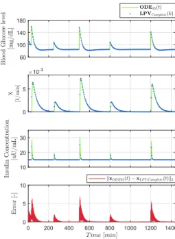
Figure 1 shows the result of the simulation of the reference and discretized systems by using the complete LPV-SS dis- cretization in accordance with III-A. It is clearly visible that the Complete LPV-SS model is able to approach the reference system with good accuracy. The norm based error shows that higher difference occurs when the systems changing due to the intakes. However, the state errors decay fast.
Figure 1. Comparison of the reference and complete DT-LPV systems.
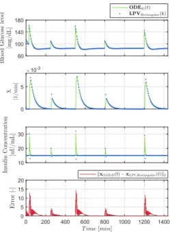
Figure 2 presents the comparison of the rectangular DT-LPV system (III-B) and the original system during operation. The results are similar to the previous case. The amplitude of the state errors are bigger, however, they decay faster compared to the complete DT-LPV model. We have found that the state error – in general – increased rapidly by usingT >5minutes, thus the use of higher sampling time is not recommended. The potential instability can be seen on Fig. 2 as well. After the injection of each bolus, the insulin concentration deviated in negative direction.
Figure 3 shows the comparison of the DT-LPV system provided by the Adams-Bashforth method (III-C) and the original system during operation. That was the only method in which we have not been able to apply the determined T = 5 sampling time (instead T = 2 was used) – as we mentioned above. It is clearly visible that this method provided the highest state errors and its inaccuracy was at the border of acceptability. As we found, the method is not able to handle the fast changes (around the intakes) at all. However, in case of ”slower” systems it may be applicable. We could not apply T >5due to instability.
Figure 2. Comparison of the reference and the rectangular DT-LPV models.
Figure 3. Comparison of the reference model and the DT-LPV model provided by the Adams-Basforth LPV-SS discretization.
Figure 4 shows the comparison of the discrete system (according to III-D) and the original system during operation.
It can be seen that the highest state error is at theG(t)due to the nonlinearity – other states of the reference system are approached by the discrete system with good accuracy. We have found, that the stability of this opportunity is good and evenT = 10can be applied without critical issues in accuracy
and numerical stability.
Figure 4. Comparison of the reference model and the discretized model (by using Jacobian linearization and complete discretization).
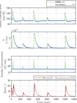
Figure 5 shows the comparison of the discrete system provided by the Jacobian recursive method (III-E) and the original system during operation. The key difference between the recursive and the complete method is that in case of the recursive method the states are calculated from the initial values in each step. The accuracy of the discrete model is similar as in the previous case – the reasons are similar as well. Although, the state errors are bigger in general and the discrete model provided unexpected behavior at the beginning of the simulations (initial deviations).
The numerical assessment can be found in Table I, where the Root Mean Square Errors (RMSE) based metric [31] has been applied to assess the quantitative differences between the systems during operation.
Table I RMSEERRORS
Systems RMSEG RMSEX RMSEI
ODE45/Complete 0.739 1.722 0.327
ODE45/Rectangular 1.321 5.676 0.921 ODE45/Adams-Bashforth 6.167 7.141 1.560 ODE45/Jacobian, Complete 4.292 1.722 0.327 ODE45/Jacobian, Recursive 5.065 2.042 0.384
As it can be seen both in the Figs 1–5 and in Table I the complete method provided the most accurate results both in case of the LPV and the Jacobian based cases. Hence, the use of this method is recommended in the further researches as a basis to design discrete LPV controllers or discrete estimators (eg. Kalman filter).
Figure 5. Comparison of the reference model and the discretized model (by using Jacobian linearization and recursive discretization).
V. CONCLUSION ANDFURTHERWORK
In this paper we have analyzed the discretization opportu- nities of a well-known DM model with a special focus on the LPV (qlPV) techniques.
We have found that the best DT-LPV model and discrete Jacobian based models have been provided by the complete method – which were proven by the RMSE based error assessment as well.
In our future work we will use the developed DT-LPV model (provided by the complete LPV-SS discretization algo- rithm) to develop DT-LPV controllers and advanced Kalman- filters (e.g. extended or unscented Kalman-filter on LPV basis).
ACKNOWLEDGMENT
The Authors thankfully acknowledge the support of the Robotics Special College of ´Obuda University and the ´Obuda University’s Research, Innovation and Service Center.
REFERENCES
[1] D. Copot, R. De Keyser, J. Juchem, and C. Ionescu, “Fractional order impedance model to estimate glucose concentration: in vitro analysis,”
ACTA Pol Hung, vol. 14, no. 1, pp. 207–220, 2017.
[2] L. M. Huyett, E. Dassau, H. C. Zisser, and F. J. Doyle III, “Glucose Sensor Dynamics and the Artificial Pancreas: The Impact of Lag on Sensor Measurement and Controller Performance,” IEEE Contr Syst, vol. 38, no. 1, pp. 30–46, 2018.
[3] M. Messori, G. P. Incremona, C. Cobelli, and L. Magni, “Individualized model predictive control for the artificial pancreas: In silico evaluation of closed-loop glucose control,”IEEE Contr Syst, vol. 38, no. 1, pp.
86–104, 2018.
[4] B. W. Bequette, F. Cameron, B. A. Buckingham, D. M. Maahs, and J. Lum, “Overnight Hypoglycemia and Hyperglycemia Mitigation for Individuals with Type 1 Diabetes: How Risks Can Be Reduced,”IEEE Contr Syst, vol. 38, no. 1, pp. 125–134, 2018.
[5] R. Nimri, A. Murray, N. abd Ochs, J. Pinsker, and E. Dassau, “Closing the Loop,”Diabetes Technol The, vol. 19, no. 1, pp. s27 – s41, 2017.
[6] D. Drexler, J. S´api, and L. Kov´acs, “Modeling of tumor growth incorpo- rating the effects of necrosis and the effect of bevacizumab,”Complexity, vol. 2017, 2017.
[7] J. S´api, D. A. Drexler, and L. Kov´acs, “Potential benefits of discrete- time controllerbased treatments over protocol-based cancer therapies,”
Acta Polytechnica Hungarica, vol. 14, no. 1, pp. 11–23, 2017.
[8] International Diabetes Federation,IDF Diabetes Atlas, 8th ed. Brussel, Belgium: International Diabetes Federation, 2017.
[9] R. DeFronzo, E. Ferrannini, P. Zimmet, and G. Alberti,International Textbook of Diabetes Mellitus, 2 Volume Set, 4th ed. Wiley-Blackwell, 2015.
[10] American Diabetes Association, “Diagnosis and classification of dia- betes mellitus,”Diab Care, vol. 37, no. Supplement 1, pp. S81–S90, 2014.
[11] W. Boron and E. Boulpaep,Medical Physiology, 3rd ed. Heidelberg, Germany: Elsevier, 2016.
[12] T. Ferenci, A. K¨orner, and L. Kov´acs, “The interrelationship of HbA1c and real-time continuous glucose monitoring in children with type 1 diabetes,”Diab Res Clin Pr, vol. 108, no. 1, pp. 38–44, 2015.
[13] G. Eigner and L. Kov´acs, “Realization methods of continuous glucose monitoring systems,” Scientific Bulletin of Politechnica University of Timisoara Transactions on Automatic Control and Computer Science, vol. 59, no. 2, pp. 175 – 183, 2014.
[14] A. Facchinetti, S. Del Favero, G. Sparacino, J. R. Castle, W. K. Ward, and C. Cobelli, “Modeling the glucose sensor error,”IEEE T Biomed Eng, vol. 61, no. 3, pp. 620–629, 2014.
[15] D. Boiroux, M. Hagdrup, Z. Mahmoudi, K. Poulsen, H. Madsen, and J. B. Jørgensen, “An ensemble nonlinear model predictive control algorithm in an artificial pancreas for people with type 1 diabetes,” in 2016 European Control Conference (ECC). IEEE, 2016, pp. 2115–
2120.
[16] P. Szalay, G. Eigner, Z. Beny´o, I. Rudas, and L. Kov´acs, “Comparison of sigma-point filters for state estimation of diabetes models,” in2014 IEEE International Conference on Systems, Man and Cybernetics (SMC), W.A. Gruver, Ed. IEEE SMC, pp. 2476 – 2481.
[17] L. Kov´acs, “Linear parameter varying (LPV) based robust control of type-I diabetes driven for real patient data,”Knowl-Based Syst, vol. 122, pp. 199–213, 2017.
[18] ——, “A robust fixed point transformation-based approach for type 1 diabetes control,”Nonlin Dyn, vol. 89, no. 4, pp. 2481–2493, 2017.
[19] R. Precup, M. Sabau, and E. Petriu, “Nature-inspired optimal tuning of input membership functions of Takagi-Sugeno-Kang fuzzy models for anti-lock braking systems,”Appl Soft Comp, vol. 27, pp. 575–589, 2015.
[20] F. Chee and T. Fernando, Closed-Loop Control of Blood Glucose.
Springer, 2007.
[21] R. T´oth,Modeling and identification of linear parameter-varying sys- tems. Springer, 2010, vol. 403.
[22] A. White, G. Zhu, and J. Choi,Linear Parameter Varying Control for Engineering Applicaitons, 1st ed. London: Springer, 2013.
[23] R. T´oth, P. S. Heuberger, and P. M. Van den Hof, “Discretisation of linear parameter-varying state-space representations,”IET control theory
& applications, vol. 4, no. 10, pp. 2082–2096, 2010.
[24] R. T´oth, M. Lovera, P. S. Heuberger, M. Corno, and P. M. Van den Hof, “On the discretization of linear fractional representations of lpv systems,”IEEE Transactions on Control Systems Technology, vol. 20, no. 6, pp. 1473–1489, 2012.
[25] S. Gottlieb, C.-W. Shu, and E. Tadmor, “Strong stability-preserving high- order time discretization methods,” SIAM review, vol. 43, no. 1, pp.
89–112, 2001.
[26] G. Beylkin, J. M. Keiser, and L. Vozovoi, “A new class of time discretization schemes for the solution of nonlinear pdes,”Journal of computational physics, vol. 147, no. 2, pp. 362–387, 1998.
[27] L. F. Shampine and M. W. Reichelt, “The MATLAB ode suite,”SIAM journal on scientific computing, vol. 18, no. 1, pp. 1–22, 1997.
[28] R. Bilous and R. Donnelly,Handbook of diabetes. John Wiley & Sons, 2010.
[29] F. Chee and T. Fernando, Closed-Loop Control of Blood Glucose.
Heidelberg, Germany: Springer, 2007.
[30] J. Bronzino and D. Peterson,The Biomedical Engineering Handbook, 4th ed. Boca Raton, Florida, USA: CRC Press, 2015.
[31] D. Hooper, J. Coughlan, and M. Mullen, “Structural equation modelling:
Guidelines for determining model fit,”Articles, p. 2, 2008.