Methodological Analysis of Accounting Quality

(1)

Methodological Analysis of Accounting Quality

Empirical Approach to DeAngelo’s Model and the Modified Jones Model

Ervin Denich

Budapest Business School denich.ervin@gmail.com

summary

The aim of this study is twofold: the first goal is to systemise and summarise the models designed to measure the quality of financial statements, as these reports can form the basis of decision-making for the users. The second goal is to analyse the financial statements prepared by manufacturing companies acting in Baranya country, from a quality perspective, applying the DeAngelo (1986) model and the modified Jones model (1995). Earnings quality is measured by the change in total accruals divided by total assets, considering a 4-years period of time between 2016 and 2019. calculating the T-statistic, the amount of total accruals is a negative figure in the covered period. consequently, it might suggest that managers make some decisions, which have a decreasing impact on earnings level of a company.

Although the results of this study show some evidence of earnings management, further investigation is required in order to provide a more confident conclusion.

Keywords: quality, earnings quality, accounting quality, quality measurement models, t-statistics JEL-^codes: M40, M41

DoI: https://doi.org/10.35551/PfQ_2021_2_2

(2)

I

In order to be able to measure and audit quality, the subject itself is to be defined. Quality is a perceptual, conditional, and moderately subjective attribute and may be understood differently by different people [Philip B. crosby (1979): conformance to requirements]. The requirements may not fully represent customer expectations. Crosby treats this as a separate problem. Noriaki et al. (1984) presented a two- dimensional quality model: ‘must-be quality’

and ‘attractive quality’. The former is closer to

‘suitability for use’, while the latter is what the customer wants but has not thought about yet.

The advocates characterise this model more concisely: products and services that meet or exceed the customers’ expectations. According to Taguchi (1992) it means ‘uniformity around a target value. The idea is to lower the standard deviation in outcomes, and to keep the range of outcomes to a certain number of standard deviations.’

Whichever view is taken, the definitions seem to agree that as quality is an attribute perceived by the customers, it is their judgement that should matter. According to Vörös (2010) quality is the difference between the impression of and the expectation developed about a product. overall, it can be said that quality has no established meaning unless related to a specific function and/or object. In this study quality is examined from an accounting point of view.

over the past few years the study and definition of accounting quality has become increasingly important due to recent accounting and audit scandals (Enron, Worldcom, Parmalat). These studies are focused on whether or not financial statements provide a true and fair view of the businesses’ financial, material and income situation. The investors seeking to make short- or long-term investments as well as the credit institutions, suppliers, employees, experts, regulators and academics require information about the companies’ performance

to support decision-making, which makes quality accounting essential in order to reduce business uncertainty.

Accounting quality was examined in the Hungarian context by Zita-Rozália Bedőházi (2009), Zsuzsanna Széles and Gábor Tóth (2020).

ElEmEnts of quality

According to the International Accounting standards Board (IAsB) the principle of assessing the quality of financial reporting is connected with the faithfulness and quality of the objectives of the information provided in the financial statements of enterprises.

These qualitative characteristics make it easier to assess the usefulness of financial reporting, which also leads to high quality. To achieve this, the financial statements should be truthful, comparable, verifiable, timely and understandable. Thus, the focus is on transparent financial statements rather than financial statements misleading for the users, not to mention the importance of accuracy and predictability indicating the high quality of financial reporting (Gayevski, 2015). The qualitative characteristics of financial reporting include relevance, faithful representation, understandability, comparability, verifiability and timeliness. These are divided into basic quality and comparative features.

The theoretical explanation of each term emphasizes their importance as qualitative characteristics, also indicating which ones are considered basic in the different contexts.

Relevance

Relevance is closely related to the terms of usefulness and materiality. It shows the decision-making ability of the users. should

(3)

the information in the financial statements influence the economic decisions of the users, their relevance is rather regrettable. Also, it is beneficial if the information can help the users to evaluate, correct and confirm current and past phenomena. The usefulness of decision- making, an important element of relevance, is in line with the conceptual framework (cheung et al., 2010). fair value is considered a highly significant indicator of relevance (Beest et al., 2009).

Reliability

Reliability is also critical to the quality of financial reporting. In order to be useful, the information provided in the financial statements must be of reliable quality. This quality can be achieved if the information dependent on the users is free from bias and material errors. Reliability is assessed based on the characteristics of true, verifiable and neutral information (cheung et al., 2010).

Comparability

comparability is a concept that makes it possible for the users to compare financial statements for determining the financial situation, cash flow and performance of enterprises. Based on the principle of consistency, in respect of the content, form and underlying bookkeeping of the statements consistency and comparability must be ensured.

Understandability

understandability is a basic characteristic of the information provided in the financial statements. It can be achieved by means of efficient communication. Thus, the better the

understanding of the information by users, the higher the quality of financial reporting (cheung et al., 2010). It is a comparable feature of quality, which is to increase subject to clear and proper classification of information.

Timeliness

Timeliness is another comparable feature of quality. It means that the information should be available for decision-making before it loses its value and capacity to influence decisions.

In assessing reporting quality, timeliness is evaluated based on the interval between the balance sheet date and the time of balance sheet preparation.

Faithful representation

faithful representation is a concept intended to show the extent to which the financial statement accurately reflects a company’s obligations and resources, including transactions and phenomena. In this context neutrality, as a subconcept, also reflects objectivity and balance. According to Willekens (2008) the researchers concluded that the auditors’ report adds value to financial reporting information by providing reasonable assurance about the degree to which the annual report represents economic phenomena faithfully.

Reliability, a qualitative feature of financial reporting, used to be considered a key factor affecting accounting information. In the former fAsB (financial Accounting standards Board) framework reliability represented a primary quality made up of representational faithfulness, neutrality and verifiability. In the new framework, however, reliability is replaced by faithful representation as a primary basic quality. Also, faithful representation is made up of completeness, neutrality and accuracy.

(4)

According to the fAsB framework reliability is a critical feature of accounting information (Downen, 2014).

on the one hand, the most critical and most important qualitative characteristics of financial reporting are the basic ones: relevance and faithful representation. on the other hand, the comparable features of quality, such as understandability, comparability, verifiability and timeliness facilitate the improvement of decision usefulness once the basic qualitative characteristics are recognised. According to the IAsB, however, the comparable features of quality alone are inadequate to determine the quality of financial reporting. This encouraged the relevant experts to study the factors that can potentially influence the quality of financial statements.

mEasurEmEnt of accounting quality

Despite the fact that the analyses and tests for measuring accounting quality share the same goal, different accounting items and environmental factors are used; that is why it is possible in the literature to encounter completely different models, or multiple models that have been developed or further developed successively. In the literature it is possible to come across numerous studies under various headings such as accounting quality, earnings management, income smoothing, value relevance, fair value, creative accounting, numbers game or accounting magic. Due to the complexity of the definition, next the indicators of earnings quality most commonly used in literature will be presented. The authors provide different interpretations for the specific indicators. for one, the analyses have a wide spectrum as every researcher seeks to design a better model so as to offer outcomes that provide the best explanation for

the selected issue. Therefore, it is impossible to decide on the best indicator presented in literature. The other problem is the focus of the researchers’ analyses. Accounting quality and earnings quality depend on both the financial performance of the company and the accounting system used for evaluation.

There is little empirical evidence on how fundamental performance influences earnings quality. The literature often fails to properly distinguish between the impact of fundamental performance on earnings quality and the impact of the measurement system. There are various possible reasons for distortion which influence the accounting system’s capacity to present the fundamental performance of the published reports, hence the studies should rather focus on the sources of distortion (Dechow et al., 2010).

In the whole literature there is no such earnings quality model that would be superior in respect of every decision model and decision-making situation.

The question is how to manage these issues in all of the studies, i.e. the inability to find the best score and the wrong focus of the researchers who primarily analyse the distortions themselves rather than the sources of the distortions that influence the authenticity of the reports published by the companies.

Dechow et al. (2010) suggest two groups into which the published studies can be divided. In the first group earnings quality is treated as a dependent variable, and in the second as an independent variable.

According to Dechow et al. (2010, 345.):

‘If earnings quality were a single construct and the proxies just measured it with varying degrees of accuracy, then we would expect to observe convergent validity across EQ proxies for the same determinant and to find that all the EQ proxies would have similar consequences. Juxtaposing the papers against

(5)

other papers that examine the same determinant or the same consequence draws attention to mixed evidence in the literature. If a particular determinant is not associated with all proxies, or if various proxies do not have the same consequences, then the proxies are measuring different constructs.’

In the analysed studies a combination of earnings quality proxies is used, nevertheless, there is no clear evidence that using a combination for measurement would be more effective than using a single proxy.

Although the varying examination methods share a common thread, a deeper analysis could improve the determination of earnings quality or provide evidence for the complex measurement of proxies.

Earnings managEmEnt

Davidson et al. (1985) define earnings management as the process of taking carefully thought out steps within the limits of generally accepted accounting practice in order to achieve a desired level of earning. similarly, Healy and Wahlen (1999, 368.) note: ‘Earnings management comes about when managers of an entity use judgement in communicating financial information and in organizing transactions to falsify financial reports to either misguide some stakeholders about the performance of the entity or to influence contractual outcome.’

Based on the definitions earnings management is clearly feasible due to the managers’ discretionary powers in the preparation of financial statements. This, however, is limited within the bounds of the applicable accounting standards and laws. consequently, the degree or quality of managerial discretion permitted by the accounting standards and laws or any change thereof can modify the extent of earnings management.

The studies reported various situations that can potentially encourage executives to participate in earnings management. Managers can strongly encourage this practice in the following situations:

• to maximise bonuses and compensation (Teshima, shuto, 2008),

• to avoid debt covenant violation or reduce cost of debt (Jaggi, Lee; 2002),

• to evade industrial and other laws and regulations (Gill-de-Albornoz, Illueca, 2005),

• to meet the revenue forecasts and goals issued by financial analysts or management (Robb, 2014),

• to maximise proceeds from IPo (Ball, shivakumar, 2008).

Moreover, former researches show that using the discretion allowed under accounting standards and laws managers manipulate earnings by changing the firm’s depreciation policy including depreciation methods and estimates (Keating, Zimmerman, 2000), or changing the useful life and/or residual value of fixed assets through assets revaluations (Ervin et al., 1998).

Prior studies used a variety of approaches to measure the degree of earnings management.

Healy (1985), DeAngelo (1986) and Jones (1991) are among the early researchers to use discretionary accrual models to detect earnings management. Dechow et al. (1995) explain the development of these early models, give detailed descriptions and provide relevant comparisons.

All of the examined models rely on total accruals as the general starting point for measuring discretionary accruals. Then a specific model is assumed for the process of creating the nondiscretionary component of total accruals so as to be able to divide them into discretionary and nondiscretionary components. Most of the models require the estimation of at least one parameter, and

(6)

when no systematic earnings management is foreseen, it is typically provided by using an

‘estimation period’. This paper is focused on the five models that generate nondiscretionary accrual-based approach. They generally represent the models that appear in the earnings management literature. To facilitate comparison all of the models are presented in the same general framework.

Healy model (1985)

As a starting point, Healy’s model is based on the assumption that the managers manipulate accounting information. Behind this Healy suggests two factors: for one, the kind of accrual-based approach that is associated with the managers’ bonus schemes and the achievable earnings targets, and for another, the accounting processes/methods altered by the managers that are related to the acceptance or modification of the bonus schemes.

Healy divides total accruals into nondiscretionary accruals where the rule-makers/

regulators prescribe mandatory changes, and discretionary accruals chosen by the managers in accordance with the accounting rules.

Based on this, total accruals can be expressed as follows:

ACC_t = DA_t + NA_t (1)

where:

ACC_t = total accruals in the examined period

DA_t = discretionary accruals in given period

NA_t = nondiscretionary accruals in given period

The expected value of discretionary accruals in the given period is assumed to be zero. If this value is other than zero, the company’s earnings will change. A negative value indicates

an increase and a positive value indicates a decrease in earnings.

Healy used two variables: total accruals and the impact of changing discretionary accounting procedures, such as depreciation.

Total accruals is defined as the difference between reported earnings and operating cash flow in accordance with the equation set out below:

ACC_t = – DEP_t – XI_t  D₁ + ΔAR_t + ΔINV_t –

ΔAP_t – (ΔTP_t + D₁)  D₂ (2) where:

DEP_t= depreciation in year t XI_t= extraordinary items in year t

ΔAR_t = accounts receivable in year t less accounts receivable in year t-1

ΔINV_t= inventory in year t less inventory in year t-1

ΔAP_t = accounts payable in year t less accounts payable in year t-1

ΔTP_t= income taxes payable in year t less income taxes payable in year t-1

D₁= 0 if bonus plan earnings are defined before extraordinary items

D₁= 1 if bonus plan earnings are defined after extraordinary items

D₂= 0 if bonus plan earnings are defined before tax payment

D₂= 1 if bonus plan earnings are defined after tax payment

Based on this, Healy distinguished between three types of portfolios – low, medium and high – depending on the bonus plans of the individual companies. After that, having connected the bonus plans with the impact of accounting changes he found that the number of discretionary changes was higher at those companies where the determination of bonus plans changed in any way. As a result, he substantiated the assumption that influencing by the managers is driven by bonus obtainment.

(7)

Holthausen et al. (1995) examined the extent to which earnings are manipulated to maximize the value of payments under short- term bonus plans. They found evidence like Healy (1985), consistent with the hypothesis that managers manipulate earnings downwards when their bonuses are at their maximum.

unlike Healy’s model (1985), they found no evidence that managers manipulate earnings downwards when they are below the minimum necessary to receive any bonus. This lower limit is assumed to be induced by his methodology.

DeAngelo model

DeAngelo’s model (1986) is based on the Healy model (1985), starting with the definition of total accruals made up of two components:

discretionary accruals (managerial manipulation) and nondiscretionary accruals.

DeAngelo examined the current and the prior period using the formula:

AC₁ – AC₀= (DA₁ – DA₀) + (NA₁ – NA₀) (3) where:

AC = total accruals

DA = discretionary accruals NA = nondiscretionary accruals 0, 1 = prior period, examined period

DeAngelo (1986) tests for earnings management by calculating the difference in total discretionary accruals in the current and prior periods. He assumes that under null hypothesis the difference has an expected value of zero for no earnings management.

He measured total accruals in a way similar to Healy with the difference that the impact of the equity method of intercorporate investment on earnings was also considered.

Just like Healy, DeAngelo also accepts the fact that mathematically discretionary accruals cannot be calculated alone (Aren, 2003).

Jones model

Jones (1991) contributed to literature with a model in which the model itself confirms the assumption that nondiscretionary accruals are not constant. Jones (1991) used DeAngelo’s model as a starting point by measuring the change between the examined period and the previous period. He also considered the economic circumstances of the companies in the forecasts, resulting in the following equation for measuring accruals:

TA_it

=α₁

(

¹

)

^+β1i

(

^ΔREV^it

)

^+β2i

(

^PPE^it

)

^+ε^it ⁽⁴⁾

A_it–1 A_it–1 A_it–1 A_it–1 where:

TA_it = total accruals in year t for firm i ΔREV_it =revenues in year t less revenues in year t-1 for firm i

PPE_it = gross property, plant, and equipment in year t for firm i

A_it–1 = total assets in year t-1 for firm i ε_it = error term in year t for firm i i = firm index

t = year index for the years included in the estimation period for firm i

α, β = firm specific parameters

for measuring total accrual, Jones applied the following equation:

TA_t = ΔForgóeszközök_t – ΔPénzeszközök_t – ΔRövid lejáratú kötelezettségek_t – Értékcsökkenés_t – Értékvesztés_t

(5)

Jones’s results indicate that the model successfully explains approximately one- quarter of the variation in total accruals (Dechow et al., 1995).

In his model Jones applied negative and positive change, t-statistics and Wilcoxon signed Rank Test for every variable. The main assumption in the Jones accrual model is that

(8)

if there is a difference between the accruals of the current period and the previous period, the reason for that is the change in the discretionary accruals, because nondiscretionary accruals do not reveal continuous change from period to period (Duman, 2010)

Industry model (1991)

Another model considered in the literature is the Industry model proposed by Dechow and Sloan (1991). The Industry model relaxes the assumption that nondiscretionary accruals are constant over time. Instead of modelling the determinants of nondiscretionary accruals directly, the Industry model assumes that the variation in the determinants of nondiscretionary accruals is common across firms in the same industry. The Industry model can be expressed as follows:

TA_it

= γ_1i + γ_2i median_1i

(

^TA^it

)

^+ εit (6)

A_it–1 A_it–1

where:

TA_it = total accruals in year t for firm i median_1i

(

^TA_A_it–1^it

)

⁼ median value of total accruals

A_it–1 = total assets in year t-1 for firm i ε_it = error term in year t for firm i i = firm index

t = year index for the years included in the estimation period for firm i

γ₁, γ₂ = firm specific parameters

The capacity of the Industry model to reduce measurement error in discretionary accruals depends on two factors that can be criticized. The first one is the fact that this model corresponds only to the changes in nondiscretionary accruals common for the firms in the same sector. If the changes in nondiscretionary accruals largely reflect the

changes characteristic for the conditions of the company, then the Industry model will not be able to extract the discretionary accrual indicators from nondiscretionary accruals.

The second is the fact that the Industry model presents the discretionary accruals that are interrelated among the companies in the same sector. This situation can cause a problem in respect of profit management. The scale of the problem depends on the extent to which the motive of profit management among the firms in the same sector is interrelated (Dechow et al., 1995).

Modified Jones model, Dechow et al.

(1995)

DeFond and Jiambalvo (1994), and Dechow et al. (1995) further improved the Jones model, which is extensively used in the literature.

Defond and Jiambalvo (1994) contributed to the model by suggesting that instead of commonly using regression coefficients for each firm in the sectors, a better outcome would be achieved by calculating them separately for every sector. More significant is the modification proposed by Dechow et al.

(1995). The modified model seeks to refute the assumption that companies do not manage their revenues, because companies often manipulate receivables to decide when the money from those revenues should be received.

In addition, the modification proposed by Dechow et al. also takes into account the companies that manage their profits through revenue statements. By contrast, the Jones model considers these companies to have better earnings quality, with less or no manipulation of profits. ultimately, there is a higher level of discretion in credit sales than in cash sales, making the former much more suitable for earnings management.

In the modified Jones model nondiscre-

(9)

tionary accruals in the event year, i.e. the year in which earnings management is assumed, is estimated as follows:

TA_it

=α₁

(

¹

)

^+β1i

(

^ΔREV^it^–ΔREC^it

)

^+β2i

(

^PPE^it

)

^+εit (7) A_it–1 A_it–1 A_it–1 A_it–1 where:

TA_it = total accruals in year t for firm i ΔREV_it =revenues in year t less revenues in year t-1 for firm i

ΔREC_it = receivables in year t less receivables in year t-1 for firm i

PPE_it = gross property, plant, and equipment in year t for firm i

A_it–1 = total assets in year t-1 for firm i ε_it = error term in year t for firm i i = firm index

t = year index for the years included in the estimation period for firm i

α, β = firm specific parameters

In the Jones model (1991) the total sales revenues are considered as normal accruals, therefore it is assumed that no earnings entries are performed before the accrual conditions are met. This is one of the earnings management techniques that considers sales revenues before they are received/before they accrue. If sales revenues are entered before they accrue, there will be an increase in trade receivables, and in accruals as a result of this increase. That is why Dechow et al. (1995) recognised the relevant deficiency of the Jones model (1991) in the calculation of discretionary accruals and developed the ‘modified Jones model’, which is widely accepted in the literature.

Dechow et al. (1995) found that – taking into account the models developed by Healy (1985), DeAngelo (1986), Jones (1991), as well as the modified Jones model (1995) and the Industry model (1995) – the modified Jones model was the best method to detect earnings management.

mEasuring accounting

quality among manufacturing companiEs acting in Baranya country

In my research I analysed the financial statements of 153 companies acting in Baranya county from a quality perspective between 2015 and 2019.¹ I assumed that the managers of the examined companies did not manipulate accounting data, i.e. they did not change the procedures and methods established in the accounting policies in order to meet certain achievable goals. Any change was assumed to be due to legislative developments. As a common feature, all of the companies pursue manufacturing activity as basic activity in accordance with the information published by the chamber of commerce and Industry of Baranya county, and according to the Electronic financial Reporting Portal operated by the Ministry of Justice services for Electronic company Procedures they file non micro-entity reports. In terms of main activity the companies represent three sectors:

food industry, metal industry and mechanical engineering. Based on Act XXXIV of 2004 on small and medium enterprises and their support for development the examined companies belong to the following categories: micro enterprise – 92 companies, small enterprise – 35 companies, medium-sized enterprise – 22 companies, large enterprise – 4 companies. To process the information resulting from primary data collection the statistical analysis method was used.

Descriptive statistics

The presented descriptive statistics are based on the expectation model used by DeAngelo (1986). DeAngelo tested whether the average value of the abnormal accruals was significantly

(10)

negative during the test period. His test relies on the assumption that the average change in nondiscretionary accruals is close to zero, therefore any change in the total accruals primarily reflects a change in discretionary accruals. Table 1 provides a summary of scale

changes in accruals, earnings after tax, cash and cash equivalents and earnings before tax between 2016 and 2019. The scale changes, which represent the difference between the current period and the previous period, are divided by the value of total assets in the Table 1 Change in total aCCruals, Change in earnings after tax, Change in Cash and Cash equivalents, Change in earnings before tax in proportion to total assets

2016 2017 2018 2019

Panel A: Change in total accruals*

expected value –0.1149569 –0.0670621 –0.1096799 –0.0137589

t-statistics –17.859961 –20.4511822 –17.2688150 –8.4359789

median –0.0377980 –0.0308913 –0.0478301 –0.0201756

positive:negative 53:100 60:93 47:106 63:90

confidence level (95.0%) 0.1572968 0.0801354 0.1552136 0.0398579

Panel B: Change in earnings after tax

expected value 0.0443388 0.2568047 –0.1469380 0.0504562

t-statistics 9.2992023 20.6601827 –9.2923099 31.5815861

median –0.0001376 0.0029040 0.0097704 0.0000405

Panel C: Change in cash and cash equivalents

expected value 0.0631647 0.3475772 0.2390666 0.0215437

t-statistics 33.6767022 19.8407947 19.0663695 16.3232349

median 0.0047266 0.0053801 0.0050442 –0.0000035

Panel D: Change in earnings before tax

expected value 0.0487240 0.2817748 –0.1597742 0.0498912

t-statistics 9.5718255 21.5435947 –9.6641270 30.4743484

median –0.0006854 0.0050046 0.0107343 0.0002253

Note: *total accruals_t = Δcurrent assets_t – Δcash and cash equivalents_t – Δcurrent liabilities_t – Depreciation_t – amortisation_t, where change (Δ) is calculated as the difference between periods t and t–1.

Source: own edited

(11)

prior period. Table 1 shows the expected value (average), median, t-statistics (null hypothesis, average change = 0) and confidence level of the specific variables with 95 percent certainty.

The change in total accruals in proportion to total assets is shown in Table 1, Panel A. The change in total accruals is considered major before year 2019, and lesser in 2019. using t-statistics, the change in total accruals is negative in all four years. All four years suggest income- decreasing accrual-based decisions made by the managers. The results for year 2018 should be interpreted carefully due to the fact that Panels B and D also indicate changes in earnings after tax (EAT) and earnings before tax (EBT) well below zero. In years 2016, 2017 and 2019 changes in EAT, cash and cash equivalents and EBT are all well above zero. Analysing fiscal year 2019, the accrual-based change is on average –1.38 percent of total assets, and the relevant t-statistics –8.44, that is significant at –8.4262.

Measuring quality using the modified Jones model

The above presented descriptive statistics can only be interpreted as a means of supporting

the earnings management hypothesis if we assume that the difference between the accruals of the current period and the previous period is entirely attributable to the change in discretionary accruals, as the discretionary accruals are presumed to be constant over time. To relax this assumption the modified Jones model is used for total accruals in order to be able to verify changes in the company’s economic circumstances.

In the case of the modified Jones model the analysis and prediction of total accruals is based on the possible dependence of total accruals on change in revenues and receivables, and the portfolio of fixed assets.

Results of calculations

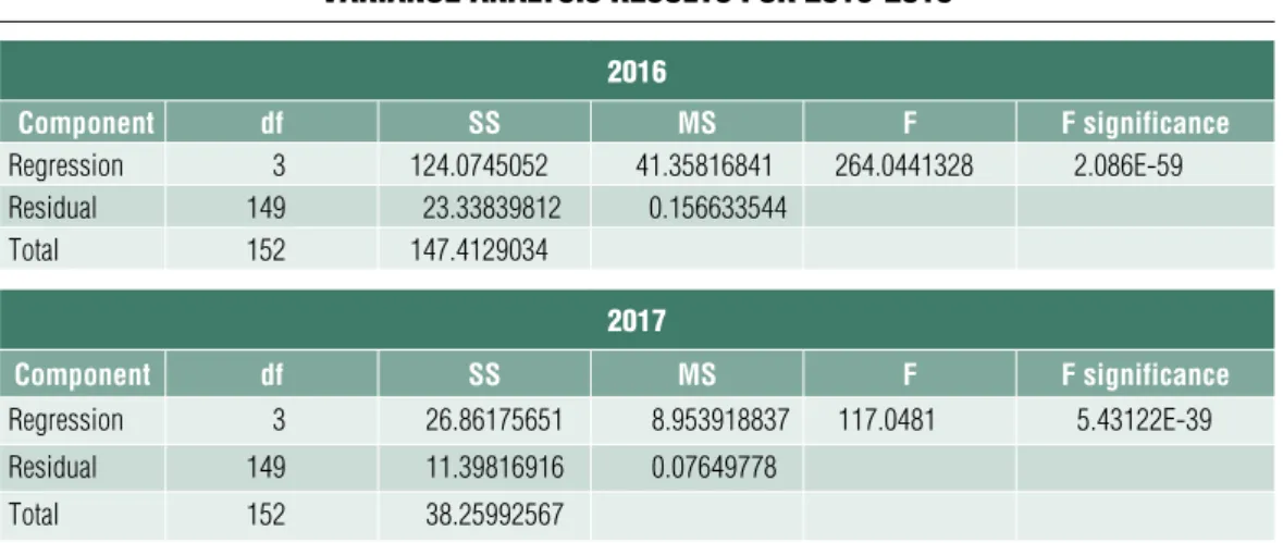
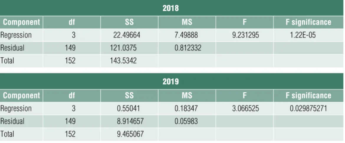
The variance analysis results for 2016-2019 are shown in Table 2.

Based on the variance analysis tables the null hypothesis is rejected; therefore, there is at least one explanatory variable with significant effect, and at least one regression parameter whose value is other than zero.

The results for regression coefficients between 2016-2019 are shown in Table 3.

Table 2 varianCe analysis results for 2016-2019

2016

Component df SS MS F F significance

regression 3 124.0745052 41.35816841 264.0441328 2.086E-59

residual 149 23.33839812 0.156633544

total 152 147.4129034

2017

regression 3 26.86175651 8.953918837 117.0481 5.43122E-39

residual 149 11.39816916 0.07649778

total 152 38.25992567

(12)

Table 3 results for regression CoeffiCients between 2016-2019

2016 Coefficients standard error t-value p-value lower 95% upper 95%

intercept 0.008 0.035 0.234 0.815 -0.060 0.077

1/A_it –1 746.389 90.993 8.203 0.000 566.586 926.193

(ΔREV_it – ΔREC_it)/A_it –1 0.022 0.026 0.842 0.401 -0.029 0.073

PPE_it/A_it –1 -0.329 0.012 -27.012 0.000 -0.353 -0.305

intercept 0.179 0.027 6.554 0.000 0.125 0.233

1/A_it –1 -120.455 121.416 -0.992 0.323 -360.374 119.464

(ΔREV_it – ΔREC_it)/A_it –1 -0.088 0.008 -11.531 0.000 -0.103 -0.073

PPE_it/A_it –1 -0.454 0.025 -18.295 0.000 -0.503 -0.405

intercept -0.005 0.078 -0.058 0.954 -0.159 0.150

1/A_it –1 -112.443 159.107 -0.707 0.481 -426,841 201.955

(ΔREV_it – ΔREC_it)/A_it –1 -0.054 0.096 -0.562 0.575 -0.244 0.136

PPE_it/A_it –1 -0.052 0.010 -5.149 0.000 -0.072 -0.032

intercept 0.027 0.032 0.828 0.409 -0.037 0.090

1/A_it –1 -87.937 35.950 -2.446 0.016 -158.975 -16.900

(ΔREV_it – ΔREC_it)/A_it –1 0.045 0.042 1.061 0.290 -0.039 0.128

PPE_it/A_it –1 -0.074 0.054 -1.381 0.169 -0.180 0.032

2018

regression 3 22.49664 7.49888 9.231295 1.22E-05

residual 149 121.0375 0.812332

total 152 143.5342

2019

regression 3 0.55041 0.18347 3.066525 0.029875271

residual 149 8.914657 0.05983

total 152 9.465067

(13)

The regression analysis shows that the estimated coefficients of property, plant and equipment (PPE_it/A_it-1) assumed negative values in all four examined periods, as expected, because property, plant and equipment are linked to an income-decreasing accrual-based approach (i.e. amortisation cost). As for the expected value of change in revenues minus change in receivables it can be seen that in 2017 and 2018 the company managers made income-decreasing accrual-based decisions, while in 2016 and 2019 the results suggest income-increasing accrual based-decisions.

Analysing the coefficients of determination, the relationship between variables appears to be strong in 2016 and 2017, and weak in 2018 and 2019, as demonstrated in Table 4.

Based on the figures of the table the regression function appears not to fit well in years 2018 and 2019.

conclusions

The hypothesis tests of earnings management are based on the firm-specific expectation

models used for estimating ‘normal’ total accruals. These models facilitate changes in nondiscretionary accruals that are caused by shifting economic circumstances. In the empirical study of manufacturing companies active in Baranya county the assumption that neither income-decreasing nor income- increasing accrual-based decisions are made should be rejected. This can be supported by the results obtained through the DeAngelo model. Most of the examined entities are considered to be micro and small companies with less chance of accounting manipulation. The results show that the managers exercise discretion over accruals driven by their own ideas. The income- decreasing effects of discretionary accruals are greater than the income-increasing effects. The obtained results are indicative.

However, further examinations are needed to ensure reliability. As a possible direction of research, additional quality measurement models should be involved, with the conduct of a nationwide empirical study applying clear delimitation in order to substantiate the current conclusions. ■

Table 4 CoeffiCients of determination between 2016-2019

2016 2017 2018 2019

r² 0.841680 0.702086 0.156734 0.058152

Note

1 In the original research data was collected for 237 companies. Of these 23 companies were deleted due to incomplete data, 15 companies pursued non-manufacturing activity based on NACE classification, 10 companies had no closing data for fiscal year 2019, and 36 companies had no closing data for fiscal year 2015 and/or 2016.

(14)

References Aren, s. (2003). Yöneticilerin Kar Yönetimi İle İlgili Tutumlarɪ ve IMKB’de Bir uygulama [Managers’ Attitudes Regarding Profit Management and an Application in IMKB]. Doctoral Thesis, Gebze Yüksek Teknoloji Enstitüsü Yayɪnlangmamiş

Ball, R., shivakmar, L. (2008). Earnings Quality at Initial Public offerings. Journal of Accounting and Economics, Volume, 45, Issues 2-3, pp. 324–349, https://doi.org/10.1016/j.jacceco.2007.12.001

Bedőházi Z.-R. (2009). A Nemzetközi Pénzügyi Beszámolási standarok alkalmazásának hatása a Magyar Tőzsdén jegyzett vállalatok számiviteli minőségére [The impact of using IFRS on the accounting quality of firms listed on the Hungarian Stock Exchange]. PhD dissertation, Pécs

Beest, f., Braam, G., Boelens, s. (2009).

Quality of financial Reporting: Measuring Qualitative characteristics. NiCE Working Paper pp. 09–108, https://www.researchgate.net/

publication/254877109_Quality_of_financial_

reporting_measuring_qualitative_characteristics cheung, E., Evans, E., Wright, s. (2010). A Historical Review of Quality in financial Reporting in Australia. Pacific Accounting Review, Volume 22, Issue 2,

https://doi.org/10.1108/01140581011074520 crosby, f. B. (1995). Quality without Tears. New York, McGraw Hill

Davidson, s., stickney, c., Weil, R. (1985).

Intermediate Accounting: concepts, Methods and use (fourth Ed.) Forthworth: Dryden Press

DeAngelo, L. E. (1986). Accounting Numbers as Market Valuation substitutes:

A study of Management Buyouts of Public

stockholders. Accounting Review, Volume 61, Issue 3, pp. 400–420, https://shibbolethsp.jstor.

org/start?entityID=https%3A%2f%2fidp.

pte.hu%2fsaml2%2fidp%2fmetadata.php&

dest=https://www.jstor.org/stable/247149&site=

jstor

Dechow, P. M., sloan, R. G. (1991). Executive Incentives and the Horizon Problem: An Empirical Investigation. Journal of Accounting and Economics, Volume 14, Issue 1, pp. 51–89,

https://doi.org/10.1016/0167-7187(91)90058-s Dechow, P. M., sloan, R. G., sweeney, A. P.

(1995). Detecting Earnings Management. Accounting Review, Volume 70, Issue 2, pp. 193–225, https://

shibbolethsp.jstor.org/start?entityID=https%3A%2 f%2fidp.pte.hu%2fsaml2%2fidp%2fmetadata.

php&dest=https://www.jstor.org/stable/248303&

site=jstor

Dechow, P., Weili, G., schrand, c. (2010).

understanding Earnings Quality: A Review of the Proxies, their Determinants and their consequences, Journal of Accounting and Economics, Volume 50, Issues 2–3, pp. 344–401,

https://doi.org/10.1016/j.jacceco.2010.09.001 Defond, M. L., Jiambalvo, J. (1994). Debt covenant Violation and Manipulation of Accruals.

Journal of Accounting and Economics, Volume 17, Issue 1–2, pp. 145–176,

https://doi.org/10.1016/0165-4101(94)90008-6 Downen, T. (2014). Defining and Measuring financial Reporting Precision. Journal of Theo- retical Accounting Research, Volume 9, Issue 2, pp.

21–57,

https://doi.org/10.2139/ssrn.2129263

Duman, H. (2010). The Practices of Earnings Management Effect over the Quality of financial

(15)

Reporting and company’s Performance in the Principle of Disclosure: An Application In IMKB. Doctoral Thesis, Selçuk Üniversitesi, Yayɪnlangmamiş

Ervin, L., Keith, f., Tracy, s. (1998). Earnings Management using Asset sales: An International study of countries Allowing Noncurrent Asset Revaluation. Journal of Business Finance and Accounting, Volume 25, Issue 9–10, pp. 1287–

1317,

https://doi.org/10.1111/1468-5957.00239

Gajevszky, A. (2015). Assessing financial Reporting Quality: Evidence from Romania. Audit finaciar, Volume 13, Issue 121, pp. 69–80

Gill-De-Albornoz, B., Illueca, M. (2005).

Earnings Management under Price Regulation:

Empirical Evidence from the spanish Electricity Industry. Energy Economics, Volume 27, Issue 2, pp.

279–304,

https://doi.org/10.1016/j.eneco.2004.12.005 Healy, M., Wahlen, M. (1999). A Review of the Earnings Management Literature and its Implications for standard setting. Accounting Horizons, Volume 13, Issue 4, pp. 365–383, https://doi.org/10.2308/acch.1999.13.4.365

Healy, P. M. (1985). The Effect of Bonus schemes on Accounting Decisions. Journal of Accounting and Economics, Volume 7, Issue 1–3, pp. 85–

107,

https://doi.org/10.1016/0165-4101(85)90029-1 Holthausen, R. W., Larcker, D. f., sloan, R. G. (1995). Annual Bonus schemes and the Manipulation of Earnings. Journal of Accounting and Economics, Volume 19, Issue 1, pp. 29–74, https://doi.org/10.1016/0165-4101(94)00376-G

Jaggi, B., Lee, P. (2002). Earnings Management Response to Debt covenant Violations and Debt

Restructuring. Journal of Accounting, Auditing and Finance, Volume 17, Issue 1, pp. 295–

324,

https://doi.org/10.1177/0148558X0201700402 Jones, J. (1991). Earnings Management During Import Relief Investigations. Journal of Accounting Research, Volume 29, Issue 2, pp. 193–228, https://doi.org/10.2307/2491047

Keating, A., Zimmerman, J. (2000).

Depreciation-policy changes: Tax, Earnings Management, and Investment opportunity Incentives. Journal of Accounting and Economics, Volume 28, Issue 3, pp. 359–389,

https://doi.org/10.1016/s0165-4101(00)00004-5 Noriaki K., seraku N., Takahashi f. (1984).

Attractive Quality and Must-be Quality. Journal of the Japanese Society for Quality Control. Volume 14, Issue 2, pp. 39–48

Robb, W. (2014). The Effect of Analysts’

forecasts on Earnings Management in financial Institutions. The Journal of Financial Research, Volume 21, Issue 3, pp. 315–331,

https://doi.org/10.1111/j.1475-6803.1998.tb00688.x Taguchi, G. (1992). Taguchi on Robust Technology Development: Bringing Quality Engineering upstream. ASME Press,

https://doi.org/10.1115/1.800288

Teshima, N., shuto, A. (2008). Managerial ownership and Earnings Management. Theory and Empirical Evidence from Japan. Journal of International Financial Management and Accounting, Volume 19, Issue 1, pp. 107–132,

https://doi.org/10.1111/j.1467-646X.2008.01018.x Tóth, G., széles, Zs. (2020). A Big4 könyv- vizsgáló cégek számviteli minőségre gyakorolt hatásának összehasonlító elemzése [A Comparative Analysis of the Impact of Big4 Audit Firms on

(16)

Accounting Quality]. Válság & kilábalás: Innovatív megoldások. Konferenciakötet

Vörös, J. (2010). Termelés- és szolgáltatás- menedzsment [Production and Service Management], Akadémiai Kiadó, Budapest

Willekens, M. (2008). Effects of External Auditing in Privately Held companies: Empirical Evidence from Belgium. Working Paper Series, https://

www.coursehero.com/file/247084/Willekens- 2008/