Polynomial approximation in several variables ∗
Vilmos Totik
†Dedicated to Zeev Ditzian
Abstract
This paper is about the characterization of the rate of best polynomial approximation on a domain inRdby multivariate polynomials of degreen via a suitable modulus of continuity or smoothness. We shall be concerned with the situations: approximation on convex polytopes and approxima- tion on (not necessarily convex) smooth algebraic domains. We shall introduce appropriate moduli of smoothness and prove the corresponding Jackson theorem. The usual weak converses are also true.
Contents
I Approximation on polytopes 2
1 The main result 2
2 Outline of the proof of Theorem 1.1 5
3 Pyramidal covering and approximation on general polytopes 6 3.1 Lemmas on geometry and polynomial partitions . . . 7 3.2 Pyramidal coverings . . . 12 List of notations used in the pyramidal covering construction . . 15 3.3 Patching approximants on a pyramidal covering together to a
global approximant . . . 16 4 Approximation on pyramids and the proof of Theorem 1.1 for
large degrees 17
5 Small degrees 26
II Approximation on algebraic domains 27
∗AMS Classification: 41A10, 41A17 Keywords: polynomials, several variables, approxima- tion, moduli of smoothness, polytopes, algebraic domains
†Supported by ERC Advanced Grant No. 267055 and by NSF DMS 1564541
6 Domains and moduli of smoothness 28 6.1 Domains inR2 . . . 28 6.2 Domains inRd . . . 30 6.3 The Jackson theorem and its converse . . . 30 7 Reduction to approximation close to the boundary 32
8 Ther= 1 case 38
9 Approximation on disks 41
10 A detour on the derivative of composite functions 45
11 Proof of Theorem 6.5 48
One of the primary questions of approximation theory is to characterize the rate of approximation by a given system in terms of some (computable) modulus of continuity or smoothness. In this spirit we set out the task to characterize the rate of best polynomial approximation on a domain inRd by multivariate polynomials of degreenvia a suitable modulus of continuity or smoothness.
We shall be concerned with the situations: approximation on convex poly- topes and approximation on (not necessarily convex) smooth algebraic domains.
We shall introduce appropriate moduli of smoothness and prove the correspond- ing Jackson theorem. The usual weak converses are also true, they actually au- tomatically follow from classical converse results and from the way the moduli of smoothness are defined.
Part I
Approximation on polytopes
In this first part we shall be concerned with convex polytopes in any dimension.
1 The main result
Letf be a continuous function on [−1,1]. Withϕ(x) =√
1−x2andr= 1,2, . . . let
ωϕr(f, δ) = sup
0<h≤δ, x∈[−1,1]|∆rhϕ(x)f(x)| (1.1) be its so calledϕ-modulus of smoothness of orderr, where
∆rhf(x) =
r
X
k=0
(−1)k r
k
f x+ (r
2−k)h
(1.2)
is the r-th symmetric difference. In (1.1) it is agreed that ∆rhf(x) = 0 if [x−
r
2h, x+r2h] 6⊆[−1,1]. See the book [6] for this kind of moduli of smoothness, for their properties and for their applications.
With this modulus of smoothness one can characterize the rate of best poly- nomial approximation on [−1,1]. Indeed, if
En(f) = inf
Pnkf−Pnk[−1,1]
is the error (in the supremum norm) of the best polynomial approximation by polynomials of degree at mostn, then the Jackson-type estimate
En(f)≤Crωϕr(f,1/n), as well as its weak converse
ωϕr(f,1/n)≤Cr
1 nr
n
X
k=0
(k+ 1)r−1Ek(f) (1.3) are true (see [6, Theorem 7.2.1] and [6, Theorem 7.2.4]). Our aim in this paper is to find the analogues of these in several variables.
In Rd we call a closed set K ⊂ Rd a convex polytope if it is the convex hull of finitely many points. K isd-dimensional if it has an inner point, which we shall always assume. The analogue of the ϕ-modulus of smoothness onK was defined in [6, Chapter 12], and to recall its definition we need to consider the given function along lines in different directions. A direction e in Rd is just a unit vectore∈Rd. Clearly, e can be identified with an element of the unit sphereSd−1, so Sd−1 is the set of all directions inRd. LetKbe a convex polytope, x ∈ K and e ∈ Sd−1 a direction. The line le,x through x which is parallel with e intersects K in a segment Ae,xBe,x. The role of ϕ on that segment is taken over by
d˜K(e, x) =q
dist(x, Ae,x)·dist(x, Be,x). (1.4) Iff is a continuous function onK, then we define itsr-th symmetric differ- ences in the direction ofeas
∆rhef(x) =
r
X
k=0
(−1)k r
k
f x+ (r
2−k)he
(1.5) with the agreement that this is 0 ifx+r2heorx−r2hedoes not belong toK.
If E is a set of directions, then the r-th modulus of smoothness with these directions is defined as (see [6, Section 12.2])
ωrK(f, δ)E = sup
e∈E, h≤δ, x∈K |∆rhd˜
K(e,x)ef(x)|. (1.6) If E is the direction of the edges of K, then we shall simply write ωKr(f, δ) forωrK(f, δ)E. These moduli of smoothness share many properties of classical moduli, in particular
ωrK(f, λδ)E ≤CrλrωKr(f, δ)E
for anyλ≥1. We shall also frequently use monotonicity inK: ifK1⊂K2then ωrK1(f, δ)E ≤ωKr2(f, δ)E, which is immediate from the definitions.
Note that whenK= [−1,1], then there is only one direction (and its nega- tive) and this modulus of smoothness takes the form (1.1), i.e.
ωϕr(f, δ) =ωr[−1,1](f, δ). (1.7) Let Πdn be the set of polynomials in d-variables of total degree at most n, and let the supremum norm on a setK be denoted byk · kK. For a continuous functionf ∈C(K) we are interested in
En(f)K = inf
Pn∈Πdnkf−PnkK, (1.8) which is the error of best approximation off by polynomials of total degree at mostn.
In the first part of this paper we prove
Theorem 1.1 If K is a convex polytope in Rd, then forr= 1,2, . . .
En(f)K≤CωKr(f,1/n), n≥rd. (1.9) Here the constantC depends only onK andr.
Call a polytopeK inRd a simple polytope if at every vertex there are pre- ciselydedges. Theorem 1.1 was verified in [6, Theorem 12.1.1] for cubes/paral- lelepipeds in all dimensions, and in [6, Theorem 12.2.3] (with an additional term) for all simple polytopes. The somewhat weaker result
En(f)K ≤CωrK(f,1/n)Sd−1, (1.10) i.e. when all directions are used in the modulus of smoothness, was proven in [14, Chapters 1-10] for all polytopes in R3. In [14, Chapter 11, Theorem 1.1], it was also stated that (1.10) holds also in Rd, d > 3, but Andriy Prymak noticed that the proof (that reduced the problem to approximation on simple polytopes) does not give that, so the claim was wrong in the sense that the proof in [14, Chapter 11] yields (1.10) only for special polytopesK (which satisfy the property that the intersection ofK with any hyperplane that cuts off a vertex is a simple (d−1)-dimensional polytope). Thus, in its generality, (1.9) (which also covers (1.10)) is new (and actually sharper than what has been previously proven in the special cases known in the literature).
The weak converse
ωrK(f,1/n)≤Cr
1 nr
n
X
k=0
(k+ 1)r−1Ek(f)K,
is an immediate consequence of (1.3) if we take into account how the modulus of smoothness on the left has been defined.
The Jackson-type estimate Theorem 1.1 and the weak converse (1.3) easily imply the following. IfK1⊂Kis a segment and we considerf only onK1, then
we obtain a continuous function on a segment/interval, and we can consider the approximation of this one-variable function by polynomials of the same (single) variable. Now it follows that ifα > 0 and the error of best approximation of f on any segment of K by (one variable) polynomials of degree at most n is
≤n−α, then on the whole K the function f can be approximated with error
≤ Cn−α by polynomials (of several variables) of degree at most n (where C depends only onK).
Remark 1.2 We need to say a few words on the degree of polynomials. In this work we use total degree (i.e. the degree ofxα11· · ·xαdd is α1+· · ·+αd), while the works [6] and [14] used maximal degree in the separate variables (in which case the degree ofxα11· · ·xαddis maxαj). This has not much effect on the corresponding Jackson theorem, only on the range ofnfor which the theorem holds. Indeed, let En(f) be as in (1.8) where the infimum is taken for all polynomials of total degree at mostn, and let
En∗(f)K = inf
Qnkf−QnkK,
where now the infimum is taken for all polynomials Qn that are of degree at mostn in each variable. It is clear thatEnd(f)K ≤En∗(f)K ≤En(f)K, so a Jackson-type estimate for either ofEn orEn∗ yields a Jackson-type estimate for the other. Note however, that if f0 is the polynomial xr1−1· · ·xrd−1 and K is the unit cube in Rd, then En∗(f0) = 0 for n ≥ r−1 while En(f0) = 0 only forn≥d(r−1). In a similar manner, if we use edge directions in forming the modulus of smoothness, thenωr(f0, δ)K ≡0, so when usingEn(f) the Jackson- type estimate (1.9) cannot hold forn < d(r−1). That is why we claimed (1.9) only forn≥rd.
2 Outline of the proof of Theorem 1.1
In the proof of Theorem 1.1 a special role is played by pyramids. Let S0 be a convex (d−1)-dimensional polytope in Rd, and P ∈ Rd a point outside the hyperplane of S0. The convex hull of S0 and P determines a d-dimensional pyramidS with apex atP. We callS0 the base ofS, and the edges emanating fromP the apex edges ofS.
LetK ⊂Rd be a convexd-dimensional polytope with vertices {Qj}mj=1. If Qj is a vertex ofKandLis a hyperplane that intersects all the edges emanating fromQj, thenLcuts off a pyramidSj from Kwith apex atQj (and with base K∩L).
As has been mentioned, (1.10) was proven in [14] inR3. That proof works in any dimension for a polytope K which has the property that if we cut off a small pyramidSj around every vertexQj, then what remains (say K0) is a simple polytope (note that inR2 any polytope is simple, so the just mentioned property is true for any 3-dimensional polytopes). In that approach simple polytopes are used in two essential ways.
• 1)K0is simple, so for it the claim (say (1.10)) on the rate of approximation is true by [6, Theorem 12.2.3] (with the additional term in that theorem separately removed).
• 2) IfSλj is theλ-shrunk copy ofSj from Qj, then the truncated pyramid Sj\Sjλ is simple, so for it the claim on the rate of approximation is true again by [6, Theorem 12.2.3].
Note that if we are working in R3, then no assumption is needed, K0 is always simple, so the just outlined approach yields the theorem. This is no longer true inRd,d >3 (an observation by A. Prymak1), so the use of simple polytopes in 1)–2) must be avoided. The proof we give is by induction on the dimension, but for the induction we need the approximants to be given by linear operators, and the modulus of smoothness should involve only edge-directions.
A) In 2) the truncated pyramid is (for λ <1 close to 1) the union of well- overlapped product sets (with the smaller base of the truncated pyramid × the edges), so induction and simple patching gives the result for the truncated pyramid. From there the proof in [14] gives the result for each of the pyramids Sj.
B) The problem in 1) is avoided by not looking at all on the remaining poly- topeK0, but rather appropriately covering the original polytope by translated copies of the pyramidsSj and patching the approximants on them (which were established in A) together.
We start with the last tusk, i.e. by constructing an appropriate pyramidal covering.
3 Pyramidal covering and approximation on gen- eral polytopes
We shall writean ≺bn if there is a C >0 such that for sufficiently large nwe have|an| ≤Cbn. If we also specify a rangen≥n0forn, then an≺bn,n≥n0
means that there is aC >0 for which|an| ≤Cbn for alln≥n0.
We shall prove Theorem 1.1 using bounded linear operators mappingC(K) into Πdn (since Πdn is finite dimensional, it does not matter what norm is used on Πdn). Therefore, we introduce the notation
EnL(f)K≺ω(1/n) (3.1)
to denote the fact that for all sufficiently largen (independent off) there are bounded linear operatorsLn:C(K)→Πdn such that
kf−LnfkK≤Cω(1/n). (3.2)
1Indeed, ifV is a non-simple polytope inRd−1,d >3, andKis the convex hull inRdof V and the point (0, . . . ,0,1)∈Rd, then for any hyperplaneLinRdthat is parallel with the xd= 0 hyperplane that intersectsKin at least two points the intersectionK∩Lis similar toV, henceLcuts off a non-simple pyramid fromK.
with some constantC independent off andn. Sometimes we need to specify a subclassCofC(K) for which (3.2) is required, in which case we write
EnL(f)K ≺ω(1/n), f ∈ C. (3.3) (3.1) proves Theorem 1.1 for sufficiently largen. Smalln’s will be separately handled in Theorem 5.1 in Section 5.
In this section we show that if one can approximate in the correct order on pyramids, then the approximation on any polytope follows by a pyramidal covering of the polytope. Then, in the next section, we show how to handle pyramids.
We shall need some simple geometric facts.
3.1 Lemmas on geometry and polynomial partitions
Lemma 3.1 For every convex bodyS⊂Rd there is a constantα >0 with the following property: if we representS as the intersection of half spaces, then for any pointP in Rd the distance fromP to one of these half spaces is at least α times the distance fromP toS.
Proof. Let us write a ballBr of some radiusr inside S about a point O of S, and letR be such that the ball BR about O of radius R contains S in its interior. We show that for anyβ <1 the numberα=βr/Ris suitable.
Indeed, letP be any point outsideS. TheOP segment intersects the bound- ary ofS at a pointQ(see Figure 1). Then P Q≥dist(P, S), so if we select the pointqon the segment P Qclose toQ, then P q≥βdist(P, S) and at the same time Oq < Rare satisfied (note that Q lies inside BR, so we may select q so that it also lies inside that ball). There is a half spaceK among the given half spaces that containsS but does not contain the pointq. LetH be the bound- ary of that half space. ThenH intersects theOP segment in a pointA (that lies necessarily on the segmentQq), and consider the normal line to H at the point A. This normal line and the line passing through O and P determines a planeL that intersectsH in a line ℓ (see below for the case when these two lines coincide). Let B be the closest point of ℓ to O and C the closest point of ℓ to P. Since L is perpendicular toH and P ∈L, the distance from P to C is precisely the distance fromP to the half spaceK. Furthermore,OB ≥r (K contains the ballBr),OA < R (A lies on the segmentQq which lies inside BR), and from the similarity of the triangles ACP and ABO we obtain that P C/P A = OB/OA > r/R. Since P A ≥ P q ≥ β dist(P, S) is also true, we finally obtain
dist(P, K) =P C >(r/R)P A≥(r/R)βdist(P, S).
The just given proof used that the normal line toH atAand the line passing through O and P are different (so they form a plane). If they are the same, then dist(P, K) =P A≥P q≥βdist(P, S).
S
O Br
Q q P
A B l
C
Figure 1:
Lemma 3.2 LetS be a convex polytope lying in the unit ballB1(0)ofRd, and letε >0. There is a constantk =k(S, ε) such that for every n≥1 there are polynomialsRkn of degree at most knfor which
a) 0≤Rkn(x)≤1 forx∈B1(0), b) 1−Rkn(x)≤2−n forx∈S,
c) Rkn(x)≤2−n forx∈B1(0),dist(x, S)≥ε.
Remark 3.3 1. The lemma is closely related to well localized polynomial par- titions of unity. Indeed, ifS1, . . . , Sm are finitely many closed convex bodies in B1(0) andU1, . . . , Umare neighborhoods of them, then there is a constantθ >0 and for each largenthere are polynomials P1,n, . . . , Pm,n, Pm+1,n of degree at mostnsuch that
• 0≤Pj,n≤1 onB1(0) for allj,
• Pm+1
j=1 Pj,n≡1,
• Pj,n≤θn onB1(0)\Uj for all 1≤j≤mand
• Pm+1,n≤θn on∪mj=1Sj.
In particular, if theSj are pairwise disjoint, then (by choosingUj to lie outside
∪s6=jSs) we can also have (with a possibly largeθ)
• 1−θn≤Pj≤1 onSj for all 1≤j≤m.
Indeed, to see that, we may assume that each Sj is a convex polytope (just place such a polytope in between Sj andUj). Then we can apply Lemma 3.2 to eachSj (with anε for which theε-neighborhood of Sj is part of Uj) to get polynomials Rj,n/m of degree at most n/m as in Lemma 3.2 (just apply the lemma withnreplaced byn/km). Now it is easy to see that
Pj,n=Rj,n/m(1−R1,n/m)· · ·(1−Rj−1,n/m), j = 1, . . . , m and
Pm+1,n= (1−R1,n/m)· · ·(1−Rm,n/m)
satisfy the requirements. The θ depends onm, εand on the numbers k(Sj, ε) in Lemma 3.2.
2. To our knowledge in more than one variables polynomial partitions of unity were created for the fist time in [7] (that paper dealt with dimension 2).
There the decrease was of power type away from the sets, and that decrease started right at the boundary of the setsSj. In the just given constructionPj,n
tends to 0 geometrically fast outsideUj, though there is no information on its behavior in Uj\Sj. In patching local polynomial approximants together to a global approximant one needs, in general, a geometric rate of convergence to 0 as just has been explained.
Proof of of Lemma 3.2. Letα >0 be the constant from Lemma 3.1 for the polytopeS.
It is well known (see e.g. [12, Corollary VI.3.6]) that for every ε >0 there are ansand for everynpolynomials ˜Rsn(x1) of a single variablex1of degreesn such that 0≤R˜sn≤1 on [−3,3], 1−R˜sn≤3−n on [−3,0] and ˜Rsn≤3−n on [αε,3]. We regard ˜Rsnas a polynomial of degreesnof the variables (x1, . . . , xd).
S is the intersection of some half-spacesK1, . . . , Km. We may assume that the boundary of eachKj contains a point ofS. If Φj is an isometry ofRd that mapsKj into the half-spacex1≤0, then ˜Rsn(Φj(x)) is a polynomial of degree at mostsn, it is in between 0 and 1 on the unit ball (note that the unit ball is mapped into the strip−3≤x1 ≤3 by Φj), it is closer to 1 than 3−n onS (S is mapped into −3 ≤ x1 ≤0) and it is closer to 0 than 3−n at any point of B1(0)\Kj which lies of distance ≥ αε from Kj. However, by the choice ofα, any point in the unit ball that is of distance ≥εfrom S lies of distance
≥αεfrom one of theseKj, hence, the product of the polynomials ˜Rsn(Φj(x)), j= 1, . . . , m, is appropriate in the lemma for sufficiently large n.
Lemma 3.4 Let S ⊂ K be convex polytopes in Rd, and let Sε be the closed ε-neighborhood ofS. Let furthermoreH ⊂K be a closed set such that for some δ >0 the intersectionS∩H contains a (d-dimensional) ball of radius δ. Then for everyl0 there is anl such that
ElL0n(f)Sε∩K ≺ω(1/n), ElL0n(f)H ≺ω(1/n), f ∈C(K) (3.4)
imply
ELln(f)S∪H ≺ω(1/n), f ∈C(K). (3.5) Here the constant in the last≺does not depend onf, it depends only on the diameter ofK, onδand on the constants in the preceding two≺. The quantity ω(1/n) is a generic term that tends to 0 asn→ ∞— we shall use the lemma with ω(1/n) replaced by the 1/n-value of a certain modulus of smoothness. Recall also our convention that the implication (3.4) ⇒ (3.5) is not for individual functions, but should be read that if (3.4), i.e.
ElL0n(f)Sε∩K ≤C0ω(1/n), ELl0n(f)H≤C0ω(1/n), n≥n0
holds for all functionsf ∈C(K) with some constants C0, n0, then (3.5), i.e.
ELln(f)S∪H ≤C1ω(1/n), n≥n1
is also true with someC1, n1for all such f.
Proof. We may assumeK⊂B1(0), i.e. thatK lies in the unit ball ofRd. First we recall
Lemma 3.5 [14, Lemma 4.1] If B is a ball of radius δ lying in the unit ball B1(0), then for any polynomialQn of degree at mostn
kQnkB1(0)≤ kQnkB(4/δ)n. (3.6) LetP1,n andP2,nbe bounded linear operators onC(K) mapping into Πdl0n such that
kf−P1,nfkSε∩K≤Cω(1/n), kf−P2,nfkH≤Cω(1/n)
forf ∈C(K). By assumption there is a ballB ⊆H∩S of some radiusδ >0, and on that ball we have
kP1,nf−P2,nfkB≤ kf−P2,nfkH+kf−P1,nfkSε∩K ≤2Cω(1/n), hence, by Lemma 3.5
kP1,nf−P2,nfkB1(0)≤2C(4/δ)l0nω(1/n). (3.7) Choose an integer b such that (1/2)b < (δ/4)l0 and with the polynomials Rkn from Lemma 3.2 forS and withl= (l0+kb) set
Llnf =RkbnP1,nf+ (1−Rkbn)P2,nf.
This is a bounded linear operator fromC(K) to Πdln, and for it we have
• onH∩Sε
|f −Llnf| ≤Rkbn|f−P1,nf|+ (1−Rkbn)|f−P2,nf| ≤Cω(1/n), (3.8)
• onS (see (3.7))
|f−Llnf| = |f−P1,nf+ (1−Rkbn)(P1,nf−P2,nf)| ≤ |f−P1,nf|+ + (1−Rkbn)|P1,nf−P2,nf| ≤Cω(1/n) + 2−bn2C(4/δ)l0nω(1/n)
≤ 3Cω(1/n), (3.9)
• and onH\Sε
|f−Llnf| = |(f−P2,nf −Rkbn(P1,nf−P2,nf)| ≤ |f −P2,nf|
+ Rkbn|P1,nf−P2,nf| ≤Cω(1/n) + 2−bn2C(4/δ)l0nω(1/n)
≤ 3Cω(1/n). (3.10)
The inequalities (3.8)–(3.10) verify the lemma.
As usual, we identify a pointQ∈Rd with its position vector−−→OQ, whereO is the origin.
Let ΦQ,η be the homothetic transformation of Rd with center at Q and with dilation factor η, i.e. ΦQ,η is the linear transformation of Rd for which ΦQ,η(P) =Q+η(P−Q) for anyP ∈Rd.
LetK be a convex polytope inRdwith vertices Q1, . . . , Qm. Lemma 3.6 K is covered by the setsΦQj,d/(d+1)K,j= 1, . . . , m.
Proof. By taking a simplicial decomposition2 of K into d-dimensional sim- plices with vertices from the set {Q1, . . . , Qm}, we may assume that K is a simplex (so m = d+ 1). Then any point X in K is of the form X = α1Q1+· · ·αd+1Qd+1 with αj ≥ 0, P
αj = 1. Here one of the αj’s, say α1, is at least 1/(d+ 1), hence from the representation
X = (1−α1) α2
1−α1Q2+· · ·+ λd+1
1−α1Qd+1
+α1Q1=: (1−α1)Y +α1Q1
we can see that X divides the segment Y Q1 into segments with length-ratio α1/(1−α1) ≥ 1/d, which implies that X belongs to ΦQ1,d/(d+1)K because Y ∈K.
2Actually, all we need is Caratheodory’s theorem that any point of the convex hull of a setH inRdlies in the convex hull of some of its (d+ 1) points, so ifKis a polytope inRd, then it is the union of the simplices spanned by (d+ 1) vertices ofK.
Lemma 3.7 Let K be as in the preceding lemma and let 0 < θ < 1/(d+ 1) be fixed. IfP is any point of ΦQj,1−θK and we translateΦQj,θK by the vector
−−→QjP, then the translated polytope is part of K.
Proof. Indeed, if R is any point of ΦQj,θK and we denote the vectors−−→QjP and−−→QjR byv andu, respectively, then Qj+ (1−θ)−1v, Qj+θ−1ubelong to K, hence so does the point (1−θ)(Qj+ (1−θ)−1v) +θ(Qj+θ−1u) on their connecting segment. But this point isQj+u+v =R+u=R+−−→QjP, which means that ΦQj,θK+−−→QjP ⊂K. This proof also gives that if P lies in thed- dimensional interior of ΦQj,1−θK, then the translated polytope ΦQj,θK+−−→QjP also lies in the interior ofK.
What we have just proven can be applied on every lower dimensional face of K. Indeed, let Fk be a k-dimensional face of K that contains Qj. Since Fk∩ΦQj,θK = ΦQj,θFk, what we have just established can be applied to the face Fk and to ΦQj,θFk. Thus, if P ∈ ΦQj,1−θK is on the face Fk, then the face ΦQj,θFk+−−→QjP of the translated polytope ΦQj,θK+−−→QjP lies inFk, and ifP lies in thek-dimensional interior of ΦQj,1−θFk, thenFk∩(ΦQj,θK+−−→QjP) lies in the k-dimensional interior of Fk. In the latter case if P′ lies in the k dimensional interior ofFk∩(ΦQj,θK+−−→QjP), then we can enlarge ΦQj,θK+−−→QjP from P′ by a factor 1 +τ > 1 with some small τ > 0 so that the enlarged polytope is still part ofK. Furthermore, this enlarged polytope then contains the intersection of a neighborhood of ΦQj,θK+−−→QjP with Fk (note however, that it does not contain ad-dimensional neighborhood of ΦQj,θK+−−→QjP since all points of Fk ∩(ΦQj,θK +−−→QjP) lie on the boundary — actually on the correspondingk-dimensional face — of the enlarged polytope).
3.2 Pyramidal coverings
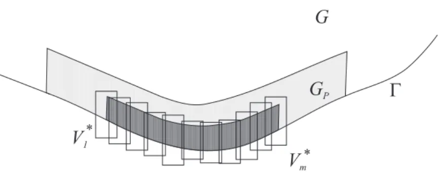
In this section we describe a covering of a polytope K by pyramids Ks with the property that there is a listing of the elementsKsin the covering in which consecutive elements have relatively large intersections (the intersection of their interiors is non-empty). This covering will then allow us in the next subsection, by repeatedly applying the results from the preceding subsection, to obtain a global polynomial approximant onK(to a given functionf) from approximants on theKs. In this way we reduce the problem of polynomial approximation on Kto approximation on (the) pyramids (Ks).
Since the construction is rather involved with many notations, for the sake of the reader we shall list the notations in a separate subsection at the end of this section.
Let K and Qj as before, and fix 0 < θ <1/(d+ 1). Around each Qj we cut off fromK a small pyramidSj with vertex atQj by a (d−1)-dimensional
Ks
Sj Sj,h
Sj, /2h
ws vs
Figure 2: A schematic figure of the setsSj,Sj,η,Sj,η/2,Ks,Kη,s(lightly shaded figure) andKη/2,s (dark shaded figure), as well as the vectorsvs, ws.
hyperplane. We assume that for eachj we haveSj⊂ΦQj,θK, and we fix these Sj in the following discussion.
For simplicity let us also writeSj,η for the homothetic copy ΦQj,ηSj. Letη <1/2 be given. We shall deal with the following type of setsKs,Kη,s
andKη/2,s, 1≤s≤T, whereT will be given during the construction below.
• EachKs=Sj+vsis a translated copy of someSj by a translation vector vs,
• Kη,s⊂Sj,1/2+vs is the translation of theη-size copy Sj,η of Sj by the same vectorvs, and
• Kη/2,s⊆Kη,sis a translation of the smallerSj,η/2 by a possibly different vectorws.
See Figure 2. For emphasis we use calligraphic letter inKη/2,s to indicate that the vertex ofKη/2,smay be at a different point than the common vertices ofKs
andKη,s.
By an η-pyramid covering of K we mean a covering K = ∪Ts=1Ks, where each Ks is a translated copy of one of the Sj’s, and which has the following properties: there are anε > 0 and related subpyramidsKη,s, Kη/2,s of Ks as just described such that
(i) eachKsis contained inK and eachKη/2,s is contained in Kη,s, (ii) K=∪Ts=1Kη/2,s,
(iii) the intersection of the interiors ofKη/2,sandKη/2,s+1is non-empty for all s= 1, . . . , T −1,
(iv) Kεη/2,s∩K⊂Kη,s, whereKη/2,sε is the closedε-neighborhood ofKη/2,s. Proposition 3.8 For everyη <1/2 there is an η-pyramid covering ofK.
Proof. We say that a finite setX ⊂K is τ-dense in K if every point ofK lies closer to some point ofX thanτ.
We define for some small 0< τ aτ-dense setX onKas follows. First of all, letX1 be the set of all vertices Qj of K. Then for every edgeF1 ofK extend F1∩X1 to aτ-dense set ofF1. X1 and the added points for all edges formX2. Then for every 2 dimensional faceF2 of K extendF2∩X2 to aτ-dense set of F2, etc. keep extending the point setsXk using higher and higher dimensional faces. This way we get aτ-dense setXd−1 on the boundary ofK, and finally extend that to aτ-dense set onK.
First we define the setsKη/2,s. IfP ∈X andP belongs to ΦQj,1−θK(there must be such a j in view of Lemma 3.6) then let KP be the translation of Sj,η/2 = ΦQj,η/2Sj by the vector −−→QjP. If for a P there are more than one j withP ∈ΦQj,1−θK, then get aKP for all such j. We show that the collection of all theseKP generate a suitableη-pyramid covering by repeating eachKP a few times (to meet the requirement in (iii)). According to Lemma 3.7 we have Sj+−−→QjP ⊂K (recall thatSj ⊂ΦQj,θK), and sinceη <1/2 we also have
KP ⊂Sj,1/2+−−→QjP ⊂Sj+−−→QjP ⊂K. (3.11) If τ is sufficiently small, then these KP cover K. Indeed, from how X was constructed it is clear that the vertices, and hence small neighborhoods (relative to K) of them are covered (note that each Qj belongs to X, so Sj,η/2 is one of theKP’s). Then each edge F1, and hence a small neighborhood (relative to K) of F1 is covered (this neighborhood depends only onη and not onτ), and so on, we continue with higher and higher dimensional faces and their small neighborhoods, and finally with all ofK. This proves (ii).
We also get that for small τ >0 the interiors Int(KP) of the pyramids KP
cover the interior Int(K) of K. At this point we need the following simple lemma.
Lemma 3.9 Let G be a connected set and suppose thatG=∪iGi, whereGi are finitely many open sets. Let{Gi}i be the vertices of a graph, and connect in that graph the verticesGiandGj if for the setsGi,Gj we haveGi∩ Gj6=∅. Then this graph is connected.
This lemma says that in any coveringG =∪iGi of a connected open setG by open setsGi, for any index pairsk6=l there are indicesi0, ij, . . . , imwith some msuch thati0=k,im=l, and for any 0≤j < mwe haveGij ∩ Gij+1 6=∅. Proof. For clearer notation let us write GVj if we talk aboutGj as a vertex of the graph. LetV1, . . . , Vrbe the vertex sets of the connected components of the graph (i.e. eachVs is a non-empty set of certainGjV, Vs1∩Vs2=∅ fors16=s2,
and eachGVj belongs to one of theVs). Each∪GVj∈ViGjis open, and for different componentsVi these sets are disjoint. Now the conclusion follows from the fact that a connected set cannot be the disjoint union of non-empty open sets.
Since the just constructed graph for Int(K) and{Int(KP)}P∈Xis connected, there is a path in it which goes through every vertex. In other words, there is a listingKη/2,s, s= 1, . . . , T, of all theKP’s (maybe with repetition) in which Kη/2,s∩ Kη/2,s+1 contains a ball for alls < T. This proves (iii).
We still need to define the sets Kη,s and Ks, see Figure 2. Consider a Kη/2,s = KP, say it is Sj,η/2+−−→QjP (i.e. the vector ws in the definition of pyramidal covering is−−→QjP in this case). IfP is the vertexQj, then enlargeKP
fromP by a factor 2 to getKη,s. However, ifP is not a vertex ofK, then there is a smallest dimensional faceFk ofK such thatP lies in the interior Intk(Fk) ofFk (ifFk isk-dimensional, then Intk(Fk) denotes itsk-dimensional interior), where we considerK itself as the d-dimensional face of K. Hence, according to what was said after Lemma 3.7,Fk∩(Sj,η+−−→QjP) also lies in Intk(Fk). Let Q∈Intk(Fk∩Sj,η) be a point lying in thek-dimensional interior ofFk∩Sj,η. ThenQ+−−→QjP lies in thek-dimensional interior Intk(Fk∩(Sj,η+−−→QjP)) of the faceFk∩(Sj,η+−−→QjP) ofSj,η+−−→QjP, and the translation of Intk(Fk∩(Sj,η+−−→QjP)) by the vector−−→QQj will containFk∩KP ifQ lies sufficiently close to Qj (and at the same time this translation is contained inFk). Thus, if we set
Kη,s=Sj,η+−−→QP
(i.e. the vectorvsin the pyramidal covering is−−→QP), then thisKη,sis such that it contains the intersection of a neighborhood ofKη/2,s=KP withK, proving (iv).
Finally, with the previous notations we setKs=Sj+−−→QP, which is part of K(see Lemma 3.7), so (i) holds.
List of notations used in the pyramidal covering construction
For the sake of the reader we repeat here in a concised form the notations used in the pyramidal covering.
ΦQ,η – homothetic transformation with center atQand dilation factorη Qj – vertices ofK
Sj (⊂K) – small pyramids cut off fromK with vertex atSj
Sj,η – the homothetic copy ΦQj,ηSj ofSj
Ks– anSj+vswith a translation vectorvs Kη,s– Sj,η+vswith the same translation vectorvs
Kη/2,s (⊂Kη,s) –Sj,η/2+ws with another translation vectorws
3.3 Patching approximants on a pyramidal covering to- gether to a global approximant
Let ˜ωrSj(f,1/n) be the modulus of smoothness onSj when only the directions in the apex edges ofSjare used. We shall use again the notationSj,ηfor ΦQj,ηSj. Proposition 3.10 If for eachj= 1, . . . , m we have
EnL(f)Sj,2η ≺ω˜rSj(f,1/n), f ∈C(Sj), (3.12) then there is anl such that
ELln(f)K ≺ωrK(f,1/n), f ∈C(K).
Recall that here, on the right hand side, the modulus of smoothness uses the edge directions ofK.
Proof. LetK=∪Ts=1Ksbe anη-pyramid covering ofKas in Proposition 3.8, and setHt=∪ts=1Kη/2,s. With induction we are going to prove that for every 1≤t≤T there is anl for which
ElnL(f)Ht ≺ωrK(f,1/n). (3.13) The claim then follows by settingt=T.
For t = 1 the set H1 = Kη/2,1 is an Sj,η/2+w1 for some j and some vectorw1,K1=Sj+v1 with the same j and with another vectorv1, and the correspondingKη,1 isSj,η+v1. Note thatKη,1 is contained inSj,1/2+v1. By the assumption (make a homothecy with factor 2 and a translation byv1) there are linear operatorsLn :C(Sj,1/2+v1)→Πdn such that
kf−LnfkSj,η+v1 ≺ω˜rSj,1/2+v
1(f,1/n). (3.14)
SinceKη/2,1=Sj,η/2+w1 is part ofSj,η+v1(see property (i) of theη-pyramid covering), and the right-hand side in (3.14) is at mostωKr(f,1/n) (note that all apex-edge directions ofSj+v1 are also edge directions ofK), we obtain
kf−LnfkKη/2,1=kf−LnfkSj,η/2+w1 ≺ωrK(f,1/n), (3.15) and hence the claim follows in this case.
The induction step is a consequence of Lemma 3.4. Indeed, if (3.13) is known fort−1 (t >1), say
ElL0n(f)Ht−1 ≺ωKr(f,1/n), (3.16) then letH =Ht−1,S =Kη/2,tin Lemma 3.4, and setω(1/n) =ωrK(f,1/n) there (note that by property (iii) of theη-pyramidal coveringH∩S=Ht−1∩Kη/2,t⊇ Kη/2,t−1∩Kη/2,tcontains a ball). As we have just seen (see the argument leading to (3.14)–(3.15)), (3.12) implies
EnL(f)Kη,t ≺ωKr(f,1/n).
Furthermore, by property (iv) of an η-pyramid covering, for some ε > 0 the relative (with respect toK) neighborhoodKη/2,tε ∩K ofKη/2,t is part ofKη,t, hence we obtain
EnL(f)Kεη/2,t∩K≺ωrK(f,1/n), and together with this also
ElL0n(f)Kεη/2,t∩K≺ωKr(f,1/n).
Now the claim follows fort(i.e. forHt=Ht−1∪Kη/2,t) in view of this estimate, (3.16) and Lemma 3.4.
4 Approximation on pyramids and the proof of Theorem 1.1 for large degrees
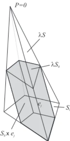
LetS0 be a (d−1)-dimensional convex polytope lying in the hyperplaneH of RdandS the convex hull ofS0∪ {P}, where P is a point outsideH (soS is a ddimensional pyramid with apex atP). Recall that the edges ofS emanating fromP are called apex edges.
Assume that P = 0. Let λH be the hyperplane that we obtain from H by a dilation with factor 0 < λ <1 and center P = 0. ThenλH cutsS into two parts, the pyramid λS and the polytope Uλ :=S \λS such that S0 and λS0are (d−1)-dimensional similar faces ofUλ. Lete1, . . . , embe the segments connecting the corresponding points ofS0and λS0. These segments lie on the apex edges ofS, on each apex edge lying one of them. IfEis the endpoint ofej
lying inλS0, then the product set (λS0)×ej is defined as the union of all the translationsej+−−→EM, whereM runs through the points ofλS0 (see Figure 3).
Proposition 4.1 Ifλ >(d−1)/d, then the product sets(λS0)×ej,1≤j≤m have a common interior and their union isUλ.
Proof. Let the vertices of S0 be Q1, . . . , Qm. Then the vertices of λS are λQ1, . . . , λQm, and we may assume thatej=Qj(λQj). As before, let ΦQj,µS0
be the homothetic image ofS0 with factorµand dilation center atQj.
LetZ be any point in Uλ, andℓZ be the half-line from the origin through Z. ThisℓZ intersects S0 in a point X, and by Lemma 3.6 X ∈ΦQj,(d−1)/dS0
for some 1≤j ≤m. IfZ =σX, thenλ≤σ≤1, andZ ∈ΦσQj,(d−1)/d(σS0).
However, this latter set is aσ(d−1)/dsize copy (ΦQj,σ(d−1)/d(Sj)) ofS0trans- lated by the vector−−−−−−→Qj(σQj), so it is contained in theλ > σ(d−1)/dsize copy ΦQj,λS0 ofS0 translated by the same vector−−−−−−→Qj(σQj).
The translation of λS0 by the vector −−−−−−→(λQj)Qj is ΦQj,λS0, and the product set (λS0)×ej is precisely the set of points that lie in one of the translations of λS0 by a vector −−−−−−−−→(λQj)(τ Qj), λ≤τ ≤1. But then, in view of −−−−−−→Qj(σQj) =
P=0
S0
lS0
lS0xej
ej
lS
Figure 3: The pyramidS, its baseS0and theirλ-dilations from the apexP = 0.
The shaded slab is the product setλS0×ej.
−−−−−−→
Qj(λQj)+−−−−−−−−→(λQj)(σQj), what we have just proven means thatZis in this product set (λS0)×ej.
The claim that the product sets (λS0)×ej have a common interior point is trivial, since ifY lies in the (d−1)-dimensional interior ofλS0, then all points of Uλ=S\λSthat lie sufficiently close toY lie in all the product sets (λS0)×ej.
Remark 4.2 Easy modification of the proof gives that if 1> λ >(d−1)/d and µ <1,µλ > (d−1)/d, then for µ sufficiently close to 1 even the product sets ΦλQj,µ(λS0)×ej, 1≤j ≤m have a common interior and their union is Uλ.3 For these sets it is clearly true that for smallε >0
ΦλQj,µ(λS0)×ej
ε
∩Uλ⊂(λS0)×ej, (4.1) where·ε denotes ε-neighborhood.
Proposition 4.3 Suppose that S0 is a polytope in Rd−1 for which there are bounded linear operatorsVn :C(S0)→Πdn−1 such that
kf−VnfkS0 ≺ωrS0(f,1/n)E,
3Actually, the claim is true for allµ <1 withµλ >(d−1)/d. Indeed, in view of Proposition 4.1 we need to prove only that the convex sets ΦλQj,(d−1)/dλS0have non-empty intersection.
For this the following simple argument was communicated to the author by J´anos Kincses. In view of Helly’s theorem all these sets have non-empty intersection if anydof them have non- empty intersection (note that we are working now in ad−1 dimensional hyperplane ofRd).
However, ifj1, . . . , jdare different indices, then the center of mass of the ((d−1)-dimensional) simplex ∆ determined byλQj1, . . . , λQjd lies in all ΦλQjs,(d−1)/dλS0,s= 1, . . . , d, because the center of mass divides the segment from any vertexQjsthrough the center of mass to the opposite face of ∆ in the ration 1 : (d−1).
where ωrS0(f, δ)E is a modulus of smoothness on S0 using some directions E. Then there is a sequence of bounded linear operators Ln :C(S0×[0,1])→Πdn such that
kf−LnfkS0×[0,1]≺ωSr0×[0,1](f,1/n)E∪{ed}, whereed is thed-th unit vector inRd (perpendicular toRd−1).
Proof. In view of Remark 1.2 it is sufficient to construct the linear operators Ln with the required properties except thatLnf can be a polynomial of degree at mostnin each variable (as opposed to the claim whereLnf has total degree at mostn).
This is basically [6, Section 12.1]. Indeed, it was proven there that for everyr there areUn :C[0,1]→Π1nsuch thatUnare uniformly bounded linear operators fromC[0,1] toC[0,1] with the property that
kf −Unfk[0,1] ≺ωr[0,1](f,1/n) (recall also (1.7)).
Let y = (y1, . . . , yd−1). For a function f(y, x) define fx(y) = f(y, x) and fy(x) =f(y, x). Then
ωS0×[0,1](f, δ)E∪{ed}= max sup
x∈[0,1]
ωS0(fx, δ)E,sup
y∈S0
ω[0,1](fy, δ)
! .
When we applyVnin the variabley∈S0, then we denote it byVny. Let now Lnf =Unx◦Vnyfx. The functionVnyfxis of the formP
ki≤nak,n(x)yk11· · ·ydk−d−11 where k = (k1, . . . , kd−1), and here eachak,n(x) is continuous because Vn are bounded linear operators. Hence, the linearity ofUn yields that Lnf is of the formP
ki≤nUnx(ak,n(x))yk11· · ·ydd−d−11, which is a polynomial of degree at mostn in each of the variablesy1, . . . , yd−1, x. Now
|Lnf(y, x)−f(y, x)| ≤ |Unx◦Vnyfx(y)−Unxfx(y)|+|Unxfx(y)−fx(y)|. With some fixedC, C1, C2 for all largenthe first term on the right is
|Unx◦Vnyfx(y)−Unxfx(y)| = |Unx(Vnyfx(y)−fx(y))|
≤ Csup
x |Vnyfx(y)−fx(y))|
≤ C1sup
x ωS0(fx,1/n)E ≤C1ωS0×[0,1](f,1/n)E∪{ed}, while for each fixedy∈S0the second term is
|Unxfy(x)−fy(x)| ≤C2ω[0,1](fy,1/n)≤CωS0×[0,1](f,1/n)E∪{ed}.
The preceding proposition says that if we can prove a Jackson-type inequality on a setK0via bounded linear operators, then a similar Jackson-type theorem holds on the product spaceK0×[0,1]. By applying an affine transformation we obtain that the same is true for product sets of the formK0×e, whereeis not necessarily perpendicular to the hyperspace ofK0 (but lies outside it). In particular, we can apply this to all the product sets (λS0)×ej from Proposition 4.1 above, and we obtain that if
EnL(f)S0≺ωrS0(f,1/n), (4.2) (which implies the same for the setλS0 replacingS0sinceλS0 is a homothetic image ofS0) whereωSr0(f, δ) is the modulus of smoothness onS0using the edge directionsS0, then for eachj = 1, . . . , mwe have
EnL(f)(λS0)×ej ≺ωr(λS0)×ej(f,1/n).
Let us return now to the pyramidS and to its decompositionS =λS∪Uλ
from the beginning of this section. If we combine the just discussed relation with the fact (4.1) and apply Lemma 3.4 repeatedly withω(1/n) =ωrUλ(f,1/n), H =∪tj=1−1ΦλQj,µ(λS0)×ej, S= ΦλQt,µ(λS0)×et,t= 1, . . . , m, andK =Uλ, then we can conclude that (4.2) implies that there is anlsuch that
ElnL(f)Uλ ≺ωrUλ(f,1/n).
If this is true for all n with ln≥ nr (where nr is some number), then we have proved
Proposition 4.4 Under the assumption (4.2) there is annr such that EnL(F)Uλ ≺ωUrλ(F,1/n), n≥nr.
Recall our convention that this means that for all functionsF continuous onUλ
we have
ELn(F)Uλ ≤C0ωUrλ(F,1/n), n≥nr
with some constantC0 independent ofF.
Since both sides are homothetic invariant, we also have EbnL(F)qUλ ≺ωrqUλ(F,1/bn), bn≥nr. for anyq >0 andb >0.
In particular, if E is the set of the apex edge directions of S and for some functionF and numbersq, b >0
ωrqUλ(F,1/bn)≺ωSr(f,1/n)E (4.3) also holds, then we can conclude
EbnL(F)qUλ ≺ωSr(f,1/n)E, bn≥nr. (4.4) Now we are ready to prove Theorem 1.1 for large degreesn.
We shall prove it in the form