MTA DOKTORI ÉRTEKEZÉS Szabó Endre 2013

(1)

MTA DOKTORI ´ ERTEKEZ´ ES

Szab´ o Endre

2013

(2)

(3)

DISSERTATION

Application of Algebraic Geometry in Combinatorics and in Group Theory

Szab´ o Endre

R´ enyi Alfr´ ed Matematikai Institute of Mathematics

2013

(4)

(5)

Overview

In this Dissertation we discuss the following three important, inter- twined themes, and their applications. Here we list the three themes together with the most important results we prove about them.

1. Bounding the number of incidences.

The basic problem is to find upper bound on the number of incidences among p points and q geometric figures. The main result of the Dissertation on this theme is Theorem 6, which generalises (among other things) the famous Szemer´edi–Trotter theorem.

2. How to find groups?

We study when does it happen that among three timesngeometric figures we can find Cn² occurrences of certain three-figure configurations. We find that typically there is a large symmetry-group responsible for the too-many coincidences. The main results of the Dissertation on this theme are Theorems 14 and 15. They are related (among other things) to Hrushovski’s Group Configuration Theorem [75] and the recent paper of Tao [156].

3. Growth in groups.

For finite subsets α of a group we study how the size of its powers αⁿvary in terms ofn. We are especially interested in the structure of subsets with slowly growingαⁿ. The main results of the Disser- tation on this theme are Theorems 16, 17 and 18. They are closely related (among many other things) to the Freiman–Ruzsa theorem, and the results of Helfgott [72], Breuillard–Green–Tao [27], Bourgain- Gamburd [12].

The first two of the themes are of combinatorial flavor, the last one belongs to group theory. Although it does not appear as a separate chapter, algebraic geometry has a crucial role in all three themes.

In the Dissertation there are several interesting applications of the above results.

4. Applications in combinatorics.

• Corollary 19 improves significantly the best known exponent in a problem of Hirzebruch [74].

• Theorem 20 answers a question of Erd˝os, Lov´asz and Veszter- gombi [51].

• Corollary 24 solves a conjecture of Sz´ekely (see [42, Conjecture 3.41]). Moreover, Theorem 23 is a vast generalisation of this conjecture.

• Theorem 26 partially solves a variation of the so called Orchard problem (see [83, 152]).

3

(8)

4 OVERVIEW

5. Applications in group theory.

• Corollary 27 solves the conjecture of Babai [7] for simple groups of bounded rank.

• Theorem 29 solves the conjecture of Liebeck, Nikolov and Shalev [99]

for simple groups of bounded rank. Theorem 30 is a variation on the same theme.

• Theorem 33 solves the conjecture of Weiss [170] in the class of BCP(r) groups.

The Dissertation’s place among related areas of mathematics In this section I will try to position the main results of this Dissertation in their mathematical vicinity.

The first theme is bounding various incidence numbers. Our starting point is the following famous theorem of Szemer´edi–Trotter [154]. Among p points andq lines in the plane there are at mostO

p^2/3q^2/3+p+q incidences. Several generalisations of this result emerged since then, bounding the number of incidences amongppoints andqgeometric figures (instead of lines). Let me list a few just to get a feeling for it. Pach–Sharir [120]

(see Theorem 1) bounds incidence numbers for plane curves; Chazelle–

Edelsbrunner–Guibas–Sharir [31] and Solymosi–Tao [145] studies hyperplanes in the euclidean space Rⁿ; T´oth Csaba [162] deals with complex lines inC²; Bourgain–Katz–Tao [15], and Bourgain [10] estimates incidence numbers concerning lines, and certain hyperbolas in the projective plane over the finite field F_p for any prime p. Theorem 6 in this Dissertation is a higher dimensional generalisation. It bounds the number of incidences among ppoints and q subvarieties of bounded degree inRⁿorCⁿ. It would be interesting to extend this result to finite fields as well, but this direction is still wide open. Theorem 6 is the most important link between our first and second theme, we use it to exclude certain kind of degeneracies during the construction of groups.

Our second theme is a very general phenomenon in mathematics. If in a geometric situation there are many unexpected coincidences then we may expect a large symmetry-group lurking in the background. There is a vast number of variations on this theme, here we mention only two results. In his Group Configuration Theorem [75](see also [122]) Hrushovski consid- ers a model-theoretic scenario. He constructs symmetry-groups in extreme generality. Roughly it goes like this. Let us consider astable¹mathematical theory T, and two d-dimensional² families³ of “function-like” two-variable

1Stability of a mathematical theory T essentially means, that in the models of T there aren’t too many “types” of elements.

2In model-theory, under appropriate conditions, one can define an extremely general notion of dimension similar to the Krull-dimension used in algebra.

3Members of afamilyare parametrised by an index set. The dimension of the family is the dimension of this index set.

(9)

THE DISSERTATION’S PLACE AMONG RELATED AREAS OF MATHEMATICS 5

relations⁴ in a model ofT. The direct product of the two index sets is 2d- dimensional, so we expect to get a 2d-dimensional family of pairwise compositions.⁵ If the compositions form instead a d-dimensional family,⁶ then both families can be induced from a group in the following manner. In the theoryT one can define a setXequipped with the action of ad-dimensional group Gof symmetries, and both families “essentially look like” the family R_g of relations onXdefined by the formulaR_g=

(x, y)∈X×X

y=gx} (where g runs through the elements of G). The special case of the Group Configuration theorem where T is the theory of algebraically closed fields, which is reproduced in the Dissertation as Lemma 1.3.6, plays an important role in the proof of Theorem 14 and Theorem 15.

While the result of Hrushovski has a rather “continuous nature”, in Theorem 14 and Theorem 15 we face a combinatorial situation, and find similar consequences. The precursor of this two theorems is a paper of Elekes–R´onyai [45] (where the group of symmetries does not yet appear explicitly). An interesting new development is the work of Tao [156], where he studies the phenomenon that, ifA, B are “very large” subsets of a finite field, andP is a two-variate polynomial, then the setP(A, B) is “typically”

fills up almost the whole field. The exceptional polynomials, analogously to our Theorem 14 and Theorem 15, are just the reparametrisations of either the addition, or the multiplication, so they originate from the additive or the multiplicative group of the field. Tao even mentions in his blog [157]

that the “Elekes–Szab´o theory”, as he puts it, may have an important role in the further investigation of his problem.

It is worth noting here that the finite point-configurations appearing in Theorem 14 and Theorem 15 show up also in the group obtained there, and one can see easily that they form a non-growing subset of that group. A finite subsetα of a group is called non-growing if its third power,⁷ denoted by α³, has size at mostK|α|.

With this last comment we have arrived at our third theme, the study of non-growing subsets of groups. The theme is interesting for commutative as well as non-commutative groups, and both versions have plenty of applications within and outside of group-theory (see later). It is quite remarkable how the commutative and non-commutative worlds intertwine, and inter- act with each other in these investigations. Even though they study rather different-looking phenomena, they borrow a large number of ideas and methods from each other.

We begin with the commutative groups. The Freiman–Ruzsa theorem [55] (see also [138] for the proof given by Ruzsa) is a fundamental result in additive combinatorics. It is the following. If α ⊆ Z is a finite

4It means that almost allxare related to a bounded number ofyonly.

5Thecomposition of two relationsRandS is the relation defined by the formula (x, z)

∃y: (x, y)∈Rand (y, z)∈S

6Typically all compositions are different, they form a 2d-dimensional family. Some- times there are coincidences, and we may get a smaller dimension. Our case is the “max- imal degeneration”.

7 αⁿdenotes the set of alln-term products formed from the elements ofα.

(10)

6 OVERVIEW

subset such that α+α

≤K|α| holds,⁸ thenα can be covered by a d(K)- dimensional generalised arithmetic progression of sizef(K)|α|. Later Green and Ruzsa [65] generalised the theorem for arbitrary abelian group. In this generality a non-growing subsetαcan be covered by the sum of a generalised arithmetic progression and a finite subgroup. (This kind of sums are called coset progressions.) The most important open question in this direction is, whether one can find a description of non-growing sets such that the parameters (like the f(K) above) depend on K polynomially. For example, is it true that all non-growing setsα⊆Zⁿ₂ can be covered by at mostCK^mcosets of a subgroup of size at most|α|(whereC andmare constants independent of everything)?

After this detour on commutative structures let us return to the world of not necessarily commutative groups. Letα be a non-growing set in a group.

What can we say about the structure of α? The first, and at the same time the most well-known result in this direction is the theorem of Gromov [67].

The size ofαⁿcan be bounded from above⁹by a polynomial ofnif and only if the subgroup generated byαisvirtually nilpotent.¹⁰ (Here the polynomial may depend on the group.)

The next breakthrough in the study of non-growing sets was the theorem of Helfgott [72]. Letαbe a generating system in thegroupSL(2, p),¹¹(where p is an arbitrary prime). Then either α grows exponentially, i.e

α³ ≥

|α|^1+ε for some constant εindependent of everything, or α³ =G (so there is no room for further expansion).¹² A strong motivation for Helfgott was that his theorem implies immediately the Babai conjecture for the groups SL(2, p) (see Corollary 27). Later it turned out that Helfgott’s theorem can be significantly extended. According to the Product theorem, the same statement is valid in the groupsSL(n, q) for arbitrary prime-powerq.¹³ The importance of the Product theorem is indicated by the fact that it was proved independently at the same time by two different groups: Breuillard–

Green–Tao [25] and Pyber–Szab´o [133].

In the last few years there were a lot of advances in understanding the structure of non-growing sets. Here we mention two of them only.

Breuillard–Green–Tao [27] studied non-growing subsets of arbitrary groups.

8It follows from the Pl¨unecke–Ruzsa estimates that in this case|α+α+α| ≤K²|α|, i.e. αis non-growing. In non-commutative groups this reasoning fails, this is why we insisted on bounding the size of α³. Interestingly, in arbitrary groups, the size of the higher powers ofαcan be bounded in terms of

α³ .

9In Gromov’s theorem we bound all powers ofα, not justα³ as above.

10A group isvirtually nilpotent if it has a nilpotent subgroup of finite index.

11for a prime p,SL(n, p) denotes the group of thosen×n matrices of determinant 1, whose entries are taken from thep-element fieldFp(i.e. the ring of remainder-classes modulop); the group operation is the multiplication of matrices. More generally, ifqis a power of a prime, andFis an arbitrary field, thenSL(n, q) andSL(n,F) denote the groups of thosen×nmatrices of determinant 1, whose entries are taken from theq-element field Fqand the fieldFrespectively.)

12Instead ofα³=G, Helfgott proved only thatα^k=Gwith an appropriate valuek.

13In fact the Product theorem deals with all simple subgroups ofSL(n, q), hence all finite simple groups but the alternating groups. The constant ε depends only onn(i.e.

the rank of the group).

(11)

THE DISSERTATION’S PLACE AMONG RELATED AREAS OF MATHEMATICS 7

Their result is a common generalisation of Gromov’s theorem and the Freiman–

Ruzsa theorem. If α is a non-growing subset of a group (i.e.

α³

≤K|α|), then the subsetα^d(K)contains a subgroupHfor which, in the corresponding factor group¹⁴ the image ofα can be covered by f(K) translates of an ap- propriatenil-progression.¹⁵ Perhaps the only downside of their description is that their method does not give us bounds on the size ofd(K) andf(K). For future applications in combinatorics and number theory however it would be important to know thatd(K) andf(K) are polynomial functions ofK at least for a certain classes of groups.¹⁶ This was precisely the goal (to obtain polynomial bounds) we aimed at with L´aszl´o Pyber in our paper [131]. We proved (see Theorem 18) that if α is a symmetric¹⁷ non-growing subset in the groupSL(n,F) (over an arbitrary field F), thenα⁶ contains a subgroup H for which, in the corresponding factor group¹⁴ the image of α can be covered by f(K) translates of an appropriate soluble subgroup, wheref(K) is a polynomial function of K whose degree and coefficients depend on n.

So far the most impressive application of the Product theorem is the so-called “Bourgain–Gamburd expansion machine”. The method was devel- oped by Bourgain and Gamburd for the construction of expander graphs.¹⁸ (The expander graphs have important applications, e.g., in computer sci- ence.) Bourgain and Gamburd proved in [12] that, for every girthgthere is an ε >0 for which, all those Cayley-graphs¹⁹of the groups SL(2, p) having girth larger thatgareε-expander. When the paper [12] was born, Helfgott’s theorem was the state of art. This is why they had to limit themselves to the groups SL(2, p). Later with the same method, using the Product theorem, a large number of new expander families were constructed (see for example Breuillard–Green–Tao [26] and [22], Varjú [165], Bourgain–Varjú [17]), and also Golsefidy–Varjú [62]). Expander graphs are used in number theory in the so-called “affine sieve methods” (see, e.g., Bourgain–Gamburd–

Sarnak [14]). In fact, the original motivation for [12] came from this kind of sieve methods.

The Sum-product theorem²⁰ (Erd˝os–Szemer´edi [53]) and its numerous variations (see, e.g., Tao [159] and the references given there) form an important chapter in additive combinatorics. Even though the Sum-product type theorems do not appear in this Dissertation, still they are strongly related to some of our themes. Elekes [40] has shown that the Sum-product theorem follows from the Szemer´edi–Trotter theorem (see also Solymosi [144]). The

14More precisely, in the quotient group of the normaliser ofH byH.

15 The nil-progressions are the counterparts of generalised arithmetic progressions living in nilpotent groups. Often it is enough to know that the image ofαin that quotient group can be covered by at mostf(K) translates of a nilpotent subgroup.

16The Product theorem can also be rewritten in a similar form (valid for the class of finite simple groups of bounded rank), and indeed, in that version the constants depend on Kpolynomially . A number of existing applications depend crucially on this polynomiality.

17A subsetαof a group issymmetric, if for each elementa∈αwe havea⁻¹ ∈α.

18A graph onnvertices is calledε-expander, if any setX of vertices of size|X| ≤ ⁿ₂ is adjacent to at leastε|X|further vertices outsideX.

19TheCayley-graphof a groupGcorresponding to a generating setαhas vertex-set G, and two verticesx, y∈Gare connected with an edge if and only ifxy⁻¹ ∈α.

20IfAis a finite set of real numbers then max |A+A|,|A·A|

≥c|A|^1+ε.

(12)

8 OVERVIEW

other way around, Bourgain–Katz–Tao [16] started with a Sum-product type theorem, and proved a Szemer´edi–Trotter type theorem. Helfgott’s theorem (on the group SL(2, p) was originally proved in [72] using a Sum- product type theorem, and even today many researchers think of the Prod- uct theorem as a kind of “non-commutative Sum-product-like theorem”.

Actually, the proof of the Product theorem follows a different path, but the Sum-product type theorems still have an important role in the study of non- growing subsets (see, e.g., Gill–Helfgott [59]). This connection works in the other direction as well. (Commutative) Sum-product type theorems can be proved using the (non-commutative) Product theorem (see, e.g., Breuillard–

Green–Tao [25, Chapter 8]).

It is worth mentioning a recent result of Bourgain [10], which is in close relation with our themes. He used the above mentioned “expansion- machine” methods to prove a Szemer´edi–Trotter type bound for certain hyperbolas in a finite geometry.

The structure of the Dissertation

The Dissertation is based on seven articles, and each of these articles corresponds to one chapter of the Dissertation. At the moment when I’m writing, three of the articles ( [48], [46], [125] ) have already appeared in print, one of them ( [133] ) is submitted and another one ( [61] ) is already accepted for publication, and two of them ( [47], [131] ) are still in preprint form.

• [48] and [47] are joint papers with Gy¨orgy Elekes, they correspond to Chapter 1 and Chapter 5 of the Dissertation.

• [46] is a joint paper with Gy¨orgy Elekes an Mikl´os Simonovits, it corresponds to Chapter 4 of the Dissertation.

• [133] and [131] are joint works with L´aszl´o Pyber, they correspond to Chapter 2 and Chapter 3 of the Dissertation.

• [125] is a joint work with Cheryl Praeger, L´aszl´o Pyber and Pablo Spiga, it corresponds to Chapter 6 of the Dissertation.

• [61] is a joint work with Nick Gill, L´aszl´o Pyber, and Ian Short, it corresponds to Chapter 7 of the Dissertation.

The chapters of the Dissertation are essentially equivalent to the original papers, but I unified references, and tried to eliminate inconsistent notations.

In those cases when one chapter uses a theorem proved in another chapter, instead of just giving a reference, I preferred to fully restate the theorem in the form most appropriate for the application. Therefore the chapters are self-contained, one can read them separately. Each chapter has its own introductory section where the history and the context is explained in detail.

In addition, the rest of this Overview serves as a (somewhat informal) guide to the main results of the Dissertation. It is organised along our main themes, as follows.

1. Bounding the number of incidences.

Section 1.2 belongs here, which is part of the paper [48].

Our main result in this area is Theorem 6.

(13)

1. BOUNDING THE NUMBER OF INCIDENCES 9

Section 1.1 and Section 1.4 belong here.

Our main results in this area are Theorem 14, and Theorem 15.

3. Growth in groups.

Chapter 2 and Chapter 3 belong here.

Our main results in this area are Theorem 16, and Theorem 18.

4. Applications in combinatorics.

Chapter 5, Chapter 4, and Section 1.5 belong here.

Our most important results in this area are Theorem 20, Theo- rem 23, Theorem 26, and Corollary 24.

5. Applications in group theory.

Chapter 7 and Chapter 6 belong here.

Our most important results in this area are Theorem 29, Theo- rem 30, and Theorem 33.

1. Bounding the number of incidences

Good upper bounds on the number of incidences play a central role in combinatorial geometry, and in the theory of geometric algorithms. (Re- cently they have shown up is additive combinatorics as well, see [40, 44, 42].) The first result of this type is the Szemer´edi–Trotter theorem [154], which was later extended by Pach and Sharir for continuous plane curves.

Theorem 1 (Pach–Sharir [120]). Let Γ be a family of simple²¹continuous plane curves such that any two have at mostM points in common, and there are at most scurves of Γpassing through any point in the plane (i.e. Γ has s degrees of freedom). Then the number of incidences amongppoints and q curves of Γ is at most

(1.1) C

p^s/(2s⁻¹⁾q^(2s⁻^2)/(2s⁻¹⁾+p+q ,

where the constant factor C depends only on s and M. In the special case when Γ is the family of lines in the plane, we have s= 2,M = 1, hence we obtain the original Szemer´edi–Trotter theorem.

We need the following notation.

Definition 2. Let X be an arbitrary set (it could be say R^N, the N- dimensional space), P ⊆X be a subset, and Qbe a collection of subsets of X. (We think of the elements of Q as if they were “geometric shapes” in X.)

• I(P, Q) denotes the number of incidences in the (P, Q) system, i.e. the number of pairs (p, q)∈P×Qwhere the point pbelongs to the subsetq.

• For an arbitrary pointt∈P we denote byQ_t⊆Qthe collection of those members of Qthat contain t.

Let us consider now the configuration in R³ that consists ofp collinear points, andqplanes containing all of theppoints. The number of incidences in this configuration is pq. If we are looking for a bound similar to (1.1) that is valid for configurations in Rⁿ, then we will need some kind of non- degeneracy assumption to avoid this type of configurations. The following

21A curve issimple if it has no self-intersection.

(14)

10 OVERVIEW

definition refines this idea. It allows a few sub-configurations of this type, provided that they are small enough. The parameterband the combinatorial dimension kregulates how many and how large “bad parts” do we allow in our configuration. Later in all of our upper bounds the constant factors will depend on both band k, but the exponents may depend on konly. (It was an interesting problem on its own right to find a non-degeneracy condition that is sufficiently “generous” to be satisfied in a large number of interesting geometric situations.)

Definition 3(Combinatorial dimension, recursive definition). We fix a constant b >0. LetX be an arbitrary set, P ⊆X a subset, andQ a collection of subsets of X. We say that cdim_b(P, Q) = 0, if |Q| ≤ b. In general, cdim_b(P, Q) ≤ k (for integers k ≥ 1), if there is a subset P^′ ⊆ P such that

• |P \P^′| ≤b, i.e. P^′ is “almost the whole of”P, and

• cdim_b P \ {t}, Q_t

≤k−1 for all t∈P^′.

Remark 4. One can easily check that with an appropriate choice of b, the configuration (of p points and q curves) appearing in Theorem 1 has combinatorial dimension at most 2.

It seems rather hopeless to calculate the combinatorial dimension of a configuration directly from Definition 3. The next lemma (which is Lemma 1.2.13) shows that in configurations coming from geometry, the combinatorial dimension generally agrees with the geometric dimension.

Lemma 5. Let A be a k-dimensional variety, letHdenote the collection of all subvarieties of degree at most d. Then there is a valueb depending onk and d only such that for arbitrary finite subset P ⊆A in general position²² we have cdim_b(P,H)≤k.

The next theorem is essentially Theorem 1.2.5 and a simplified version of Theorem 1.2.6 forged together.

Theorem 6. Let P be a finite point-set in the N-dimensional complex projective space CP^N, and V a finite collection of algebraic varieties (in the same projective space). Suppose that the combinatorial dimension of the (P,V) configuration is cdim_b(P,V) = k ≥ 2, and all members of V have degree at mostd. Then there are constantsαandβ depending onk,N, and d only such that

0< α, β <1, kα+β =k and the number of incidences in the (P,V) configuration is

I(P,V)≤C

|P|^α|V|^β+|P|+|V|log(2|P|) ,

where the constant C depends on the parameters N, b, k, d. In the special case when V consists of hyperplanes (i.e. d = 1), with any chosen value 0< ε < _{k(N k}^k⁻₋¹₁₎, one may use the following explicit values.

α= N(k−1)

N k−1 −ε , β = k(N −1) N k−1 +kε .

22 Here we say that P is in general position if each proper subvariety of degree at mostd^k contains at mostbpoints fromP.

(15)

2. HOW TO FIND GROUPS? 11

Remark 7. Theorem 6 was formulated in projective spaces in order to be able to talk about the degree of an algebraic variety. Of course an analogue statement holds for algebraic subsets in the affine spaceCⁿ, but the lack of a standard notion of degree makes it more cumbersome to formulate precisely what the constant C depends on.

It is worth comparing Theorem 6 and the Pach-Sharir theorem (see The- orem 1). Our result is more general in the sense that instead of plane curves we study higher dimensional varieties, and our result is valid in complex geometry as well. On the other hand, this generality has a price to pay (at the moment). The Pach–Sharir theorem allows arbitrary continuous curves, and the exponents in the upper bound are optimal, while our result deals with algebraic varieties only, and the exponents we obtain aren’t optimal at all. (Note that in Theorem 1.2.5 and Theorem 1.2.6 the exponents α andβ are explicitly given.)

Now we summarise the main results of Section 1.1 and Section 1.4. There is a very general principle hiding in the background. If in a geometric situation we find a lot of unexpected coincidences then we should expect to discover a large group of symmetries. One of the most-known results in this direction is Hrushovski’s Group Configuration Theorem in [75] (see also [122]).

Here we shall study a geometric–combinatorial situation. Below we define when an algebraic surfaceV ⊆C³ is calledrich (i.e. when are there too many coincidences on it). After introducing a few simple examples we will see, that the rich surfaces have a very special structure. If the surface V is rich, then either it is a cylinder built on a plane curve (see Example 13), or there is an algebraic group behind the scene, and V can be constructed from this group as in Example 12. The special case of this result, when the surface is given by an equation of the form z = f(x, y), was obtained by György Elekes and Lajos Rónyai in their paper [45]. The extension to arbitrary algebraic surfaces as well as the higher dimensional generalisation (see Theorem 14 and Theorem 15) are joint results of György Elekes and myself (see [48]).

Definition 8 (Richness).

(a) An algebraic surface V ⊂ C³ is said to be rich, if for infinitely many values ofnthere are n-element subsets X, Y, Z ⊂Csuch that

V ∩(X×Y ×Z) ≥ Cn² with some constantC>0 independent ofn.

(b) Let A, B, C be n-dimensional complex varieties (m ≥ 1). A 2m- dimensional subvarietyV ⊂A×B×Cis said to berich, if for infinitely many values ofnthere are n-element subsetsX⊂A,Y ⊂B,Z⊂C in

“general position” (see Definition 1.2.12) satisfying the same bound

V ∩(X×Y ×Z) ≥ Cn² with some constantC>0 independent ofn.

(16)

12 OVERVIEW

Analgebraic groupis a group whose underlying set is an algebraic variety and the group operation is given by polynomials.²³ The algebraic groups are studied intensively for a long time, one a great deal is known about their internal structure. Let us see some examples.

Example 9. Each one-dimensional complex algebraic group belongs to one of the following three types. There is a single group only that belongs to the first type, and a single group that belongs to the second type. On the other hand, there are infinitely many different groups that belong to the third type (which are all isomorphic to each other as topological groups).

(a) C— the additive group of the complex numbers.

(b) C^∗ — the multiplicative group of the non-zero complex numbers. The functionz→e^2πiz shows thatC^∗ is isomorphic to the factor groupC/Z.

(c) Elliptic curves — these are the plane curves given by the equationsy² = x³+ax+b(extended with a single point at infinity), where 4a³+27b²6= 0.

Each elliptic curve can also be written in the form of a quotient group C/L where L is a parallelogram lattice containing the origin. (Non- congruent lattices result in different quotient groups.)

Example 10. Let us consider the “square root function”. Strictly speaking the square root isn’t really a function. Around each complex number x0 6= 0 it has two “continuous branches”, and globally the situation gets even more complicated. If we consider the square roots of all non-zero complex numbers at the same time, the two branches get “mixed up”. As we move continuously the value of x (in the complex plane) along a circle around 0, the two square roots change also continuously, but they get swapped as they return to their initial position. “Functions” analogous to the “square root function” we call multi-valued algebraic functions.

Definition 11. Let A and B be sets. A function F that assigns to each element ofA a subset ofB is called amulti-valued function from A into B.

(a) the graph of F is the following subset.

Γ_F =n (a, c)

a∈A, c∈F(a)o

⊆A×B . (b) For all subsetsH⊆A and all points b∈B we define

F(H) =∪h∈HF(h)⊆B , F⁻¹(b) = a∈A

F(a)∋b . ClearlyF⁻¹is a multi-valued function fromBintoA. If both max_a_∈_A

F(a) and max_b∈B

F⁻¹(b)

are finite then let deg(F) be the larger of the two, otherwise we set deg(F) =∞.

(c) Now let A and B be algebraic curves. We say that the multi-valued function F is algebraic if its graph Γ_F is an algebraic curve on the surfaceA×B and deg(F)<∞.

(d) Assume now thatAandBarem-dimensional varieties. We say that the multi-valued function F is algebraic if the closure of its graph Γ_F is an m-dimensional subvariety of the 2m-dimensionalA×Band deg(F)<∞.

23 More precisely, the group can be covered by open dense subsets{Ui} such that the multiplication map (x, y) → xy is a polynomial function on each Ui×Uj and the inverse-element mapx→x⁻¹ is a polynomial function on eachUi.

(17)

2. HOW TO FIND GROUPS? 13

Example 12. Let G be a complex algebraic group. First we concentrate on the one-dimensional case, and with the help of the group operation we build a rich algebraic surface inC³. Afterwards we extend the construction to higher dimensional groups.

(a) At the moment let the groupG still be arbitrary. Letn= 2k+ 1 an odd natural number. Consider the (algebraic) variety

Gsp :=

(x, y, z)∈ G³

xyz= 1 in the groupG ,

that we call the special subvariety in G³,or, for one-dimensional G, we call it the special surface in G³. Choose an element a ∈ G of infinite order (such element exists whenever dim(G)≥1), and set

X=Y =Z :={a^−k, a^−(k−1), . . . , a⁻¹,1, a, . . . , a^(k−1), a^k}.

It is easy to check thatGsp really contains at least ⌈k²/2⌉ ≥ ¹₄n² points from the subsetX×Y ×Z, hence it is rich.

(b) Assume now that G is one-dimensional and let f, g, h be multi-valued algebraic functions from G into C. Their direct product F = f × g×h is also a multi-valued function from G³ into C³, and deg(F) = deg(f) deg(g) deg(h). Consider the F-image of the special surface Gsp, the subset F(Gsp) ⊂ C³, its closure is an algebraic surface V ⊆ C³. Clearly the surface V contains at least⌈_{2 deg(F}^k² ₎⌉=Cn² points from the subsetF(X×Y ×Z) =f(X)×g(Y)×h(Z), hence it is rich.

(c) The variety V has at most deg(V) irreducible components, hence some of the irreducible components must be rich.

(d) Consider now the general case, dim(G) =m≥1 is arbitrary. Let f, g, h be multi-valued functions fromG into three m-dimensional varieties,A, B andC. The above argument can be repeated in this situation as well.

F =f×g×his a multi-valued algebraic function fromG³intoA×B×C (both G³ and the product A ×B ×C are 3m-dimensional varieties).

The closure of the subset F(Gsp) is a 2m-dimensional subvariety V ⊂ A×B ×C, and in certain cases (for example when G is abelian) its irreducible components V₀ ⊆V are rich. It turns out that these are the

“prototype” of rich subvarieties.

Example 13 (Cylinders).

(a) An algebraic surfaceV₀⊂C³ is called acylinder if its equation depends on two variables only i.e. F(x, y) = 0, F(x, z) = 0 orF(y, z) = 0. Con- sider now the caseF(x, y) = 0, and choose two setsX={x₁, x₂, . . . , x_n}, Y ={y₁, y₂, . . . , y_n} of complex numbers such thatF(x_i, y_i) = 0 for all i. One can easily see that for arbitrary n-element subsets Z ⊂ C of numbers we have

V₀∩(X×Y ×Z)

≥n², hence V is rich.

(b) LetA,B,C bem-dimensional varieties. We say that a 2m-dimensional subvariety V ⊂ A×B×C contains a cylinder if the image of one of the projectionsV →A×B,V →B×C, orV →A×C has dimension smaller than 2m. Indeed, one can see that such aV contains a cylinder.

The following theorem is a simplified version of Theorem 1.1.3.

(18)

14 OVERVIEW

Theorem 14 (Rich surfaces inC³). Let V ⊂C³ be an algebraic surface of degree d. Then there are constants η and n₀ depending ond only such that the following properties are equivalent.

(a) For some value n ≥ n0 there are n-element subsets X, Y, Z ⊂ C such that

V ∩(X×Y ×Z)

≥n²⁻^η .

(b) V has an irreducible component V₀ which is either a cylinder (see Ex- ample 13), or it is one of the V₀ constructed in Example 12 (based on some one-dimensional complex algebraic group). In the latter case the degrees of the multi-valued functions needed in the construction can be bounded in terms ofd.

(c) Let D ⊂ C denote the unit disc. Either V contains a cylinder (see Example 13), or there are one-to-one analytic functions f, g, h:D→C with analytic inverses such that

V ⊇n

f(x), g(y), h(z)

∈C³

x, y, z ∈D, x+y+z= 0o .

(d) V has an irreducible component V0 such that all open subsets of V0 are rich.

A (small) positive constant η appears in the theorem . We did not specify any explicit value for η, since we think that our present bounds for the exponents are far from being optimal. In fact it is still possible that the theorem holds for arbitrary value 0< η <1 — see Problem 1.1.4.

The following theorem is a simplified version of Theorem 1.4.2.

Theorem 15 (Rich subvarieties in higher dimension). For all positive integers m there is a positive real number η with the following property. Let A, B,C be m-dimensional projective varieties, and V ⊂A×B×C such a2m- dimensional subvariety that does not contain a cylinder (see Example 13).

The following properties are equivalent.

(a) For some “sufficiently large” valuenthere aren-element subsetsX ⊂A, Y ⊂B, Z ⊂C of “general type” such that

V ∩(X×Y ×Z)

≥n^2−η .

(b) V has an irreducible componentV0 which is one of theV0 constructed in Example 12 (based on somem-dimensional complex algebraic group).

(c) V has an irreducible component V₀ such that all open subsets of V₀ are rich.

For the precise meaning of the phrases “sufficiently large”, and “general position”, which appear in (a) above, consult Theorem 1.4.2, and Defini- tion 1.2.12.

3. Growth in groups

We are given a finite set α of n×n matrices. We shall study for which sets α will α³ be much larger thanα and when will they have comparable size.

(19)

4. APPLICATIONS IN COMBINATORICS 15

What happens in algebraic groups? In Chapter 2 we study the structure of algebraic groups. Using algebraic geometry and group theoretic methods we succeeded in proving two theorems about non-growing subsets.

In the later chapters this two theorems plays a central role in the study of growth.

Theorem 2.1.4 describes growth properties of subsets in finite simple groups. Its importance is indicated by the fact that this result has a long list of authors: Breuillard–Green–Tao [24] and Pyber–Szab´o [132].

Theorem 16 (Product theorem). Let G be a simple subgroup of the group SL(n, q) (for some prime power q),²⁴ and α a system of generators in G.

Then either α³ =G, or else we have α³

≥ |α|^1+ε where ε >0 depends on nonly.

Corollary 2.13.4 talks about arbitrary (not necessarily finite) linear groups.

Here we state a simplified version.

Theorem 17. Let F be an arbitrary field, K ≥ 1 a real number, and α a finite subset in the group SL(n,F) such that

α³

≤K|α|.

Then there is a constant m = m(n), and a virtually soluble²⁵ subgroup ∆ such that α can be covered by at mostK^m cosets of ∆.

What do we gain from Group theory? In Chapter 3 we combine Theorem 17 with group theoretic methods and with Theorem 16. We obtain a much more precise picture about the structure of non-growing sets of matrices. Theorem 3.6.13, which contains the Product theorem as a special case, is the following.

Theorem 18. Let F be an arbitrary field, K ≥ 1 a real number, and α a finite subset in SL(n,F) such that for each element a ∈ α we have also a⁻¹ ∈α, and

α³

≤K|α|.

Then the subgroup generated by α has two normal subgroups P ≤ Γ such that α³ contains a coset of P, Γ/P is soluble, and α can be covered by at most K^c(n) cosets ofΓ, where c(n) depends on nonly.

4. Applications in Combinatorics

We are givennnon-degenerate conics in the (real or complex) plane, no three of them are tangent to each other at the same point. Hirzebruch [74]

asked if there is an upper bound of the formCn²⁻^εon the number of tangen- cies among them. With G´abor Megyesi we answered the question positively in [110]. However, our bounds can be improved significantly with the help of Theorem 6. In Corollary 1.5.1 we prove the following.

24Each finite simple group can be embedded into some of theSL(n, q), where n is very close to the rank of the group.

25A group isvirtually solubleif it has a soluble subgroup of finite index.

(20)

16 OVERVIEW

Corollary 19. In the above configuration of n conics the number of tan- gencies is at most Cn¹³⁹⁷⁹ .

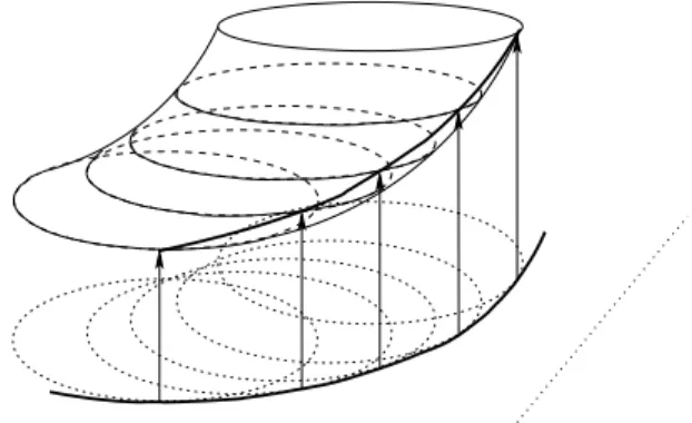
We are given three centres in the (real) plane, and around each of them a concentric family of ncircles — a so calledcircle grid We call a pointP a triple point if each of the three circle families has a member passing through P. Erd˝os, Lov´asz and Vesztergombi [51] asked the following question. For which centre configurations is it possible for infinitely many values of n to choose the circles so that there be at least cn² triple points? Gy¨orgy Elekes [39] have found such examples. On the other hand, in Theorem 1.5.3 we show that for most centre configurations there are no such families of circles.

Theorem 20. There is an absolute constantη >0and a boundn₁∈Zwith the following property. If n > n₁ and three families of concentric circles as above have at least n²⁻^η triple points then the three centres of the families are collinear.

These are the basic ideas of the proof. First we reformulate the problem. Three circles meet in a common point if and only if their radii satisfy a certain polynomial equation. So we have to decide whether the zero locus of this equation, which is an algebraic surface V ⊂R³, is rich or not. This surface V is rich if and only if its equation satisfies a certain partial differential equation constructed with the help of Theorem 14. Finally, checking that partial differential equation is a matter of some algebraic juggling.

Instead of circles we may study more general continuous curves. In place of the n concentric circles we select nmembers from a “continuously parametrised family of continuous curves”. For simplicity here we restrict ourselves to families of curves that can be defined as level-curves of a polynomial function — an “algebraic family of curves” can always be written as a union of such families.

Definition 21. Let G ⊆R² be an open subset in the plane, G denote its closure.

(a) An algebraic family of curves in G is a collection Γ = {γ^(t) ⊂ G : t ∈ [0,1]} of continuous curves which can be defined via a 3-variable polynomialp as follows.

γ^(t)=

(x, y)∈G

p(x, y, t) = 0 .

Note that the polynomial pis not unique.²⁶ The degree of the family Γ is the smallest possible value of deg(p).

(b) The family Γ isexplicitly parametrised, if there is a single member of Γ passing through each point of G, and the implicit function defined by the equationp x, y, f(x, y)

= 0 is analytic in Gand continuous onG.

(c) A continuous curve E ⊂ G is an envelope for the family Γ if it has a tangent line at each of its points, it has no common arc with any member of the family Γ, and for each point P ∈ E there is a member γ^(t) ∈ Γ that is tangent toE at the point P.

26For example all powers ofpdefine the same family Γ.

(21)

5. APPLICATIONS IN GROUP THEORY 17

Let α^(r),β^(s),γ^(t) be algebraic families of curves in the plane. The loci in R³ of the triples (r₀, s₀, t₀) for which the curves α^(r⁰⁾, β^(s⁰⁾, γ^(t⁰⁾ pass through a common point is an algebraic surface V ⊂R³.

Definition 22. We choosencurves from each of the three families. Atriple point of this configuration is a point P in the plane such that each of the three families have a chosen curve passing through P.

If the surface V is not rich (this is the typical situation) then the argument after Theorem 20 implies that there are at mostn^2−η triple points. We cannot decide in full generality whether V is rich or not, but with the help of Theorem 14 we may get useful geometric criteria. The following theorem is a simplified version of Theorem 4.4.1.

Theorem 23. Let G ⊂ H be open subsets in the plane, Γ₁,Γ₂ explicitly parametrised algebraic families of curves in H, and Γ₃ an explicitly parametrised algebraic family of curves of in G, Let d denote the largest among the degrees of the three families. Assume that Γ₃ has an envelope E which belongs to H, and E has no common arc with any member of the the other two families. If we pick n curves from each families (n is sufficiently large) then this configuration has at most n²⁻^η(d) triple points in G, where the constant η(d)>0 depends ond only.

An immediate corollary is Theorem 4.5.1, which had been conjectured earlier by László Székely (see [42, Conjecture 3.41]).

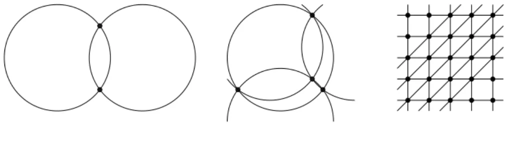
Corollary 24. We are given three points in the plane. We draw n unit circles through each of them. Ifnis large enough then this configutation has at most n²⁻^η triple points. Here η >0 is an absolute constant.

Finally we discuss the following variation on a classical theme (the so- called Orchard problem, see [83, 152]).

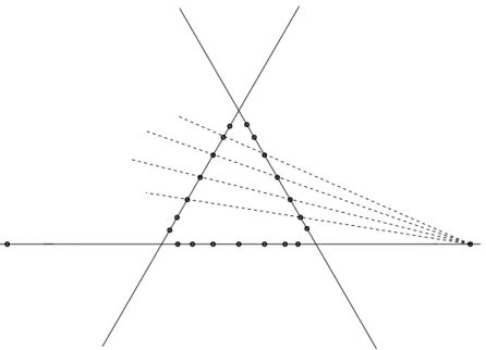
Problem 25. Fix a constantC >0, and find all such subsetsHofnpoints in the plane for which there are at leastCn² lines intersectingHin three or more points.

Our general philosophy suggests that the subset H should be closely related to some kind of “symmetry group”, and indeed, all known construc- tions can be described using groups. However, at the moment we cannot yet find the group in this generality. In Theorem 5.2.2 we solve the problem in a special case that can be handled using algebraic geometry.

Theorem 26. Let H be a finite set of points in the plane such that there are at least c|H|² lines passing through three or more points of H. Assume that an algebraic curve of degree at most d contains all points ofH. If |H|

is large enough (in terms of cand d) then the curve must have degree three.

It is worth noting here that Green–Tao [66] have given sharp upper bound, valid in full generality, on the size of H.

5. Applications in group theory

Conjecture of Babai. Babai [7] conjectured, that all Cayley graphs of all non-abelian finite simple groupsLhave diameter at mostC log|L|c

,

(22)

18 OVERVIEW

where c and C are absolute constants (see Conjecture 2.1.1). The Product theorem (see Theorem 16) implies immediately that the conjecture of Babai holds for finite simple groups of bounded rank.

Corollary 27. If L is a non-abelian finite simple group of bounded rank,²⁷ andα is a symmetric generating set inL, then the Cayley graphΓ(L, α)has diameter at most C log|L|c

, where c and C are absolute constants.

Product decompositions. Let α be a subset of some group. The conjugates of α are the subsets of the form

g⁻¹αg = g⁻¹ag

a∈α

wheregis an arbitrary element of the group. The starting point of Chapter 7 is the following conjecture of Liebeck, Nikolov and Shalev [99].

Conjecture 28. Let G be a non-abelian finite simple group and α ⊆ G a subset of at least two elements. Then G can be written as the product of at most clog|G|/log|α|conjugates of α, where c is a universal constant.

Note that this bound (if true) is optimal, since the number of, say,

1

2log|G|/log|α| term products of elements from α cannot be more than p|G|. Conjecture 28 is the extension of a deep (and useful) theorem of Liebeck and Shalev [104]. They have shown that Conjecture 28 holds in the case when α is a conjugacy class.

If we bound the rank of the groupGthat appears in Conjecture 28 then, combining Theorem 16 with a surprising combinatorial argument, we may handle arbitrary subsets α. This is the content of Theorem 7.1.3.

Theorem 29. Let G be a non-abelian finite simple group of rank²⁷ r and α ⊆ G a subset of at least two elements. Then G can be written as the product of at most c(r) log|G|/log|α| conjugates of α, where the constant c(r) depends onr only.

Theorem 7.1.4 transforms this result into a theorem on growth.

Theorem 30. Let G be a non-abelian finite simple group of rank²⁷ r and α ⊆G an arbitrary subset. Then either there is a conjugate α^′ of the set α such that |αα^′| ≥ |α|^1+ε, where ε(r)>0 is a constant depending on r only, or else α³ =G.

By analogy we transform Conjecture 28 into a conjecture about growth.

In Section 7.6 and Section 7.4 we generalise the classical Pl¨unecke–Ruzsa type inequalities for arbitrary (not necessarily commutative) groups, and with the help of these new inequalities we prove that the original Conjec- ture 28 implies our new conjecture concerning growth.

Conjecture 31. There is a real constant ε > 0 and an integer constant b > 0 with the following property. In each finite simple group G for all subsets α either there is a conjugate α^′ such that |αα^′| ≥ |α|^1+ε, or G is equal to the product of b conjugates ofα.

It is possible that Conjecture 31 holds with b = 3. On the other hand, there are counterexamples to b= 2.

27Therank of a finite simple groupGis roughly equal to the smallest valuen such thatGis isomorphic to a subgroup ofSL(n, q) for some prime powerq.

(23)

5. APPLICATIONS IN GROUP THEORY 19

Permutation groups. A graph Γ is said to beG-vertex-transitiveifG is a subgroup of Aut(Γ) acting transitively on the vertex set of Γ. We say that a G-vertex-transitive graph Γ isG-locally primitive if the stabiliser G_α of the vertex αinduces a primitive permutation group on the set of vertices adjacent to α. (Because of the transitivity this holds either for all vertices, or for none of them.) In 1978 Richard Weiss [170] conjectured that, for a finite connected G-vertex-transitive,G-locally primitive graph Γ, the size of G_α is bounded above by some function depending only on the valency of α. (By the transitivity, all vertices have equal valencies, and the stabiliser subgroups are all isomorphic to each other.)

In Chapter 6 we study the Weiss conjecture. The reduction theorems in [129, 126] show that it is enough to bound the size of the H_α stabiliser subgroups in certain H-vertex-transitive graphs, where H is a composition factor of the group G. As H is a simple group, we may use the Product theorem (see Theorem 16) for studying theH-vertex-transitive graphs. With this method we are able to deduce the Weiss conjecture in the case when the composition factors of Ghave bounded rank.

Definition 32. Define BCP(r) to be the class of finite groups G which have no section H/K, where K < H ≤ G and K is normal in H, that is isomorphic to the alternating group Alt(r+ 1).²⁸

The class of BCP(r)-groups was first considered by Babai, Cameron and P´alfy [4]. They showed that primitive BCP(r)-groups of degree nhave order at mostn^f(r). This result is an essential ingredient of many polynomial time algorithms for permutation groups related to the graph isomorphism problem [86]. The BCP(r)-groups play also a very important role in the theory of subgroup growth of residually finite groups (see [107]).

Theorem 6.1.2 states that the Weiss conjecture holds in the class of BCP(r) groups. The full Weiss conjecture asks then whether the functiong below can be chosen not to depend on r.

Theorem 33. There exists a function g : N×N → N such that, for Γ a connected G-vertex-transitive, G-locally primitive graph of valency at most d, if G is a BCP(r)-group, then a vertex stabiliser in G has size at most g(r, d).

28It is easy to see that all composition factors of a BCP(r)-group must be either a sporadic simple group, or a finite simple group of rank at mostr.

(24)

(25)

CHAPTER 1

How to find groups

1.1. Introduction

This chapter is essentially equivalent to our joint paper [48] with Gy¨orgy Elekes. The germs of the paper were two earlier manuscripts: “How to find groups?” by myself and our joint work “Triple points of circle grids”. They have been circulated as sort of “technical reports” for several years. We decided to publish the method based upon the two of them as one article, since it is the interaction of the two points of view that makes the ideas work.

The philosophy of our main results (and also of their applications) is a general principle of geometry: whenever we find a lot of unexpected coincidences, then somewhere in the background there lurks a large group of symmetries. There are infinitely many variations on this theme, both continuous and discrete, and we shall only touch a few of them. We focus on algebraic geometry, with applications to Erd˝os geometry. To state precise results, we have to measure the amount of coincidences a certain geometric configuration has. In the discrete case we can simply count them while in the continuous case we measure the dimension of the parameter space instead.

As for the discrete versions, we shall usually consider finite Cartesian productsX×Y×Z ={(x, y, z)

x∈X, y∈Y, z∈Z}, where, in the simplest case, X, Y, Z ⊂C, or in a more general setting, for some varieties A, B, C, we have X⊂A,Y ⊂B,Z ⊂C, and thusX×Y ×Z ⊂A×B×C. (In what follows, n will denote a large positive integer, usuallyn=|X|=|Y|=|Z|. Moreover, there also appear some constants like c > 0 or natural numbers d, k, r which remain fixed while n→ ∞.)

Geometric questions which involve Euclidean distances often lead to polynomial relations of type F(x, y, z) = 0 for some F ∈ R[x, y, z]. Sev- eral problems of Combinatorial Geometry can be reduced to studying such polynomials which have many zeroes onn×n×nCartesian products. The special case when the relation F = 0 can be re–written as z =f(x, y), for a polynomial or rational function f ∈R(x, y), was considered in [45]. Our main goal is to extend the results found there to full generality (and also to show some geometric applications, e.g. one on ”circle grids”).

The main result of Chapter 1 concerns low–degree algebraic setsF which contain “too many” points of a (large) n×n×n Cartesian product. Then we can conclude that, in a neighborhood of almost any point, the setF must have a very special (and very simple) form. Roughly speaking, then eitherF is a cylinder over some curve, or we find a group behind the scene: F must

21

(26)

22 1. HOW TO FIND GROUPS

be the image of the graph of the multiplication function of an appropriate algebraic group (see Theorem 1.1.3 for the 3D special case and Theorem 1.4.2 in full generality).

The structure of Chapter 1. We first state Theorem 1.1.3, the three dimensional special case of our Main Theorem 1.4.2. Its proof – as well as its arbitrary dimensional version — can be found in Section 1.4. It relies upon two basic tools: incidence bounds and composition sets. The former are described in Section 1.2 while the latter are the subject of Section 1.3.

Moreover, in Section 1.5, we give an immediate consequence of our incidence bounds which concerns a problem posed by Hirzebruch and was partially solved in [110]. Also an application of our three dimensional Theorem 1.1.3 can be found there.

The main result inC³ (and R³). In [45] those bivariate polynomials F ∈R[x, y] were characterized whose graph (inR³) passes through at least cn² points of an n×n×n Cartesian product X×Y ×Z ⊂ R³, where n = |X| = |Y| = |Z|. It was shown there that F must be very special, provided that n > n₀=n₀(c,deg(F)). More precisely,

F(x, y) =

(f g(x) +h(y)

; or f g(x)·h(y)

,

and these types of polynomials really have graphs which are incident upon many points of appropriately chosen Cartesian products, e.g., if both g(X) and h(Y) are arithmetic/geometric progressions. (The reader may have observed the additive grouphR,+iand the multiplicative grouphR\ {0},·i in the background.)

We generalise the foregoing result several ways:

(a) instead of real variables, we consider complex ones;

(b) instead of graphs of bivariate polynomials, we allow algebraic varieties (surfaces) inC³;

(c) instead ofcn² points, we only require that the surface in question passes through as few asn²⁻^η points of a Cartesian product, for a sufficiently small positiveη.

To state the Theorem in its simplest (lowest interesting dimensional) 3D form, we recall the notion of “connected one dimensional algebraic groups”.

A good reference for the list below: Excersise 11, 12, 13 in Chapter 1 §2 of [117]. In this case, the complex analytic structure completely determines the algebraic structure, so we describe these groups as analytic manifolds. The following three types of groups are calledcomplex connected one dimensional algebraic groups:

(a) hC,+i;

(b) hC\ {0},·i ∼=hC,+i/Z;

(c) hC,+i/L, where L is a parallelogram lattice (an affine image of Z²).

Algebraically these occur e.g. as the usual groups on cubic curves in the plane.

The irreducible real one dimensional algebraic groups are appropriate subgroups of those above. Analytically they are all isomorphic to the real line

(27)

1.1. INTRODUCTION 23

hR,+i, to the unit circle hS¹,·i in the complex plane, or two copies of the unit circle Z₂⊕ hS¹,·i. However, in contrast to the complex case, several nonequivalent algebraic structures correspond to the same analytic group.

Example 1.1.1. If hG,⊕i is any of the foregoing — real or complex — algebraic groups (or even if it is a higher dimensional one) then it is easy to show examples of n×n×n Cartesian productsX×Y ×Z inG³ or inC³, and two dimensional subvarieties (surfaces) which contain ≈n²/8 points of X×Y ×Z, as follows.

(a) Without loss of generality, assume that n is odd, say n = 2k+ 1, and pick an arbitrary non-torsion element a∈ G (i.e. one of infinite order).

Let

X=Y =Z :={−ka,−(k−1)a, . . . ,−a,0, a, . . . ,(k−1)a, ka} and define

Gsp :=

(x, y, z)

x⊕y⊕z= 0∈ G ,

which we call the special subvariety in G³. (Of course, in higher dimensional — usually non–Abelian — groups the multiplicative notation would be more appropriate.) It is easy to check that this Gsp will, indeed, contain≥ ⌈k²/2⌉ ≈n²/8 points ofX×Y ×Z. Moreover, ifU ⊂ G is any neighborhood of 0, then we can choose X = Y = Z ⊂ U via choosing anasufficiently close to 0.

(b) In (a) we have found a Cartesian product set in any neighborhood of (0,0,0) ∈ G³. We can improve on this: there are similar Cartesian product sets in any neighborhood of any point (a, b, c)∈ Gsp. Indeed, if a⊕b⊕c= 0 then we may define X^′ =X⊕a, Y^′ =b⊕c⊕Y ⊕a⊕b and Z^′ = c⊕Z (these formulas work even if G is noncommutative).

Again, Gsp contains a quadratic order of magnitude of points of the Cartesian product X^′×Y^′×Z^′, but this Cartesian product lives in the neighborhood of (a, b, c).

(c) More generally, suppose we have a connected open set of the form U = U_f ×Ug×U_h ⊆ G³ intersecting the subvariety Gsp of (a), nonconstant analytic functions f :U_f →C, g :U_g → C, h:U_h → C, and a surface V ⊂C³ containing the f×g×h-image ofGsp∩U:

V ⊇n

f(x), g(y), h(z)

∈C³

(x, y, z)∈U, x⊕y⊕z= 0∈ Go . We may assume, that the functions f, g, h are one-to-one, otherwise we replace their domain with appropriate subsets. Then we choose a Cartesian product X^′ ×Y^′ ×Z^′ ⊂ U as in (b). Then V contains a quadratic order of magnitude of points of the Cartesian productf(X^′)× g(Y^′)×h(Z^′).

Definition 1.1.2. Let U, V be open subsets in C or in a connected one- dimensional algebraic group G. A multi-valued function f : U → V is an analytic multi–function if, except for a finite point set H ⊂ U, every P ∈U\H has a neighborhood wheref is the union of finitely many one-to- one analytic functions, called the analytic branches off nearP, andf has no values at points of H. The complexity of such a function is the larger