Polynomial approximation for fast generation of associated Legendre functions

https://doi.org/10.1007/s40328-018-0216-1 ORIGINAL STUDY

Polynomial approximation for fast generation of associated Legendre functions

M. R. Seif¹ · M. A. Sharifi^2,3 · M. Eshagh⁴

Received: 16 June 2017 / Accepted: 15 April 2018 / Published online: 28 April 2018

© Akadémiai Kiadó 2018

Abstract Today high-speed computers have simplified many computational problems, but fast techniques and algorithms are still relevant. In this study, the Hermitian polynomial approximation is used for fast evaluation of the associated Legendre functions (ALFs). It has lots of applications in geodesy and geophysics. This method approximates the ALFs instead of computing them by recursive formulae and generate them several times faster.

The approximated ALFs by the Newtonian polynomials are compared with Hermitian ones and their differences are discussed. Here, this approach is applied for computing a global geoid model point-wise from EGM08 to degree and order 2160 and in propagat- ing the orbit of a low Earth orbiting satellite. Our numerical results show that the CPU- time decreases at least two times for orbit propagation, and five times for geoid computa- tion comparing to the case where recursive formulae for generation of ALFs are used. The approximation error in the orbit computation is at a sub-millimeter level over two weeks and that the computed geoid 0.01 mm, with a maximum of 1 mm.

Keywords Associated Legendre function · Polynomial approximation · Newton polynomial · Hermite polynomial · Fast orbit propagation · Geoid computation

* M. R. Seif m.r.seif@ut.ac.ir

1 Department of Surveying Engineering, Arak University of Technology, Arak, Iran

2 School of Surveying and Geospatial Engineering, College of Engineering, University of Tehran, Tehran, Iran

3 Research Institute of Geoinformation Technology (RIGT), College of Engineering, University of Tehran, Tehran, Iran

4 Department of Engineering Science, University West, Trollhaättan, Sweden

1 Introduction

The associated Legendre functions (ALFs), are the fundamental mathematical tools in var- ious fields of science , which are applied in geoscience (Hofmann-Wellenhof and Moritz 2006; Kaula 2000; Fukushima 2012), satellite orbit determination (Montenbruck and Gill 2000) and other scientific fields such as atomics and molecular physics (Haken and Wolf 2004), and electro-magnetics (Rothwell and Cloud 2001). Some well-known recursion for- mulas (Hofmann-Wellenhof and Moritz 2006) are normally used for generating the ALFs (see e.g. Abramowitz and Stegun 1972; Bettadpur et  al. 1992; Ilk 1983; Lundberg and Schutz 1988; Hobson 1955; Gautschi 1967), which are classified into three categories of degree-alone, order-alone and degree-order recursions. Holmes and Featherstone (2002) categorize them into standard forward column and row, Belikov column and recursion between every other order and degree.

The most limiting issue of these methods is their low computation speed especially when the ALFs are generated to high degrees and orders. However, the approximation methods could be used to speed up the computations significantly. Since the ALFs are of polynomial nature, then a low-order polynomial can be used to approximate them (Phillips 2003; Hoffman and Frankel 2001). The Newtonian polynomial is one of these methods, which approximates the values of ALFs at some specific points and uses the function val- ues. Alternatively, the Hermitian polynomials, which uses the values of ALFs as well as its derivatives up to a certain order (Yang et al. 2005), can be applied for approximating the ALFs. This method uses more information about the function than the former and is expected to deliver more precise values for the ALFs.

The global gravity field models are presented in terms of spherical harmonic coeffi- cients, and therefore, for generating the gravity-dependent quantities from them, their spherical harmonic expansion, involving the ALFs, should be used. Consequently, fast computational performance of such harmonic series depends on the synthesis method and fast generating of ALFs. The Fourier transform is an option for such a goal over regular grids (Földváry 2015; Sneeuw and Bun 1996; Cheong et al. 2012).

Vectorization is another alternative based on array programming to speed up code, espe- cially for interpreted languages like Matlab. The vectorization (Eshagh 2009; Sharifi 2006) is commonly-used for generating of the geoid and/or other anomalous quantities. Normally, for generating these quantities over an area 4 loops are used, however, by vectorization and using matrix algebraic processes the number of the loops can be reduced. The vectorization can be done on the expansion so that by a simple matrix product the necessary quanti- ties are generated by two loops. In addition, one more loop can be eliminated. Eshagh and Abdollahzadeh (2010) called this method semi-vectorization. However, this method is effi- cient if all quantities are computed at surface of a sphere and in regular grid forms. There- fore, if the geocentric distances of the computation points vary from one point to another, irregular semi-vectorization can be used (Eshagh and Abdollahzadeh 2012).

In the cases of having irregular points there are two options, vectorization over degree- order of the spherical harmonic expansion and use two loops to vary the positions, or to generate a dense grid of the quantities and thereafter determine the values at the points by interpolation techniques. The former is rather time-consuming and the latter contaminates the interpolation errors to the results.

The former method can be applied to generate the acceleration vectors of the gravity field (Seeber 2003) at satellite altitudes for orbit determination. Vectorization is only pos- sible in such a problem over the degree and order of the spherical harmonics and not the

satellite orbit. Then, parallel computation could not be carried out as the satellite state vec- tor is propagated step-by-step using numerical integration. This make the problem time- consuming even if with advanced and fast computers.

Hwang and Lin (1998) presented a method for such a purpose and tried to first find the maximum effective degree of the spherical harmonic expansion to avoid generating unnec- essary high degrees and orders ALFs. In this paper, our idea is to approximate the ALFs using the Newton and Hermitian methods to approximate the ALFs instead of using their recursion formulae. Although, the Hermite polynomial could be fitted to data more accu- rately, the saved grid data will be lower for Newton method in comparison with Hermite.

Because the Newton polynomial needs only function value for the function estimation.

Therefor, the Newton interpolation could be recommended for cases that the high accuracy is not very critical.

The represented idea is very advantageous especially when the satellite orbit have to be propagated repeatedly, for example, in designing satellite constellations using optimiza- tion algorithm. Here, the mathematical methods of synthesizing spherical harmonics using these approaches are discussed and later the idea is applied for orbit integration of a low Earth orbiter and to computed global high-resolution geoid model using EGM08.

2 ALFs approximation using the Newton interpolation

The Newton interpolation approach is famous due to its simple principle (Atkinson 2008).

In this method, a ( n−1)-degree polynomial is fitted to a set of function values in a grid of points. The n-points Newton interpolation is formulated in a simplified form for equidistant sampling points with step-size h which are denoted by x_i=x₀+i h for i=0, 1,…, n−1 , ( x₀ is the start point). By defining the notation x=x₀+s h , the difference x−x₀ can be written as s h . So the Newton polynomial could be expressed as (Hildebrand 1987):

where (s i

) is the binomial coefficient, and Δⁱf(x₀) is the forward differences of f(x₀) defined recursively by:

In order to approximate the ALFs, f(x_i) are ALF matrices in the equidistant grid points of latitude denoted by 𝐏(𝜑_i) . Then, a matrix of n-degree Newton interpolators is fitted to ( n+1 ) given data points, {𝜑_i,𝐏(𝜑_i)}ⁱ⁼ⁿ_i=0.

This matrix is square with L+1 rows and columns, where L is the maximum degree and order of the ALFs. The element in the (i+1)-th row and (j+1)-th column of the matrix is the interpolating polynomial that approximate the ALFs of degree i and order j. For exam- ple, the approximated ALFs matrix using fifth–degree Newton polynomial in the latitude 𝜑 has been formulated as

(1) N(x) =

∑n−1 i=0

(s i )

Δⁱf(x₀)

Δ⁽⁰⁾f(x₀) ∶=f(x₀) (2)

Δ^(k)f(x₀) ∶= Δ^(k−1)f(x₁) − Δ^(k−1)f(x₀), k≥1.

(3) 𝐏_N(𝜑) =

∑5 i=0

(𝜎 i )

Δⁱ𝐏(𝜑₀)

where 𝜎= (𝜑 − 𝜑₀)∕Δ𝜑 with the length of interval Δ𝜑 = 𝜑₁− 𝜑₀, and the needed forward differences are:

where 𝐏(𝜑_i) are the ALFs matrices with L rows and columns in the nearest points of the grid to the desired latitude denoted by 𝜑₀,𝜑₁,…,𝜑₅ . By substituting Eq. (4) into Eq. (3) and after doing some simplifications, we obtain the fifth-degree Newton polynomial:

Although the polynomial interpolation has many advantageous applications, it suffers from a serious weakness. The low-degree polynomials could not exactly fit to the data set, and increasing the polynomial degree causes a larger approximation error. Although the higher degree polynomials could precisely resample function values in the sampling points, it could not guarantee better fitting result in the midpoint due to the polynomial oscillation (Yang et al. 2005; Szegö 1975). In other words, low-degree polynomials tend to be smooth and the high-degree ones tend to be lumpy (Kolb 1984). As an idea, the Hermite polyno- mial could be used to reduce such oscillation (Boyd and Alfaro 2013). Generally, an inter- polation function is called Hermitian, if it satisfies interpolating conditions on the deriva- tives (Szegö 1975) as well. The Hermitian interpolation is described in following section.

3 ALFs approximation using the Hermitian interpolation

In order to achieve high precision in interpolation, an interpolating polynomial is derived so that it passes through the points meanwhile considering the low-order derivatives of the func- tion up to given orders. This polynomial is called the Hermitian (Yang et al. 2005). Unlike other interpolation methods, it forces the polynomial to match the function values and its derivatives at sampling points (Embree 2010). The n-points cubic Hermite interpolation poly- nomial can be set up as:

Δ⁽⁰⁾𝐏(𝜑₀) ∶= 𝐏(𝜑₀) (4)

Δ^(k)𝐏(𝜑₀) ∶= Δ^(k−1)𝐏(𝜑₁) − Δ^(k−1)𝐏(𝜑₀), k≥1.

(5) 𝐏̃_N(𝜎) = 1

120

(120−274𝜎+255𝜎²−85𝜎³+15𝜎⁴− 𝜎⁵) 𝐏(𝜑₀) + 1

120

(600𝜎−770𝜎²+355𝜎³−70𝜎⁴+5𝜎⁵) 𝐏(𝜑₁) + 1

120

(−600𝜎+1070𝜎²−590𝜎³+130𝜎⁴−10𝜎⁵) 𝐏(𝜑₂) + 1

120

(400𝜎−780𝜎²+490𝜎³−120𝜎⁴+10𝜎⁵) 𝐏(𝜑₃) + 1

120

(−150𝜎+305𝜎²−205𝜎³+55𝜎⁴−5𝜎⁵) 𝐏(𝜑₄) + 1

120

(24𝜎−50𝜎²+35𝜎³−10𝜎⁴+1𝜎⁵) 𝐏(𝜑₅)

(6) H(x) =

∑n−1 i=0

(𝛼_i(x)f(x_i) +h𝛽_i(x) ̇f(x_i) +h²𝛾_i(x)̈f(x_i))

where f_i,ḟ_i and f̈_i denote, respectively, the value of function , and its first- and second-order derivatives on the grid points x_i within the range [x₀, x_n−1]. In order to simplify further, let us reformulate Eq. (6) based on the normalised distance from x₀ i.e. 𝜎= (x−x₀)∕h, h denotes the grid step-size, as

(3n−1)-degree polynomials {𝛼_i,𝛽_i,𝛾_i}ⁿ⁻¹_i=0 are constructed so that they satisfy the following constraints

where 𝛿_i,j is Kronecker delta. In accordance with standard literature, the prime and double- prime denote the first and second derivative of polynomials {𝛼_i,𝛽_i,𝛾_i} with respect to the argument 𝜎, respectively. These constraints are satisfied by the following equations that are the basis functions for the expansion Eq. (7)

In Eq. (9), 𝓁_i(𝜎) is the Lagrange basis polynomial (Szegö 1975)

It is should be noticed that for n grid points, the degree of 𝓁

i is (n−1). As an example, we develop Eq. (7) that matches function and its first- and second-derivatives. The ALFs approximation using the 2-points Hermitian polynomial can be formulated as:

where local variable 𝜎= (𝜑 − 𝜑₀)∕(𝜑₁− 𝜑₀). The polynomials {𝛼_i,𝛽_i,𝛾_i}¹_i=0 needed in Eq.

(11) are functions of the Lagrange polynomial 𝓁

i(𝜎) and its first and second derivatives:

These polynomials have been listed in Table 1.

By substituting the listed polynomials into Eq. (11) and after some simplification, we have

(7) H(𝜎) =

∑n−1 i=0

(𝛼_i(𝜎)f(𝜎_i) + 𝛽_i(𝜎) ̇f(𝜎_i) + 𝛾_i(𝜎)̈f(𝜎_i)) .

(8) 𝛼_i(𝜎_j) = 𝛿_i,j,𝛽_i(𝜎_j) =0, 𝛾_i(𝜎_j) =0,

𝛼_i^�(𝜎_j) =0, 𝛽_i^�(𝜎_j) = 𝛿_i,j, 𝛾_i^�(𝜎_j) =0, 𝛼_i^��(𝜎_j) =0, 𝛽_i^��(𝜎_j) =0, 𝛾_i^��(𝜎_j) = 𝛿_i,j.

(9) 𝛼_i(𝜎) =

[ 1−3𝓁^�

i(𝜎_i)(𝜎 − 𝜎_i) + (12𝓁^�

i

2(𝜎_i) −3𝓁^��

i(𝜎_i) 2

) (𝜎 − 𝜎_i)²

] 𝓁³

i(𝜎), 𝛽_i(𝜎) =[

(𝜎 − 𝜎_i) −3(𝜎 − 𝜎_i)²𝓁^�

i(𝜎_i)] 𝓁³

i(𝜎), 𝛾_i(𝜎) =1

2(𝜎 − 𝜎_i)²𝓁³

i(𝜎).

(10) 𝓁i(𝜎) =

∏n−1 j=0,j≠i

(𝜎 − 𝜎_j) (𝜎_i− 𝜎_j).

(11) 𝐏̃_H(𝜎) =

∑1 i=0

(𝛼_i(𝜎)𝐏(𝜎_i) + 𝛽_i(𝜎) ̇𝐏(𝜎_i) + 𝛾_i(𝜎) ̈𝐏(𝜎_i))

𝓁 (12)

0(𝜎) = −(𝜎 −1), 𝓁₁(𝜎) = 𝜎.

where 𝜎_i= (𝜑_i− 𝜑₀)∕h . 𝐏, ̇𝐏 and 𝐏̈ denote respectively the matrices of zero-, first- and second-order derivatives of ALFs with respect to 𝜎= (𝜑 − 𝜑₀)∕h:

The accuracy and computation time of these polynomial approximations are compared in the following section of the numerical analysis.

4 Numerical analysis

As described, the ALFs are not evaluated using the recursive formula, but approximated by low-degree polynomials to speed up the computation. To do this, we need a set of function values (with or without derivatives) on a grid points, better to be equidistant. Here, grids of the ALFs matrices and their first- and second-order derivatives are produced. The latitude interval of the grid was considered 0.5^◦ in 𝜑∈ [0^◦, 90^◦] for the accuracy analysis and the satellite orbit propagation. This interval is suffices as the ALFs for the southern hemisphere can be computed from those of northern by:

where P̄_lm is the fully normalised ALFs of degree l and order m. Therefore, for the southern latitude, they are approximated by their symmetric latitude, in northern latitude, and finally converted to the southern one.

In this section, we examine the approximation error of the ALFs of different orders and degrees using the lower degree polynomial, Newtonian and Hermitian polynomials of degree five. At the next steps, different degrees of the approximating polynomials will be investigated. Since the behaviour of the ALFs and consequently the approximation accu- racy is latitude-dependent, they should be checked at various latitudes. Here, three latitude

(13) 𝐏̃

H(𝜎) =(

1−10𝜎³+15𝜎⁴−6𝜎⁵) 𝐏(𝜎₀) +(

10𝜎³−15𝜎⁴+6𝜎⁵) 𝐏(𝜎₁) +(

𝜎−6𝜎³+8𝜎⁴−3𝜎⁵)

̇𝐏(𝜎₀) +(

−4𝜎³+7𝜎⁴−3𝜎⁵)

̇𝐏(𝜎₁) +(

1∕2𝜎²−3∕2𝜎³+3∕2𝜎⁴−1∕2𝜎⁵)𝐏̈(𝜎₀) +(

1∕2𝜎³− 𝜎⁴+1∕2𝜎⁵)𝐏̈(𝜎₁)

(14)

̇𝐏(𝜎) =𝜕𝐏

𝜕𝜎 =𝜕𝐏

𝜕𝜑

𝜕𝜑

𝜕𝜎 =h𝜕𝐏(𝜑)

𝜕𝜑 𝐏̈(𝜎) =𝜕 ̇𝐏

𝜕𝜎 =𝜕 ̇𝐏

𝜕𝜑

𝜕𝜑

𝜕𝜎 =h²𝜕²𝐏(𝜑)

𝜕𝜑²

(15) P̄_lm(sin(−𝜑)) = ̄P_lm(−sin(𝜑)) = (−1)^l−mP̄_lm(sin(𝜑))

Table 1 The polynomial required for Hermite

interpolation between two points

𝛼i 𝛽i 𝛾i

i=0 (1+3𝜎+6𝜎²)(1− 𝜎)³ (𝜎 +3𝜎²)(1− 𝜎)^{3 1}

2𝜎²(𝜎 −1)³ i=1 (10−15𝜎+6𝜎²)𝜎³ [(𝜎 −1) −3(𝜎 −1)²]𝜎^{3 1}

2(𝜎 −1)²𝜎³

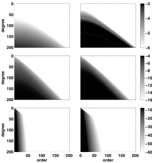
at the equator 𝜑₁=0.25^◦ , mid-latitude 𝜑₂=45.25^◦ and near pole locations 𝜑₃=89.75^◦ are considered and the approximation errors the Hermitian and Newtonian polynomials are presented in Fig. 1 for different degrees and orders. Since the mid-point of any sub-interval typically has the largest approximation error, these latitudes have the largest approximation errors at the equator, mid-latitude and the North Pole. Then, they are proper check points for testing the quality of approximation.

In Fig. 1, the horizontal and vertical axes show, respectively, the orders and degrees of the ALFs matrix and darker cells displays larger value of the approximation error. The figure shows that the error of Newtonian (right sub-figures) and Hermitian polynomial (left panels) at 𝜑₁=0.25^◦, 𝜑₂=45.25^◦ and 𝜑₃=89.75^◦ from top to bottom, respectively. As seen, generally, the Hermitian method is more precise than the Newtonian one. The Hermi- tian polynomial uses the function values as well as its first- and second- derivatives, which

degree

0 50 100 150 200

degree

0 50 100 150 200

order

degree

50 100 150 200 0

50 100 150 200

order

0 50 100 150 200 −60

−50

−40

−30

−20

−10

−16

−14

−12

−10

−8

−6

−4

−6

−5

−4

−3

Fig. 1 The absolute error of the ALFs approximation in logarithm scale, right-(top, middle and bottom) using the Newton polynomial of degree 6 and left-(top, middle and bottom) using the Hermitian polyno- mial respectively in 𝜑₁=0.25^◦,𝜑₂=45.25^◦, and𝜑₃=89.75^◦ (Note: the scale bar is similar for two sub- figures in each row)

are related to the slope and curvatures of the interpolating polynomial. They are entered to the interpolating procedure as constraints. Then, we can expect that it provide better results than the Newtonian one.

Another issue is that the error pattern is a function of the degree and order of ALFs. As we know, an l-th degree and m-th order of the ALFs has l−m distinct roots, i.e. (l−m) zeros all in the interval (−1, 1) . More roots mean more oscillations of the ALFs, and it could increase the polynomial approximation error. As the number of the roots of ALFs, l−m roots, decreases for higher order, the approximation error in the higher orders for all degrees is substantially reduced. On the other hand, by similar reasoning, it could be concluded that the approximation error in the higher degrees for all order is substantially increased. The maximum error of the ALFs approximation error occurs in the higher degree of the zonal terms.

Furthermore, a considerable decrease of the approximation error in the polar regions for both methods is seen. It is due to the near zero value and smooth behaviour of the ALFs in polar region for m≠0 . The approximation error decreases commensurately as the func- tion becomes smoother. In order to investigate the dependency of the approximation error on the latitude, the error pattern has been shown for a few degrees and orders of the ALFs as examples. First, the zonal terms m=0 as the ALFs with the maximum latitude-varia- tions, the sectorial terms m=l as the ALFs with the minimum ones, and the tesseral terms m=l∕2 as a middle case.

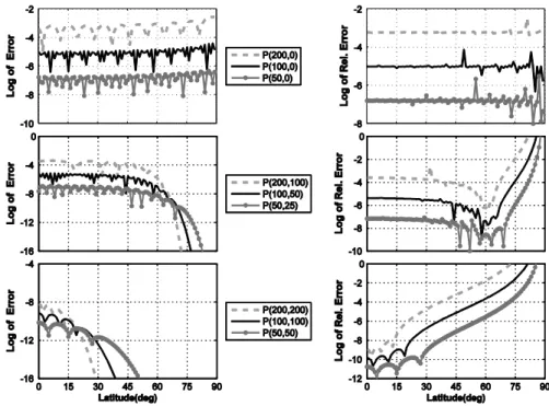
In addition, Fig. 2 displays the absolute and relative errors of a few special degree/order of ALFs versus latitude in the logarithmic scale. The error that is less than 10⁻¹⁶ , about machine error, has been neglected, and Fig. 2 (middle and bottom) is cropped where Loga- rithm of error is − 16.

Fig. 2 The absolute (left) and relative (right) errors of ALFs in degrees,l=200, 100, 50 and orders, m=0 (top), m=l∕2 (middle) and m=l (bottom) for the Hermite method

As illustrated in Fig. 2, the maximum error occurs in the case m=0 . It is in agreement with the previous finding that the maximum error of the ALFs approximation is expected on the zonal terms. In addition, a large reduction in the approximation error is observed for the m=l∕2 and m=l cases at near the Polar latitude, because of the smoothness of the the ALFs over this region.

Some oscillations are seen in the absolute errors which might be related to the periodic variations of the ALFs. In order to check this, the relative error is plotted also in Fig. 2 (right panels) and the lack of periodic variation in the relative error figure confirms this. In this case, the sharp rise near polar region is due to the fact that the ALFs are close to zero in polar region, except the case m=0.

As another test to analyse the ALFs accuracy, the relative accuracy was done based on the orthogonality of the ALFs. The summation, over degree and order, of the square of ALFs is up to L (Holmes and Featherstone 2002)

Figure 3 shows the reduced relative accuracy to evaluate Eq. (16) for the approxi- mated ALFs. The reduced relative accuracy (RRA) truncates the first 12 dig- its of the relative accuracy which are defined by RA minus its average. The average is

−9.59187232334238×10⁻⁵ . Although the changes are significant at the poles (cf. Fig. 2) due to the lower relative accuracy of the sectorial and tesseral terms in high latitudes, the difference between maximum and minimum of the relative accuracy is very low and, about 3.5∗10⁻¹³.

In this part, we are interested in analyzing the effect of the grid size on the ALFs approximation. Figure 4 represents the maximum of the error of ALFs in loga- rithm scale for different grid size. Since the error change for different degree/order of the ALFs, this analysis is repeated for a few cases i.e. L=200, 500, 1000 . As it was (16) Σ_L=

∑L l=0

∑l m=0

P_lm(𝜑)²= (L+1)²

−90 −60 −30 0 30 60 90

−1.5

−1

−0.5 0 0.5 1 1.5 2 2.5x 10⁻¹³

Latitude (degree)

Reduced Relative Accuracy

max−min=3.5*10⁻¹³ mean of RA=−9.5918e−05

Fig. 3 The reduced relative accuracy (relative accuracy minus its mean) to evaluate ∑200 l=0

∑^l

m=0P_lm(𝜑)² for various latitude for Hermite method with grid size of 0.5^◦

predictable, the higher degree/order of the ALFs need more dense grid size for high accuracy approximation.

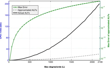
In the next step, we examine the CPU-time reduction by using this approximation.

Figure 5 illustrates the CPU-time needed for evolution of function between the ordinary and approximation methods for different L . This computation is implemented in Matlab 2014 and run in a PC with 16 GB of memory and Core i7 Processor. In addition, Fig. 5 shows the maximum of error of the ALFs approximation (the max differences between the matrices of the approximated and actual ALFs) in logarithm scale.

0.05 0.1 0.15 0.2 0.25 0.3 0.35 0.4 0.45 0.5

10⁻¹⁰ 10⁻⁸ 10⁻⁶ 10⁻⁴ 10⁻² 10⁰

Grid Size (deg)

Log of Maximum Error L=1000

L=500 L=200

Fig. 4 The effect of the grid size on the accuracy of the approximated ALFs

0 500 1000 1500 2000 2190

0 40 80 120 160 200

Max degree/orde (L)

CPU−Time (sec)

10⁻¹⁴ 10⁻¹² 10⁻¹⁰ 10⁻⁸ 10⁻⁶ 10⁻⁴

Max Error of approximated ALFs

Max Error Approximated ALFs Actual ALFs

Fig. 5 The CPU-time needed for 100 evaluations of the actual and approximated ALFs, and maximum error of ALFs versus L ( grid size=0.05^◦)

Based on the results demonstrated in Fig. 5, it is concluded that the CPU-time needed for the ALFs computation increases so as L. Because, (L+1)(l+2)∕2 values of the ALFs have to be computed using the recursive algorithm. Besides, the approximation approach needs more CPU-time to compute ALFs for larger L as the size of matrices in Eq. (13) becomes larger as L increases, and it consumes more time for process of the matrix alge- bra. However, in approximate method the CPU-time is lower than and evaluates the ALFs significantly faster. For L=140 , the speed-up factor is about 4.5. The speed-up factor is defined by the ratio of the CPU-time needed for evaluating the ALFs to one necessary for approximating the ALFs. The factor is about 9 for L=2190 . The proposed method is effective in accelerating the computation even for low L. As an example, the speed-up fac- tor is 2 for L=20.

4.1 Orbit propagation

Besides of the CPU-time and accuracy analysis, we test the efficiency of the proposed algorithm in a real example. As it was described before, the dynamic orbit integration is selected as a case study. In this section, the effect of the approximation errors of the ALFs in the orbit propagation process are studied. The motion of a satellite in a gravitational field of an attractive body is expressed by the equations of motion (Seeber 2003):

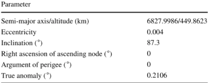
where 𝐚_p stands for the perturbing accelerations acting on the satellite, the gravitational perturbation such as geopotential, gravity of the Sun and Moon and indirect effect of third body, solid and ocean tide, and non-gravitational forces such as atmospheric drag and solar radiation pressure. Amongst the perturbing accelerations, the Earth’s gravity acceleration computation requires the ALFs and it is the main reason of the highly time-consuming process of the satellite orbit propagation. In this paper, the equations of motion of a LEO satellite has been solved in the Earth’s gravity field as a case study. The numerical study is carried out based on the assessment of the accuracy and usability of our approach to accel- erate the satellite orbit propagation process. The accuracy of the fast propagated orbit has been analyzed in this section for a CHAMP-like satellite (Reigber et al. 2002). The orbital elements of the satellite has been listed in Table 2.

The orbits, computed using the approximated and actual accelerations, are respec- tively called approximated and reference orbits. The approximated acceleration is uti- lized the approximated ALFs instead of the actual ones. The accuracy of the approxi- mated orbits obtained from the different polynomial approximation methods have been

(17)

̈𝐫= −GM

r³

𝐫+ 𝐚_p, 𝐫(t₀) = 𝐫₀; ̇𝐫(t₀) = ̇𝐫₀

Table 2 The orbital element of a

CHAMP-like satellite Parameter

Semi-major axis/altitude (km) 6827.9986/449.8623

Eccentricity 0.004

Inclination ( ^◦) 87.3

Right ascension of ascending node ( ^◦) 0

Argument of perigee ( ^◦) 0

True anomaly ( ^◦) 0.2106

compared in this section. Here, the numerical integrator has been used for the satel- lite orbit integration due to their higher accuracy and accessibility of the computation facilities. There is two well-known MATLAB routines for solving differential equation, ODE45 (an explicit Runge–Kutta (4,5) and automated step size) (Dormand and Prince 1980) and ODE113 (a variable order and step Adams–Bashforth–Moulton PECE solver of orders 1–13) (Shampine and Reichelt 1997). Sharifi and Seif (2014) showed that ODE45 could provide more accurate solution than ODE113 in the orbit propagation problem. In this paper, the propagated orbits were computed using MATLAB routine ODE45 with error control of about 10⁻¹⁴ and automated step size.

At the first step of this part of analysis, it is interested to study the error entered in the orbit integration process due to using the ALFs which is approximated using the different degrees of the Newton polynomial. The Euclidean norm of the reference and approximated orbits differences in three dimensions (3D-difference) is considered as a criterion for the error investigation of the approximated orbit:

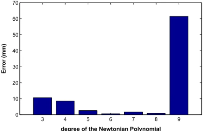
In Fig. 6, the maximum value of dr has been displayed in millimetres. For this comparison, the reference and approximated orbits of a CHAMP-like have been computed in the gravity field of the Earth over one day using EGM08 geopotential model with L=140 . As it was expected, by increasing the degree of Newton polynomial to approximate the ALFs, the accuracy of the approximated integration is increased at first. However, this trend continues only to a certain degree. The accuracy of the approximated orbit decreases after degree 7.

This result is in agreement with another experience of the polynomial approximation that using higher order polynomials could not always guarantee the accuracy improvement.

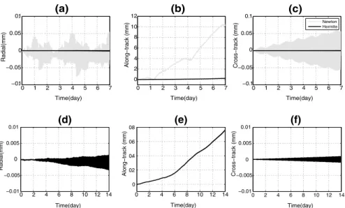
Based on the current finding, the results of the Hermitian interpolation is compared by the Newton polynomial of degree 6 as the most accurate Newtonian interpolator for the fast satellite orbit propagation. The approximation error of the proposed method leads to a difference between the reference and approximated orbits. The differences are presented in Fig. 7 for the Newtonian polynomial of degree 6 and Hermite polynomials over a week.

Figure 7 describes the difference between the reference and approximated orbits obtained by this methods over one week at radial, along-track, and cross-track direc- tions. As expected, the Hermitian method produces the better approximate orbit to the

(18) dr=‖𝐫^Ref.− 𝐫^Num.‖

Fig. 6 The error of the approxi- mated orbit obtained from the Newton polynomials of the different degrees (from 3 to 9) over 1 day

3 4 5 6 7 8 9

0 10 20 30 40 50 60 70

degree of the Newtonian Polynomial

Error (mm)

reference one. As the largest variation of a satellite in time lays in the along-track direc- tion, the largest error is expected to occur in the along-track component as well.

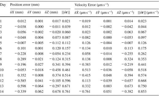
For illustrating more details, in Fig. 7d–f, the accuracy of the approximated orbit achieved by the Hermitian method is checked over two weeks too. Table 3 has been sum- marised the maximum error of the approximated orbit obtained from this method in term of the velocity and position vectors in the Earth-fix Inertial Cartesian system over two weeks. In addition, the norm of the position and velocity vectors are respectively added into the 4-th and 8-th columns of Table 3. Based on this results, the accuracy of the Her- mite approximated orbit is at sub-millimeter level in position, and in micrometer/s level in velocity for CHAMP. The high accuracy obtained from the proposed method in this section proves that it is an efficient approach for the fast satellite orbit propagation.

In addition to the results described above, it might be interesting to represent similar result for ODE113 in comparison with ODE45. Figure 8 illustrates the Euclidean norm of the 3D-differences between the reference and approximated orbits.

4.2 Geoid computation

As another important application, the ALFs is used for the computation of the gravity functional e.g. geoid. Given that the geopotential model EGM08 is developed up to degree/

order 2160 (Pavlis et al. 2012), the ability of the fast evaluated ALFs using the proposed idea for the gravity functional computation should be checked. Specially, we want to inves- tigate how much the computation error is due to the use of the approximated ALFs for geoid computation. For this propose, a new grid of the ALFs and their derivatives have been produced with latitude interval of 0.1 degree.

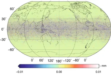
Then, two worldwide 3.6^�× 3.6^� high-resolution geoid models are computed fromthe EGM08 to degree/order 2160 one using the ordinary method of generation of ALFs and the other using the approximated ones, and their difference is shown in Fig. 9. The geoid

0 1 2 3 4 5 6 7

−

−0.05 0 0.05 1.

0

Radial(mm)

Time(day)

0 1 2 3 4 5 6 7

0 2 4 6 8 10 12

Along−track (mm)

Time(day)

0 1 2 3 4 5 6 7

−0.1

−0.05 0 0.05 0.1

Cross−track (mm)

Time(day)

Newton Hermite

(b) (c)

0 2 4 6 8 10 12 14

−0.01

−0.005 0 0.005

0.01 (d)

Radial(mm)

Time(day)

0 2 4 6 8 10 12 14

0 0.2 0.4 0.6

0.8 (e)

Along−track (mm)

Time(day)

0 2 4 6 8 10 12 14

−0.01

−0.005 0 0.005

0.01 (f)

Cross−track (mm)

Time(day)

(a)

1.

0

Fig. 7 The difference between the reference and approximated orbits, a, b, c obtained from the 6-degree Newton polynomial (light) and Hermite (dark) methods over one week; d, e, f obtained from the Hermite method over 2 weeks (numerical integrator is ode45)

undulation refers to the WGS84 ellipsoid. Although using the approximated ALFs leads to an error in the geoid computation with the maximum value of 1 mm, the approximation runs about 5 times faster than the ordinary method. As it was predicted, the geoid error is minimum near polar, because of the higher accuracy of the approximated ALFs in 𝜙=90^◦.

0 1 2 3 4 5 6 7

10⁻¹⁰ 10⁻⁸ 10⁻⁶ 10⁻⁴ 10⁻² 10⁰

Time (day)

Log of Error (mm)

Ode113 Ode45

Fig. 8 The difference between real and Hermite approximated orbits over a week using ode113 and ode45

Table 3 Maximum error of the approximated orbit obtained from the Hermite method Day Position error (mm) Velocity Error ( μm s⁻¹)

𝛿X (mm) 𝛿Y (mm) 𝛿Z (mm) ||𝛿𝐫|| 𝛿 ̇X ( μm s⁻¹) 𝛿 ̇Y ( μm s⁻¹) 𝛿 ̇Z ( μm s⁻¹) ||𝛿 ̇𝐫|| ( μm s⁻¹)

1 0.012 0.001 0.017 0.021 − 0.019 0.001 0.014 0.023

2 − 0.038 0.000 − 0.011 0.039 0.012 − 0.002 − 0.042 0.044

3 0.056 − 0.002 − 0.020 0.060 0.023 0.002 0.063 0.067

4 − 0.048 0.004 0.073 0.087 − 0.082 0.000 − 0.053 0.097

5 − 0.007 − 0.005 − 0.112 0.112 0.126 − 0.004 − 0.007 0.126

6 0.101 0.001 0.120 0.157 − 0.134 0.010 0.113 0.175

7 − 0.228 0.008 − 0.054 0.234 0.058 − 0.014 − 0.255 0.262

8 0.289 − 0.021 − 0.124 0.315 0.138 0.008 0.324 0.353

9 − 0.196 0.027 0.341 0.394 − 0.383 0.012 − 0.219 0.441

10 − 0.053 − 0.018 − 0.458 0.461 0.513 − 0.036 − 0.058 0.518

11 0.352 − 0.008 0.374 0.514 − 0.415 0.048 0.394 0.574

12 − 0.585 0.041 − 0.105 0.596 0.113 − 0.039 − 0.657 0.668

13 0.598 − 0.064 − 0.297 0.671 0.332 0.003 0.673 0.750

14 − 0.339 0.062 0.678 0.761 − 0.761 0.051 − 0.382 0.853

5 Conclusions

In this paper, the Newtonian and Hermitian approximations are suggested for the fast eval- uation of the ALFs instead of using the ordinary recursive formulae. The Hermite method delivers the values of ALFs with acceptable level of error, because of using of the first- and second-derivatives as well as the function values. In order to show the efficiency of the pro- posed method, the CPU-times needed for the ALFs evaluations using proposed and traditional methods were measured. Results show that the proposed method can evaluate the ALFs sig- nificantly faster, about 9 times for L=1290 with maximum error of 10⁻⁴ . This idea is effec- tive in accelerating the computation even for low degree, about L=20 , by speed-up factor 2 with maximum error of 10⁻¹⁴ . The effect of the error of the approximated ALFs has been tested in the satellite orbit propagation, and geoid computation. By approximating the ALFs as the most time-consuming part of the computations, the satellite orbit and geoid could be com- puted at least 2 and 5 times faster, respectively. The errors of the fast-propagated approximated orbit using the Hermite method in the position, and velocity vectors were below millimeter, 10μm s⁻¹ over two weeks for a CHAMP-like satellite orbit. In the case of the geoid compu- tation, the error due to the approximated ALFs is less than 1 mm. It is a sufficient and ideal accuracy for many applications in the space and geoscience.

0˚ 60˚ 120˚ 180˚ −120˚ −60˚ 0˚

−60˚

−30˚

0˚

30˚

60˚

−0.01 0.00 0.01

mm

Fig. 9 Error of the geoid computation due to the use of the approximated ALFs

Appendix A

The Earth’s gravity acceleration in the Earth-centered inertial frame is computed using (Keller and Sharifi 2005)

In this equation P̄^′_nm is the first order derivative of the associated Legendre function ( degree=n and order=m ) with respect to the latitude ( 𝜑 ). The first order derivative of the ALFs could be computed based on the ALFs themselves (Robin 1957), and C̄_nm and S̄_nm are the degree-n and order-m Stokes coefficients (e.g. Hofmann-Wellenhof and Moritz 2006).

where

Matlab code description

There are one main function needed for the ALFs computation and two related program files which have been used to create the required grid data. The main source functions and scripts are listed bellow.

1. 𝙰𝙿𝚗𝚖𝙷.𝚖 : This sub-routine is used for the fast computation of the ALFs using the Her- mite polynomial approximation based on Eq. (13).

2. 𝙿𝚗𝚖𝙶𝚛𝚒𝚍.𝚖 : This script is used for generating the needed grid-data.

3. 𝙿.𝚖 : This function is used to compute the ALFs and their first- and second-derivatives.

4. 𝚎𝚡𝚊𝚖𝚙𝚕𝚎.𝚖 : In this script, the fast computation of the ALFs has been described for more details.

In order to use this source codes, please follow the steps: (i) Run 𝙿𝚗𝚖𝙶𝚛𝚒𝚍.𝚖 to produce and save the grid file, the latitude interval of 0.5^◦ is suggested for the fast orbit propagation.

(ii) At the first of the computation, load the grid file. Once loaded, nothing more loading is needed. (iii) Run 𝙰𝙿𝚗𝚖𝙷.𝚖 for any desired latitude. As an example, run 𝚎𝚡𝚊𝚖𝚙𝚕𝚎.𝚖 after producing grid file.

(19) 𝐫_g=

⎡⎢

⎢⎢

⎣

cos(𝜑)cos(𝜆) ^{−sin(𝜑)cos(𝜆)}

r

−sin(𝜆) rcos(𝜑)

cos(𝜑)sin(𝜆) ^{−sin(𝜑)sin(𝜆)}

r

cos(𝜆) rcos(𝜑)

sin(𝜑) ^cos(𝜑)

r 0

⎤⎥

⎥⎥

⎦

×GM r

�∞ n=0

�R r

�ⁿ�ⁿ

m=0

⎡⎢

⎢⎢

⎣

−ⁿ⁺¹

r

�

C_nmcos(m𝜆) +S_nmsin(m𝜆)

�

P_nm(sin(𝜑))

�C̄_nmcos(m𝜆) + ̄S_nmsin(m𝜆)�P̄^�_nm(sin(𝜑))

�−mC̄_nmsin(m𝜆) +mS̄_nmcos(m𝜆)�P̄_nm(sin(𝜑))

⎤⎥

⎥⎥

⎦

(20) P̄^�_nm= 𝜕 ̄P_nm

𝜕𝜑 =K_nmP̄_n,m+1−mtan(𝜑) ̄P_nm

(21) K_nm=

√

(2− 𝛿_m,0)(n−m)(n+m+1) 2

Listing 1 The input and output of the functionAPnmH.m

Listing 2 The setup and result of the scriptPnmGrid.m

Listing 3 The input and output of the functionP.m

Listing 4 An example of the fast computed ALFs

References

Abramowitz M, Stegun IA (1972) Handbook of mathematical functions: with formulas, graphs, and math- ematical tables. Courier Dover Publications, New York 55

Atkinson KE (2008) An introduction to numerical analysis. Wiley, New York

Bettadpur SV, Schutz BE, Lundberg JB (1992) Spherical harmonic synthesis and least squares computations in satellite gravity gradiometry. Bull Géod 66(3):261–271

Boyd JP, Alfaro LF (2013) Hermite function interpolation on a finite uniform grid: defeating the runge phe- nomenon and replacing radial basis functions. Appl Math Lett 26(10):995–997

Cheong HB, Park JR, Kang HG (2012) Fourier-series representation and projection of spherical harmonic functions. J Geod 86(11):975–990

Dormand JR, Prince PJ (1980) A family of embedded Runge–Kutta formulae. J Comput Appl Math 6(1):19–26

Embree M (2010) Numerical analysis I. Lecture notes. Rice University, pp 1–207

Eshagh M (2009) Impact of vectorization on global synthesis and analysis in gradiometry. Acta Geod Geo- phys Hung 44(3):323–342

Eshagh M, Abdollahzadeh M (2010) Semi-vectorization: an efficient technique for synthesis and analysis of gravity gradiometry data. Earth Sci Inform 3(3):149–158

Eshagh M, Abdollahzadeh M (2012) Software for generating gravity gradients using a geopotential model based on an irregular semivectorization algorithm. Comput Geosci 39:152–160

Földváry L (2015) Sine series expansion of associated Legendre functions. Acta Geod Geophys 50(2):243–259

Fukushima T (2012) Numerical computation of spherical harmonics of arbitrary degree and order by extending exponent of floating point numbers: first-, second-, and third-order derivatives. J Geod 86(11):1019–1028

Gautschi W (1967) Computational aspects of three-term recurrence relations. SIAM Rev 9(1):24–82 Haken H, Wolf HC (2004) Molecular physics and elements of quantum chemistry: introduction to experi-

ments and theory. Springer, Berlin

Hildebrand FB (1987) Introduction to numerical analysis. Courier Corporation, North Chelmsford Hobson EW (1955) The theory of spherical and ellipsoidal harmonics. CUP Archive, Cambridge Hoffman JD, Frankel S (2001) Numerical methods for engineers and scientists. CRC Press, Boca Raton Hofmann-Wellenhof B, Moritz H (2006) Physical geodesy. Springer Science & Business Media, Berlin Holmes SA, Featherstone WE (2002) A unified approach to the Clenshaw summation and the recur-

sive computation of very high degree and order normalised associated Legendre functions. J Geod 76(5):279–299

Hwang C, Lin MJ (1998) Fast integration of low orbiter’s trajectory perturbed by the earth’s non-sphericity.

J Geod 72(10):578–585

Ilk KH (1983) Ein Beitrag zur Dynamik ausgedehnter Körper: Gravitationswechselwirkung. Deutsche Geo- daetische Kommission Bayer. Akad. Wiss., 288

Kaula WM (2000) Theory of satellite geodesy: applications of satellites to geodesy. Courier Dover Publica- tions, New York

Keller W, Sharifi M (2005) Satellite gradiometry using a satellite pair. J Geod 78(9):544–557 Kolb WM (1984) Curve fitting for programmable calculators. 3rd edn, Syntec inc, Bowie, MD

Lundberg JB, Schutz BE (1988) Recursion formulas of legendre functions for use with nonsingular geo- potential models. J Guid Control Dyn 11(1):31–38

Montenbruck O, Gill E (2000) Satellite orbits: models, methods, and applications, 1st edn. Springer, Berlin

Pavlis NK, Holmes SA, Kenyon SC, Factor JK (2012) The development and evaluation of the Earth Gravita- tional Model 2008 (EGM2008). J Geophys Res Solid Earth 117:1–38

Phillips GM (2003) Interpolation and approximation by polynomials, vol 14. Springer, Berlin Reigber C, Lühr H, Schwintzer P (2002) CHAMP mission status. Adv Space Res 30(2):129–134 Robin L (1957) Fonctions sphériques de Legendre et fonctions sphéroidales, t. 1. Gauthier-Villars, Paris Rothwell EJ, Cloud MJ (2001) Electromagnetics. CRC Press, Boca Raton

Seeber G (2003) Satellite geodesy: foundations, methods, and applications. Walter de Gruyter, Berlin Shampine LF, Reichelt MW (1997) The Matlab ode suite. SIAM J Sci Comput 18(1):1–22

Sharifi M, Seif M (2014) A new family of multistep numerical integration methods based on hermite inter- polation. Celest Mech Dyn Astron 118(1):29–48

Sharifi MA (2006) Satellite to satellite tracking in the space-wise approach. Ph.D. thesis, University of Stuttgart

Sneeuw N, Bun R (1996) Global spherical harmonic computation by two-dimensional fourier methods. J Geod 70(4):224–232

Szegö G (1975) Orthogonal polynomials, 4th edn. American Mathematical Society, Providence

Yang WY, Cao W, Chung TS, Morris J (2005) Applied numerical methods using MATLAB. Wiley, New York