Multifractal and entropy analysis of resting-state
electroencephalography reveals spatial organization in local
dynamic functional connectivity
frigyes Samuel Racz, orestis Stylianou , peter Mukli & Andras eke
Functional connectivity of the brain fluctuates even in resting-state condition. It has been reported recently that fluctuations of global functional network topology and those of individual connections between brain regions expressed multifractal scaling. To expand on these findings, in this study we investigated if multifractality was indeed an inherent property of dynamic functional connectivity (DFC) on the regional level as well. Furthermore, we explored if local DFC showed region-specific differences in its multifractal and entropy-related features. DFC analyses were performed on 62-channel, resting- state electroencephalography recordings of twelve young, healthy subjects. Surrogate data testing verified the true multifractal nature of regional DFC that could be attributed to the presumed nonlinear nature of the underlying processes. Moreover, we found a characteristic spatial distribution of local connectivity dynamics, in that frontal and occipital regions showed stronger long-range correlation and higher degree of multifractality, whereas the highest values of entropy were found over the central and temporal regions. The revealed topology reflected well the underlying resting-state network organization of the brain. The presented results and the proposed analysis framework could improve our understanding on how resting-state brain activity is spatio-temporally organized and may provide potential biomarkers for future clinical research.
Analyzing how different regions of the brain dynamically interact emerged as a new frontier of neuroscience in the past decades1,2. Such studies investigating brain functional connectivity (FC) made an immense contribution to the still expanding knowledge on how functional brain networks are organized in space and time2,3. Moreover, it has been widely recognized that FC carries great potential for future clinical applications as well4–6. Ever since the fluctuating nature of resting-state FC has been explicitly demonstrated7,8, a new trend developed within the connectivity field aiming on describing FC in a time-resolved manner9–11. This approach investigating dynamic functional connectivity (DFC) allows for a more detailed analysis of brain function either in resting-state condi- tion or during task-modulation12. Also, a dynamic approach to FC has been shown by several studies outperform- ing traditional stationary techniques when it comes to distinguish between healthy and pathological conditions such as schizophrenia13–16 or Alzheimer’s disease17.
Investigating DFC shed light on several important properties on how neural activity, and most importantly, interactions between neuronal populations are temporally organized. The nonlinear nature of functional cou- pling between brain regions has been confirmed by Stam et al.18 based on electroencephalography (EEG) and magnetoencephalography (MEG) recordings. In a functional magnetic resonance imaging (fMRI) study Lahaye and coworkers highlighted the importance of the nonlinear nature of interactions between blood oxygen level dependent (BOLD) signals when identifying significant connections19. Their work demonstrated that taking into account the non-linearity of interrelated dynamics makes a model more sensitive than when it is based only on methods of linear correlation. Jia and colleagues20 used Sample Entropy21,22 (SampEn) analysis for characterizing the temporal complexity of individual connections as well as average FC of each region of interest (ROI), thus
Semmelweis University, Department of Physiology, 37-47 Tuzolto street, 1094, Budapest, Hungary. Correspondence and requests for materials should be addressed to A.E. (email: eke.andras@med.semmelweis-univ.hu)
Received: 3 April 2019 Accepted: 24 August 2019 Published: xx xx xxxx
open
stressing the need and importance of revealing non-trivial features of DFC. They created a spatial SampEn map of the brain as well as identified an age-related decrease in the SampEn of connections that link the amygdala to various regions of the cortex; a pattern that was absent in patients with schizophrenia20.
DFC has also been shown having several scale-free properties, meaning that fluctuations in neuronal synchro- nization cannot be characterized by a single time scale. Instead, such processes express long-range correlations (LRC) resulting in a power-law distribution of their statistical properties23. Gong and coworkers investigated the dynamic phase synchronization in alpha band EEG between randomly selected brain regions and found that fluc- tuations in the length of synchronization events followed a scale-invariant pattern24. Stam and de Bruin showed that global EEG synchronization also expressed scale-free dynamics in all frequency bands with stronger LRC in eyes closed than eyes open state25. Van de Ville and colleagues investigated the dynamics of EEG microstates and revealed that transitions between different microstates also occurred according to scale-free dynamics26.
In a recent study utilizing functional near-infrared spectroscopy (fNIRS) imaging and a dynamic graph theoretical approach it has been confirmed that DFC of the prefrontal cortex exhibited not only scale-free but multifractal dynamics27, meaning that the scale-free property itself varied over time. In case of multifractality, dynamics has to be characterized with a set of scaling exponents instead of a single scale-free parameter, and the degree of multifractality is captured in the width of the distribution of such scaling exponents28,29. The mul- tifractal nature of global DFC was subsequently demonstrated in the whole cortex as well using EEG mapping30. Moreover, the scope of observations was extended beyond global FC to synchronization levels between pairs of brain regions, which demonstrated that individual functional connections themselves also fluctuated according to true multifractal dynamics30. Finally, a characteristic spatial distribution of the individual connections was found in terms of their multifractal properties, where connections linking regions of the frontal and prefrontal cortex expressed stronger LRC and degree of multifractality30. Similarly to previous studies28,31–33, it has also been verified that the observed multifractality was – at least partly – a consequence of the nonlinear nature of the investigated process.
From the results of Jia et al.20 and Racz et al.30, it is apparent that functional connectivity dynamics vary across different brain regions, which may also bear clinical significance. Interpositioned between global network topol- ogy and individual connections, local connectivity of each ROI captures a different aspect of organization; namely of how a given ROI is functionally integrated within the whole dynamic system of the brain. Therefore, the first objective of this study was to verify if multifractality was indeed an inherent property of local DFC. This would enhance our previous approaches where only multifractal properties of global network topology and individual connections were considered27,30. In order to realize this goal, we performed DFC analyses on resting-state EEG recordings via estimating dynamic synchronization levels between a set of cortical regions. Subsequently, a meas- ure of local connectivity was computed from the levels of synchronization in a time-resolved manner, yielding time series capturing local DFC for every investigated brain region. Finally, these acquired time series were made subject to multifractal analysis and statistical testing to verify their presumed multifractal nature. Our second aim was to investigate how the scale-free nature of local DFC varied across different ROIs i.e. to see if localiza- tion had a significant effect on the multifractal characteristics of local dynamic connectivity. At this end, we also investigated the localization-related differences of another widely used nonlinear measure of signal complexity, Permutation Entropy34 (PermEn) in order to offer a more comprehensive description of the spatio-temporal structuring of local DFC. We performed statistical tests to verify if localization had a significant effect on the temporal complexity of DFC, while also performed surrogate data testing to see if the spatial ordering could be destroyed by randomly shuffling electrode localizations. Combining these various methods, our goal was to obtain spatial maps that capture the complexity of local functional connectivity. Acquiring such spatial maps could not only help to enhance our understanding on how the brain as a complex system is spatio-temporally organized, but also provide potential biomarkers for future clinical investigations.
Results
Assessing the temporal complexity of local DFC. An openly available dataset containing resting-state, 62-channel EEG recordings of 12, young healthy participants35 was analyzed. After preprocessing the raw EEG data (see Materials and Methods), the dynamic i.e. time-dependent synchronization levels between all pairs of channels were estimated using the Synchronization Likelihood (SL) method36. This yielded a set of synchroni- zation matrices – one for every time point – describing the dynamically changing connection structure of the cortical functional network. In these, cells contained the actual values of SL between the corresponding ROIs, rep- resenting the estimated strength of functional co-operation. Using the synchronization matrices, for every time point we characterized the local functional connectivity of each ROI by its connectivity strength (also termed weighted node degree; for details see Materials and Methods). This analysis eventually produced connectivity strength time series for all ROIs, capturing fluctuations of local DFC. Multifractal properties of these fluctuations were then estimated with focus-based multifractal signal summation conversion37 (FMF-SSC). Long-range corre- lation was described with the monofractal Hurst exponent H(2), while the degree of multifractality was captured in the difference between the generalized Hurst exponents obtained at the minimal and maximal generalized moments, termed ΔH15. We characterized the temporal complexity of local DFC with the normalized version of PermEn34. The whole analysis procedure was carried out in the five frequency bands traditionally used in EEG analysis (delta: 0.5–4 Hz, theta: 4–8 Hz, alpha: 8–13 Hz, beta: 13–30 Hz and gamma: 30–45 Hz).
Verifying multifractality and nonlinearity in local DFC. When analyzing empirical signals, multifrac- tality can result from several reasons such as a broad power-law distribution of signal values29, the presence of different long-range correlations28, the nonlinear nature of the process28, the finite size of the time series38 or mere numerical noise37. Since only multifractality related to the presence of LRC and nonlinearity bears physi- ological significance, we performed surrogate data testing for each investigated time series to exclude the other
irrelevant cases of multifractality. In that, (i) we checked if the process was indeed scale-free as manifested in a 1/fβ spectra and (ii) by shuffling the time series we verified that the scale invariance was indeed a result of LRC.
Then (iii) by comparing the estimates of multifractality of the actual time series to those of strictly monofractal signals we excluded the possibility of numerical and multifractal background noise. Finally, (iv) we performed phase randomization in order to see if the observed multifractality was a consequence of nonlinear dynamics. The presence of nonlinearity was also investigated through PermEn, where (v) PermEn of the original time series was compared to those of phase randomized surrogates. Results obtained by this testing framework revealed that local DFC indeed expressed scale-free dynamics, that was found as a consequence of LRC in the signal. The observed multifractality could be clearly distinguished from multifractal background noise and diminished significantly when the nonlinear property of the time series was eliminated by phase randomization. However, PermEn failed to identify nonlinear behavior in the theta, alpha and beta bands. Detailed results for all test steps and frequency bands are shown in Table 1.
Spatial organization in the complexity of local DFC. We used Friedman tests to determine if localiza- tion had a significant effect on the assessed values of H(2), ΔH15 and PermEn. To further explore the existence of a significant topology, Friedman tests were repeated on n = 100 spatial surrogates, where for each subject the estimates of H(2), ΔH15 and PermEn were randomly assigned to the 62 channel locations. To check how similar the spatial distribution of each complexity metric was among individual subjects, we calculated Kendall’s coeffi- cient of concordance39 (W). We used Cohen’s interpretation guideline40, where W[0 1 0 3). . corresponds to small effect, while W[0 3 0 5). . and W ≥ 0.5 corresponds to moderate and strong effects, respectively. Non-parametric pairwise comparison of all measures in all frequency bands were performed using Kendall’s τ coefficient to see if their topology appeared similar.
In most cases, we found significant regional differences, except for H(2) in the delta, and for ΔH15 in the theta and alpha bands. Kendall’s W mostly indicated small concordance among subjects for H(2) and ΔH15, however the spatial pattern appeared strongly consistent for PermEn in alpha and higher frequency ranges (shown in detail in Table 2). Spatial surrogate testing further confirmed the existence of a significant topology, as Friedman tests were not significant (p > 0.05) in all cases when performed on spatially randomized data. Kendall’s τ revealed that all three parameters showed consistent spatial differences, except when comparing H(2) with ΔH15 in the delta band, as well as H(2) and PermEn with ΔH15 in the theta band. These exceptions however are hardly surprising as in these frequency bands the spatial distribution of at least one of the complexity parameters were random/
homogenous (see below). When investigating dynamic properties of local FC on the level of intrinsic networks, we found that the revealed channel-wise topology reflected well the functional organization of the brain, espe- cially in the higher frequency bands.
Spatial maps. To observe the spatial distributions of the three investigated dynamic measures, we created group-level spatial maps after standardizing (z-scoring) the values of H(2), ΔH15 and PermEn on the sub- ject level. Assuming x to be be the investigated measure, z was obtained as (x − μ)/σ; where μ and σ are the within-subject mean and standard deviation, respectively. H(2) of local DFC was found to express a consistent topology in the theta and higher frequency bands, where frontal-prefrontal and occipital regions could be char- acterized with higher H(2) values, while in the delta band it showed a homogenous distribution (Fig. 1, upper
Power-law
spectrum Long-range
correlations Multifractal
noise Nonlinearity
(ΔH15) Nonlinearity (PermEn)
Delta 96.9 ± 1.8% 100% 100% 100% 99.6 ± 1.0%
Theta 95.7 ± 2.1% 100% 100% 99.5 ± 1.1% 15.5 ± 6.9%
Alpha 95.6 ± 2.2% 100% 100% 98.7 ± 1.7% 18.4 ± 6.4%
Beta 94.6 ± 2.0% 100% 100% 88.0 ± 7.1% 25.8 ± 14.4%
Gamma 95.3 ± 2.5% 100% 100% 97.0 ± 1.9% 88.3 ± 6.3%
Table 1. The percentage of the local DFC time series averaged across subjects for all five tests, in all frequency bands (mean ± standard deviation). Chi-square test was used separately for each case (frequency band and test) to verify that channel location had no significant effect on the test outcome (p > 0.05 in all cases), i.e. the testing framework yielded similar results for all channels.
Delta Theta Alpha Beta Gamma
H(2) Friedman p 0.1105 <0.0001 <0.0001 <0.0001 <0.0001
Kendall’s W 0.1022 0.2748 0.2722 0.4263 0.3203
ΔH15 Friedman p 0.0058 0.1596 0.5878 <0.0001 <0.0001
Kendall’s W 0.1262 0.0983 0.0791 0.2164 0.2121
PermEn Friedman p 0.006 0.0001 <0.0001 <0.0001 <0.0001
Kendall’s W 0.126 0.1499 0.5066 0.6109 0.5886
Table 2. Results for the Friedman tests (p-values) and Kendall’s W values for all three investigated measures in all frequency bands. Values representing significant effect of localization are marked in bold.
panel). In the delta band, local connectivity dynamics could be characterized with higher ΔH15 over the central and temporal regions, however in the beta and gamma bands the opposite topology emerged, with higher values over the frontal-prefrontal and occipital regions (Fig. 1, middle panel). ΔH15 was found evenly distributed over the cortex in the theta and alpha bands. When exploring the spatial distribution of PermEn we found that in the delta band the frontal and occipital regions expressed higher temporal complexity. However, in the higher fre- quency bands again the opposite topology was found, where the central and temporal regions could be described with higher values of PermEn (Fig. 1, lower panel).
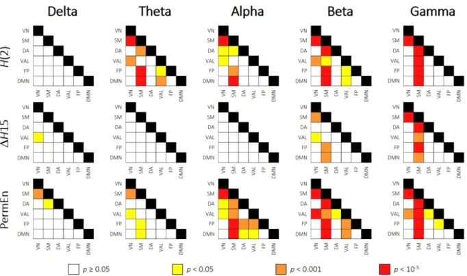
Resting-state networks. Also, to see if the revealed channel-wise topology resembled the intrinsic net- work organization of the brain, we sorted the 62 channels into 6 groups to represent the activity of previously established resting-state networks41 (RSNs). These included the visual (VN), somatomotor (SM), dorsal attention (DA), ventral attention and limbic (VAL), frontoparietal (FP) and default mode (DMN) networks. Based on the work of Giacometti and colleagues42, each EEG channel was assigned to an RSN whose activity the particular electrode most likely recorded (for details, see Materials and Methods and Fig. 7). Following this parcellation, we averaged the H(2), ΔH15 and PermEn values belonging to the same networks on the subject level. Subsequently, the 6 RSNs were compared with repeated-measures analysis of variance. We found that the previously revealed spatial differences reflected well the intrinsic RSN organization of the brain. Multifractal parameters and PermEn of the RSNs for all frequency bands are presented collectively in Fig. 2, while results of the pairwise comparisons are shown correspondingly in Fig. 3. From the results it is apparent that the visual, frontoparietal and default mode networks expressed mostly similar characteristics. In the higher frequency bands regions with the lowest H(2) and ΔH15, whilst highest PermEn values were mainly associated with the somatomotor network. Especially in the theta, alpha and gamma bands the combined ventral attention and limbic networks could also be charac- terized with lower H(2) and higher PermEn values than in the visual, frontoparietal and default mode networks.
Except for SM in the beta and gamma bands, VAL also expressed lower ΔH15 then the rest of RSNs. As expected from the channel-wise spatial maps, RSN dynamics in the delta band showed an opposite pattern when compared to higher frequency bands. Higher ΔH15 and lower PermEn values found in SM and VAL attest to this observa- tion. These differences were however less pronounced, as pairwise comparisons proved to be significant only for a limited number of cases (Fig. 3).
Discussion
In this study, we showed that fluctuations in local DFC expressed complex temporal structuring consistent with a true multifractal model of the observed dynamics. This – similarly to previous studies27–30 – was statistically verified by means of surrogate data testing. Further statistical testing revealed that this property indeed mani- fested independently of brain region, which inferred that multifractality of local DFC was a ubiquitous, genuine property in the whole cortex. Previous studies already demonstrated the scale-free nature of DFC by means of global connectivity25,26 as well as on the level of inter-regional connections24. The true multifractal nature of both Figure 1. Spatial maps of multifractal parameters and PermEn. Group-averaged spatial maps of H(2) (upper), ΔH15 (middle) and PermEn (lower) reveal characteristic topology in most of the cases. H(2) and PermEn appear to show the opposite pattern to each other, especially in the alpha and higher frequency bands. While the fronto-occipital patterns for the frequency ranges of theta and above are fairly consistent, those of the delta band is clearly seen as distinct. For visualization purposes, data was standardized (z-scored) on the subject-level in each case before group averaging to avoid the influence of inter-subject variability. Note, that standardization has no effect on rank-based statistics.
Figure 2. Resting-state network dynamics. Bar plots showing the H(2) (upper), ΔH15 (middle) and PermEn (lower) of the 6 RSNs in all five frequency bands. Vertical lines represent standard deviation from the mean. In most cases the somatomotor and ventral attention-limbic networks show clearly distinct characteristics from the rest of the RSNs. VN = visual network; SM = somatomotor; DA = dorsal attention; VAL = ventral attention and limbic; FP = frontoparietal; DM = default mode network.
Figure 3. Pairwise comparisons of resting-state networks. Pairwise comparisons of RSN dynamics are
presented as matrices, where rows and columns represent the RSNs, while cells contain the result of the pairwise comparison of corresponding RSNs. Different colors mark different levels of significance, while white cells indicate no significant difference as indicated by the legend. Dynamic characteristics of SM separated strongly from the rest of the RSNs in most frequency bands. VN = visual network; SM = somatomotor; DA = dorsal attention; VAL = ventral attention and limbic; FP = frontoparietal; DM = default mode network.
global network topology and that of individual connections were also confirmed recently27,30. Our present results contribute to this expanding body of knowledge by demonstrating that multifractality is an inherent property of DFC on the local level as well. Results of surrogate data testing performed on phase randomized surrogates impli- cate that the observed multifractality is related to the nonlinear nature of regional connectivity dynamics28,32. The presence of multifractal dynamics in physiological systems is often interpreted as resulting from stochastic feed- back regulation mechanisms43,44. This offers a plausible explanation indeed, considering the mostly bidirectional nature of functional connections and the presence of both excitatory and inhibitory synapses in the brain. It is likely that similar regulatory effects could – at least in part – shape the dynamics of regional functional connectiv- ity, however this notion clearly requires further research. Interestingly, the presence of nonlinearity could be more efficiently captured with multifractal time series analysis: phase randomization led to the vanishing of multifrac- tality, that was marked by a prominent decrease in ΔH15. On the contrary, PermEn remained almost unaltered following phase randomization instead of increasing, as expected. This suggests that multifractal analysis is a more sensitive technique in identifying nonlinear behavior than PermEn calculation. It should be noted however, that the general applicability of the former is limited as it is a model-based approach, whilst the latter is not34.
Although multifractality itself appeared as a universal property of local DFC independent of brain region, we found it manifesting to various extent at different ROIs. More precisely, values of H(2) and ΔH15 showed characteristic spatial organization in most frequency bands. In the higher range (beta and gamma in particular), the observed topology of H(2) and ΔH15 appeared quite similar, with higher values over the frontal and occipital regions. This pattern partly resembles the spatial distribution found in the same frequency bands in a previous work of Racz et al.30 when investigating the multifractal nature of individual connections, where connections with higher H(2) and ΔH15 values were localized mainly to the frontal and prefrontal cortex. Note however, that in that study the electrode density over the occipital and parietal cortices was sparse, likely preventing this pattern from manifesting fully. The same topology of H(2) still turned out to be significant (see Table 2) in the alpha and theta bands, however in the delta band its spatial distribution appeared random. On the contrary, the opposite topology of ΔH15 was found in the delta band, showing higher values over dorsal PFC and the temporal lobes. This peculiar behavior of the delta band – i.e. expressing inverse region-specific differences in multifractal characteristics when compared to higher frequency bands – has also been observed previously30. While this study understandably limits any further elaboration on the physiological underpinning of these findings, nev- ertheless it highlights the importance of the observed phenomenon. It appears worthwhile for future research to investigate delta band DFC under more suitable experimental conditions such as during sleep, where delta activity is more prominent. Values of PermEn also showed characteristic regional differences in the theta range and above, that resembled the exact opposite of the topology found in H(2) i.e. highest values over the central and temporal regions. In the delta band, a different distribution of PermEn was revealed with lower estimates over the somatomotor and temporal regions, however in that case the state space reconstruction was ill-conditioned: as the embedding dimension allowed for 25! possible permutations, a signal length of order 1026 would have been required for a reliable estimate of PermEn. Therefore, these results acquired in the delta band should only be treated as exploratory.
H(2) values in the gamma band were found in the close vicinity of 1, resembling a pure Brownian random walk (pink noise). In all other frequency bands H(2) fell within the range of 1.0 and 1.3 (Fig. 4), characterizing local DFC as an antipersistent process37 in consistence with the known nonstationarity of electrophysiological data23. This antipersistence implies that an increase in the local functional connectivity of a region is expected to be followed by a subsequent decrease. In other words, a state where the activity of a given ROI becomes more synchronized to those of the rest of the complex system – when the local connectivity of the ROI increases – will likely be followed by a state of functional decoupling.
Interpretation of the results regarding the differences found in ΔH15 is more challenging, as the relation of ΔH15 to neural activity is not fully established yet. Shimizu et al.45 reported an increase in the degree of multi- fractality in the occipital cortex during visual stimulation when investigating brain function through the BOLD signal. In a different fMRI study Ciuciu et al.46 utilized an auditory response paradigm and observed an increase in the degree of multifractality in the cerebellum, basal ganglia and fronto-parietal regions, while a decrease in the auditory and attentional systems. The cognitive relevance of multifractality was also investigated by Wink et al.47, finding that increased width of the multifractal spectrum (i.e. stronger multifractality) in the inferior frontal cortex was associated with faster response times in a face recognition task, but also with weaker accuracy. ΔH15 of local DFC reflects on the range in which scaling of local DFC varies over time, that also corresponds to the strength of nonlinearity in the process. From our results it appears that resting-state dynamic connectivity in the frontal and prefrontal regions (and also in the visual cortex) is regulated through more enhanced feedback mech- anisms, giving rise to increased variability in the scaling of local DFC. An opposite explanation seems reasonable regarding the somatomotor cortex, leastwise in resting-state condition. This behavior is hardly surprising though, as during rest the somatomotor system is presumably idle. Finally, the spatial pattern revealed for PermEn impli- cates a higher level of complexity in local DFC of the somatomotor system. From a different perspective, where white noise is considered as an infinitely complex process and therefore can be characterized with maximal entropy (in the normalized case, 1), local FC dynamics in the somatomotor system can be regarded closer to a random process when compared to the rest of the brain. This is well reflected in the values of PermEn usually falling between 0.8 and 0.9, meaning that local DFC is a highly complex process, although clearly distinguishable from white noise. It should be reiterated, that in most frequency bands the topology of PermEn highly resem- bled – although inversely – that of H(2). This level of resemblance raises questions about PermEn as a complexity estimator, which could be affected by the long-range correlations in the process. A recent work of Xiong and colleagues48 thoroughly investigated – beside other effects – the influence of LRCs on the performance of entropy estimators. According to their results, kernel-type estimators (such as PermEn) are biased by overestimating the absolute (theoretical) value of entropy, however this bias remains constant and very stable, independently of
the strength of LRC present in the signal48. Thus, even though PermEn would not necessarily yield the correct values of absolute entropy, the differences observed between various regions indeed indicate different levels of complexity, and not just merely reflect the different levels of long-range correlation. The relevance of this in this study is with PermEn appearing the most sensitive of the three parameters investigated, identifying the strongest channelwise spatial concordance with Kendall’s W > 0.5 in the alpha, beta and gamma bands.
By grouping the EEG channels to resemble intrinsic resting-state networks of the brain, we found that loca- tions with markedly different dynamical properties indeed corresponded well to intrinsic functional networks.
Most prominently, it was revealed that those regions with the lowest H(2), ΔH15 and highest PermEn values in most frequency bands corresponded mainly to the somatomotor network, the dorsal attention network and the combined ventral attention and limbic networks. Conversely, the highest H(2) values were consistently found in the visual, frontoparietal and default mode networks. Similar differences between scaling properties of resting-state networks were also observed in previous studies49,50. Specifically, He50 investigated the scale-free nature of the BOLD signal in numerous brain regions using detrended fluctuation analysis. Significant differences were identified between the monofractal Hurst exponent of various RSNs. In particular, the highest values were found in the default and visual networks, lowest values were produced by the motor network, the thalamus, the hippocampus and the cerebellum; while Hurst exponents of the attention and saliency networks were found in between50. Although our results were acquired using a different imaging modality, they are remarkably consistent with the results presented by He50, expanding on those by showing that not only monofractal, but multifractal and entropy-based measures, too, show significant differences among various RSN dynamics.
Several studies investigated the correspondence between RNSs reconstructed using fMRI and narrow-band electrophysiological activity in order to identify relationships between various RNSs and specific frequency bands. Some patterns were consistently verified by these studies, however there is also a considerable amount of inconsistency among the results. The visual network was found to show generally good correspondence to electrophysiological activity in all frequency bands except gamma51, with the correlation being the highest with the alpha and beta bands51,52. The somatomotor network was frequently reported to be strongly related to beta band activity51,53 and connections among the SM network could be best explained by beta band MEG activity52. Brain function within areas of the dorsal attention network was also most strongly related to alpha and beta band oscillations51,54. The electrophysiological correlates of the frontoparietal network were found mainly in the theta and gamma bands52,54. Finally, findings in the literature are the most inconsistent regarding the default mode network, which was reported to be associated with generally all frequency bands, albeit to a different extent51,53,54. Although to some degree most studies managed to associate RSNs to different frequency bands, a general conclu- sion was often drawn that RSNs most likely emerge from neural activity involving multiple frequencies. This was first demonstrated by Mantini et al.51, who showed that the dynamics of six investigated RSNs could be associated to various extent with electrophysiological oscillations of more than one frequency range. In fact, each RSN could be characterized by a specific set of electrophysiological correlates including all five frequency bands51. Similar conclusions were drawn by Hipp et al.53, who showed that even though there were cases where the activity of an RSN strongly represented neuronal activity in a specific frequency band (SM and beta), in general RSNs were Figure 4. Channel-wise box plots of H(2) in all frequency bands. H(2) values in the gamma band were found generally in the close vicinity of 1, representing a pure Brownian motion. In the lower frequency bands, H(2) mostly fell between 1 and 1.5, indicating an antipersistent process.
more likely to be associated with a mixture of concurrent activities at multiple frequencies. Note, that VN, SM and DA (among others such as the auditory network) are considered as parts of the extrinsic, while FP and DMN as constituents of the intrinsic higher order systems of the brain54,55 and thus they are often expected to show simi- lar inter-system and different between-system characteristics. In this present study, generally similar differences were found in the dynamics of local FC on the RSN level in all frequency bands. The SM and VAL networks were found most of the time to express different dynamic characteristics than the rest of RSNs (see Fig. 2), therefore our findings do not resemble the extrinsic-intrinsic organization of the brain. However in Fig. 3 it is apparent that each frequency band could be characterized with a unique set of differences, therefore our results are in support of those suggesting that RSNs are more likely to be associated with a mixture of neural activities emerging from a broad range of frequencies51,53.
Finally, we have to address certain limitations of this study. Although we were able to confirm the true multi- fractal nature of local resting-state DFC, the analyzed dataset consisted only of measurements with eyes closed.
In fact, global EEG dynamics56 and also scale-free properties of global DFC25,30 show several differences between eyes open and eyes closed states. Hence, in order to assess the influence of cortical desynchronization on multi- fractal properties of local DFC it would be indeed instructive to investigate state-related differences. Alterations in functional connectivity related to various task-response paradigms were already demonstrated using either static57–59 or dynamic12,60 approaches alike. As multifractal analysis proved to be capable of identifying cortical regions with increased stimulation45,46, its combination with DFC and entropy analysis could provide an even more sensitive tool in investigating the neuronal response to various external stimuli. Also, for the sake of simplic- ity in this study we characterized local functional connectivity only with one measure that is basically equivalent to the weighted node degree61. However, several other local properties of functional networks can be considered, such as the clustering coefficient62, local efficiency63 or centrality-related measures64. Inclusion of such measures in future studies could be beneficial. Probably the most severe drawback of the present study is the lack of exact source localization of the EEG signal, that would allow for a more precise brain parcellation and more direct estimation of neural activity of various RSNs65,66. In this regard, our procedure to parcellate the set of EEG elec- trodes in reference to intrinsic RNSs based on the probability maps provided by Giacometti et al.42 (see Materials and Methods) can be only regarded as a crude approximation, yet capable of producing results comparable to previous reports in the literature. The reason why we decided to follow this approach was that we would have liked to propose an analysis pipeline that was fully automatized and relied on EEG data only. For the same reason, all EEG preprocessing was carried out using automated algorithms. Likewise, starting parameters of the anal- ysis tools used during the analysis (i.e. SL, FMF-SSC and PermEn) were defined according to objective, purely data-driven criteria. The motivation behind these considerations was that this would allow such pipeline to be implemented with ease in a broad range of scenarios in possible future studies, including clinical conditions as well. Finally, it would be instructional to see how the results may depend on the electrode density of the measur- ing equipment. In order to address this issue, we repeated all steps of the analysis procedure using data only from the 19 electrodes localized at the international 10–20 positions. Detailed results of this approach are attached as Supplementary Material. We found that the characteristic topologies revealed based on all 62 channels could be very well reproduced using only 19 channels covering the whole cortex (see Fig. S1). Results regarding RSN dynamics (Figs S2 and S3) and concordance among subjects (Table S1) were also comparable, implicating that the patterns presented in this study were generally independent of electrode density.
conclusions
In this study, we demonstrated that DFC expressed multifractal dynamics when investigated on the local level and this property could be thoroughly verified through surrogate data testing. On this ground, we were able to characterize the temporal complexity of local DFC through its multifractal properties, utilizing also Permutation Entropy to have a more comprehensive description of system dynamics. We found that temporal characteris- tics of DFC varied significantly over the cortex, yielding characteristic spatial distributions of multifractal and entropy-related features. Moreover, the observed topologies reflected well the underlying functional organization of the brain. Our results shed light on previously unobserved features of spatio-temporal brain dynamics that are not only meaningful for a better understanding of physiological brain function, but could carry potential in future clinical applications as well.
Materials and Methods
Data and participants. In this study we analyzed a publicly available dataset of resting-state EEG recordings published and made freely available by Sockeel and colleagues35. The dataset consisted of the EEG recordings of twelve young, healthy participants (age 26.6 ± 2.1 years, 6 female, all right-handed). Measurements were carried out using a 62-channel BrainAmp system with a sampling rate of 5 kHz. The reference electrode was localized in the Cz position while a ground electrode was placed below the Oz position. During the measurements subjects were lying supine with their eyes closed while a recording equivalent to the sound produced by an MRI system was played to mimic the conditions of an MRI measurement. Similarly to Sockeel et al.35, only the last 300 seconds of the datasets (containing the resting-state recordings with eyes closed) were used in our study. Data was visually inspected and artifact-free segments with a length of 218 data points were selected for further analysis. The orig- inal study of Sockeel et al.35 was approved by the local ethics committee (Comité de Protection des Personnes–
Ile-de-France under the number CPP DGS2007-0555), measurements were carried out in accordance with the Declaration of Helsinki and all participants provided written informed consent.
Preprocessing. Preprocessing of raw EEG data was performed in Matlab (The Mathworks, Natick, MA, USA) using the Batch Electroencephalography Automated Preprocessing Platform67 (BEAPP). BEAPP operates using custom functions and scripts along with methods of the EEGLAB software package68. Data preprocessing
consisted of the following steps of the BEAPP pipeline: (i) Raw data was first band-pass filtered with lower and upper cutoff frequencies 0.5 Hz and 250 Hz, respectively, with additional ‘cleanline’ filtering to remove line noise at 50 Hz. (ii) Band-pass filtered data was then downsampled from 5 kHz to 500 Hz. Subsequently, (iii) artifact removal was carried out automatically using the Harvard Automated Processing Pipeline for Electroencephalography69 (HAPPE). HAPPE includes multiple steps of denoising such as a wavelet-enhanced independent component analysis (W-ICA) approach69 followed by independent component analysis (ICA) with automated component rejection using the Multiple Artifact Rejection Algorithm70,71 (MARA). Finally, (iv) data was again band-pass filtered to the frequency bands traditionally used in EEG analysis (delta: 0.5–4 Hz, theta:
4–8 Hz, alpha: 8–13 Hz, beta: 13–30 Hz and gamma: 30–45 Hz) using a 5th order Butterworth filter.
Dynamic functional connectivity estimation. Functional connectivity between all possible pairs of brain regions was estimated using the Synchronization Likelihood (SL) method36. SL utilizes a temporal embedding-based state-space reconstruction approach72 of dynamic processes x(t) = x1, x2, … xT and y(t) = y1, y2, … yT and estimates the probability of their generalized synchronization73. First, x(t) and similarly, y(t) are reconstructed in an m dimensional state space as a set of state space vectors using temporal embedding72 with time lag L as
= − … − − = − … − − .
X t( ) [ ,x xt t L, xt m( 1)L], ( )Y t [ ,y yt t L, yt m( 1)L] (1) Then, for each time point t, the k nearest neighbors of X(t) and Y(t) within a local neighborhood are identi- fied by their Euclidean distance. Finally, SL for every time point t is calculated as the conditional probability that the nearest neighbors of X(t) can be found at the same time points as the nearest neighbors of Y(t). Parameters of the SL algorithm (mainly m and L) were set in each case to fit the frequency bands and data sampling rate according to Montez et al.74 and are shown in Table 3. State space vectors can be close to each other not only due to recurrence but simply because they are close in time75. Therefore, to diminish this effect of temporal autocor- relation the direct neighborhood – as defined by the parameter w1 – of the actual state space vector X(t) is always excluded from the nearest neighbor search. Finally, the parameter w2 (w2 ≫ w1) defines the fixed neighborhood of X(t) where the nearest neighbor search is performed. For a detailed description and evaluation of the method the reader is referred to the original paper of Stam and van Dijk36. With SL being a probability-type measure it takes on values between 0 and 1 representing independence and complete synchronization, respectively. SL has several properties that make it an appealing choice for EEG-based DFC analysis as it is able to identify nonlinear dependencies between processes, robust against non-stationarities and it works in a time-resolved manner25,36. We set the internal thresholding parameter (that basically defines the number of nearest neighbors searched) to 0.05 as in previous studies25,30,76.
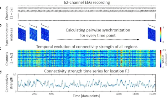
After calculating the pairwise SL time series from the 62-channel preprocessed EEG data (Fig. 5a), the acquired results could be organized into a set of synchronization matrices. More precisely, each matrix described the functional connection structure of the cortex at time point t (Fig. 5b). Based on these, local functional con- nectivity of each region was characterized with the connectivity strength (S) for every time point (Fig. 5c). S of channel i was calculated according to
∑
= − = ≠ S t( ) N1 SL t
1 ( )
i (2)
j j i N 1, ij
where SLij(t) is the value of SL between channels i and j at time point t and N is the number of channels. In a network theoretical approach the connectivity strength of a node is equivalent to its normalized weighted node degree61 and thus it captures the connectedness of the given ROI to the rest of the functional network. Finally, this procedure resulted in a connectivity strength time series for every channel (Fig. 5d), that captured the dynamics of local functional connectivity of the according brain region.
Multifractal time series analysis. The first 214 data points of the connectivity strength time series were sub- jected to FMF-SSC analysis37 to estimate their multifractal characteristics. The general (monofractal) signal sum- mation method77 (SSC) consists of the following steps: (i) the data is divided into segments (windows) of size s, (ii) for each segment the local linear trend is removed to avoid effects of non-stationarity, then (iii) the standard deviation σ of the detrended data is calculated in every window and finally (iv) averaged along the windows.
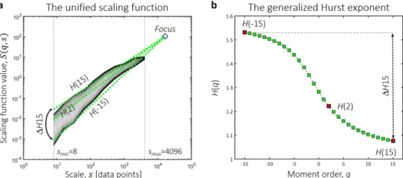
Subsequently v) the procedure described in steps (i–iv) is carried out for different scales (windows of different size) ranging from smin to smax. This yields a scaling function S(s) that is in general the averaged σ calculated as a function of window size. In case of scale-free signals, a power-law function can be fitted to S(s). The scaling exponent obtained this way is the monofractal Hurst exponent H, capturing the long-range correlation property of the process23. In the multifractal extension of SSC, the procedure described in steps (i–v) is repeated using a set of generalized moments (of order q) to magnify the effect of small (negative q values) and large (positive q values) fluctuations. This sequence of calculation yields the unified scaling function37 S(q, s) (Fig. 6a) according to
∑
σ υ=
υ=
S q s
N s
( , ) 1 ( , )
(3)
s
N q q
1
1 s
where Ns is the number of windows at scale s and υ is the index of the actual window of size s. Apart from calcu- lating standard deviation instead of fluctuation as the appropriate statistical measure, signal summation conver- sion is basically equivalent to the more widely used detrended fluctuation analysis78,79. Note, that in case of finite
empirical time series, replacing s in (3) with the total signal length basically eliminates the sum from the formula, thus making it independent from q. This results in the convergence of the values of S(q, s) calculated at different qs into a single point termed the focus37. Therefore, the focus can be used as a reference point during linear regres- sion, in that power-law functions are fitted to S(q, s) at each q (Fig. 6a). This procedure yields the generalized Hurst exponent, H(q) (Fig. 6b) that is defined as the scaling exponent of the fitted power-law function at gener- alized moment q. When the scaling function is plotted using double logarithmic scaling as in Fig. 6a, the fitted power-law functions appear as linear and estimates of H(q) are obtained as the slope of the function fitted to S(q, s) at moment q. Apart from making multifractal analysis robust in case of finite empirical signals, the focus-based regression also helps in enforcing the monotonously decreasing property of H(q)37, i.e. H(q1) ≥ H(q2) if q1< q2. The step-by-step process of FMF-SSC analysis is also illustrated in the Supplementary Video.
Parameters of the FMF-SSC analysis were set according to Mukli et al.37, with smin= 23, smax= 212 and
− − … + +
q { 15, 14, , 14, 15}. Multifractal properties were captured in two end-point parameters (Fig. 6b): H(2) which is equivalent to the monofractal Hurst exponent reflecting on the global long-range correlations in the signal23, and ΔH15 that is the difference between H(−15) and H(15), capturing the degree of multifractality in the process37. It is important to point out that these two measures adequately represent the multifractal nature of a process equivalently to the widely used singularity (also often termed multifractal) spectrum, as the latter can be obtained from the generalized Hurst exponent via Legendre transformation29,37. Consequently, H(2) is analo- gous – although not strictly equivalent – to the centre of the singularity spectrum, while ΔH15 captures the same property as the width of the singularity spectrum37.
Permutation entropy. As a first step of PermEn calculation, the investigated time series x(t) = x1, x2, … xT
is converted into a set of m-dimensional vectors X(t) using temporal embedding72 with time lag L. Then, values in each vector are replaced by their ranks within the actual vector. This step basically converts each vector into one of m! possible permutations of order m. The relative frequency of each permutation of type π in the process can be then calculated as
Figure 5. The process of dynamic functional connectivity estimation. Pairwise Synchronization Likelihood estimation is performed on the 62-channel EEG data (a) in a time-resolved manner. This yields a
synchronization matrix for every time point (b). From these matrices, connectivity strength of each region can be calculated in each instance (c), yielding connectivity strength time series. As a demonstration, the connectivity strength time series of region F3 is shown (d) from a representative subject, calculated from alpha band activity.
m L w1 w2
Delta 25 41 1968 2967
Theta 7 20 240 1239
Alpha 6 12 120 1119
Beta 8 5 70 1069
Gamma 6 3 30 1029
Table 3. Starting parameters of Synchronization Likelihood for all frequency bands. A method on how to objectively define m, L, w1 and w2 on data with explicit frequency limits is presented in Montez et al.74. The same values of m and L were used for Permutation Entropy calculation in each frequency band.
π = π
− − +
p of type permutation
T m L
( ) #
( 1) 1 (4)
giving the best estimate on the frequency of π in a finite time series34. Finally, Bandt and Pompe34 defined permu- tation entropy of order m as
∑
π πE m( )= − p( )log ( )p (5)
with the sum running over all m! possible π permutations of order m. Also, the upper limit of E(m) always appear to be equal to log !, therefore its normalized form can be acquired by dividing it by this upper limit. Thus m 0 ≤ E(m) ≤ 1 typically corresponds to different levels of complexity, with 0 standing for a completely predictable i.e. minimally complex, while 1 a maximally unpredictable i.e. random process34. Although there is no theoretical limit regarding the order m, by practical and computational considerations m is usually chosen in the range m{3 7}… , however with sufficient time series length higher values can be applied as well34. Also, in many appli- cations L = 1 is chosen, however in signals with explicit frequency limits it is advised to choose m and L so that the fluctuations present in the signal are well represented by the embedding80,81. Therefore, to remain consistent within our analyses, for all frequency bands we chose the same values of m and L as when calculating SL, as listed in Table 3.
Surrogate data testing. For the testing of power-law spectra, surrogate time series with equal length and spectral slope were generated using the spectral synthesis method82. The spectral slope β of the DFC time series was estimated by fitting a power-law function on their power spectrum using linear regression. Goodness of fit of the power-law function was assessed by the Kolmogorov distance D according to Clauset et al.83. If D of the original time series was within the mean ± 2σ range of those acquired from surrogate data, the time series was considered having a power-law spectrum50,83. For each time series 40 surrogate signals were generated, as this number corresponds to a 95% and 97.5% confidence level for two-sided and one-sided tests, respectively84,85.
Surrogates for LRC testing were created by shuffling the original time series, as shuffling destroys all long-range correlations and reduces the process into pure white noise, while having no effect on the distribu- tion of the values28,29. As H(2) of the original DFC time series were found always above 0.8, if it was outside the mean + 2σ range of those acquired from the surrogate time series the presence of LRC was verified. Again, 40 surrogates were generated for each time series.
Monofractal time series (n = 40) with equal length and H(2) were generated using the method of Davies and Harte86. ΔH15 values were acquired with FMF-SSC, and if ΔH15 of the DFC time series was larger than the mean + 2σ acquired from the monofractal signals, the case of multifractal background noise could be excluded.
Surrogates for the testing of nonlinearity (n = 40) were generated by Fourier transforming the original signal, randomizing its phases and then performing inverse Fourier transformation84. If the ΔH15 of the DFC time series was larger than the mean + 2σ acquired from the surrogates, the observed multifractality was considered as a consequence of nonlinearity. PermEn of the surrogates were also calculated and compared to those of DFC time series. If PermEn of the original time series was outside the mean ± 2σ range acquired from surrogates, the presence of nonlinearity was verified.
Figure 6. End-point parameters of multifractal time series analysis. The scaling function (a) is acquired by multifractal signal summation conversion. In that, standard deviation is calculated as a function of scale and the process is repeated along several statistical moments. The generalized (q-dependent) Hurst exponent (b) is acquired via linear regression with the focus used as a reference point. Global scale-invariance is described by H(2), while the degree of multifractality is captured as the difference between H(q) calculated at the minimal (−15) and maximal (15) moments.
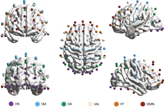
Brain parcellations. Brain parcellation was carried out manually according to the probability maps reported by Giacometti and colleagues42. These maps contain probabilities for EEG electrodes positioned in the 10–20, 10–10 and 10–5 configurations on which anatomical or functional network they most likely monitor42. We applied a non-overlapping parcellation scheme presented in Giacometti et al.42 where EEG electrodes were grouped to represent the activity of 7 intrinsic functional networks as identified by Yeo et al.41. Since some EEG electrodes were found to register the simultaneous activity of more than one intrinsic network42, in such cases the electrode was always assigned to the intrinsic network with the highest probability to achieve a non-overlapping parcellation. Also, as the electrode positions monitoring the ventral attention and limbic networks were strongly overlapping, we decided to treat these two networks jointly, resulting in a final number of 6 networks and their corresponding groups of channels (Fig. 7). Finally, the H(2), ΔH15 and PermEn values were averaged within each network on the subject level.
Statistical analysis. As requirements of a repeated measures analysis of variance were not fulfilled – because of the non-normal distribution of values in at least one of the channels (Kolmogorov-Smirnov test, p < 0.05) – we performed Friedman tests with a significance level of αs = 0.05 to investigate the effect of channel localization on the values of H(2), ΔH15 and PermEn. To further verify the existence of a significant topological distribution, Friedman tests were also performed on n = 100 spatial surrogates, where for each subject the estimated values of H(2), ΔH15 and PermEn were assigned to the 62 channel locations randomly. The accordance in the ranking of different electrode positions among subjects was estimated using Kendall’s coefficient of concordance39. Kendall’s W captures the similarity in the rank order of values and thus it reflects how similar the topological distribution appeared among the subjects. Non-parametric assessment of pair-wise correlation between the ranks of different complexity parameters was carried out using Kendall’s τ coefficient to determine whether the same subjects were responsible for the observed within-subject significant differences. When evaluating the difference between the dynamical measures of the 6 intrinsic brain networks, repeated measures analysis of variance could be applied as the datasets were normally distributed (Kolmogorov-Smirnov test, p > 0.05 in all cases) and the assumption of sphericity was not violated (Mauchley’s test, p > 0.05). Pairwise multiple comparisons between the networks were carried out separately for values of H(2), ΔH15 and PermEn using Bonferroni post-hoc tests with a significance level of αs = 0.05. Statistical analyses were performed using StatSoft Statistica 13.2.
Data Availability
The EEG data analyzed in this study was made publicly available without restrictions by Sockeel, et al.35 at http://
megfront.meg.chups.jussieu.fr/MEEG_data/data.tgz and http://datadryad.org/review?doi=doi:10.5061/dryad.
v9f16.
Figure 7. Electrodes were grouped to represent six resting-state networks: the visual network (VN, 10 channels), the somatomotor network (SM, 10 channels), the dorsal attention network (DA, 9 channels), the combined ventral attention and limbic networks (VAL, 12 channels), the frontoparietal network (FP, 8 channels) and the default mode network (DMN, 13 channels). Brain maps were created using the BrainNet Viewer software87 after electrode positions were transformed to match a template head using SPM 12b88. VN = visual network; SM = somatomotor; DA = dorsal attention; VAL = ventral attention and limbic; FP = frontoparietal;
DM = default mode network.
References
1. van den Heuvel, M. P. & Hulshoff Pol, H. E. Exploring the brain network: a review on resting-state fMRI functional connectivity. Eur Neuropsychopharmacol 20, 519–534, https://doi.org/10.1016/j.euroneuro.2010.03.008 (2010).
2. Friston, K. J. Functional and effective connectivity: a review. Brain Connectivity 1, 13–36, https://doi.org/10.1089/brain.2011.0008 (2011).
3. Bullmore, E. & Sporns, O. Complex brain networks: graph theoretical analysis of structural and functional systems. Nature reviews.
Neuroscience 10, 186–198, https://doi.org/10.1038/nrn2575 (2009).
4. Fox, M. D. & Greicius, M. Clinical applications of resting state functional connectivity. Front Syst Neurosci 4, 19, https://doi.
org/10.3389/fnsys.2010.00019 (2010).
5. Lee, M. H., Smyser, C. D. & Shimony, J. S. Resting-state fMRI: a review of methods and clinical applications. AJNR Am J Neuroradiol 34, 1866–1872, https://doi.org/10.3174/ajnr.A3263 (2013).
6. Stam, C. J. Modern network science of neurological disorders. Nature reviews. Neuroscience 15, 683–695, https://doi.org/10.1038/
nrn3801 (2014).
7. Chang, C. & Glover, G. H. Time-frequency dynamics of resting-state brain connectivity measured with fMRI. NeuroImage 50, 81–98, https://doi.org/10.1016/j.neuroimage.2009.12.011 (2010).
8. Zalesky, A., Fornito, A., Cocchi, L., Gollo, L. L. & Breakspear, M. Time-resolved resting-state brain networks. Proceedings of the National Academy of Sciences of the United States of America 111, 10341–10346, https://doi.org/10.1073/pnas.1400181111 (2014).
9. Hutchison, R. M. et al. Dynamic functional connectivity: promise, issues, and interpretations. NeuroImage 80, 360–378, https://doi.
org/10.1016/j.neuroimage.2013.05.079 (2013).
10. Preti, M. G., Bolton, T. A. & Van De Ville, D. The dynamic functional connectome: State-of-the-art and perspectives. NeuroImage 160, 41–54, https://doi.org/10.1016/j.neuroimage.2016.12.061 (2017).
11. Calhoun, V. D., Miller, R., Pearlson, G. & Adali, T. The Chronnectome: Time-Varying Connectivity Networks as the Next Frontier in fMRI Data Discovery. Neuron 84, 262–274, https://doi.org/10.1016/j.neuron.2014.10.015 (2014).
12. Sakoglu, U. et al. A method for evaluating dynamic functional network connectivity and task-modulation: application to schizophrenia. Magn Reson Mater Phy 23, 351–366, https://doi.org/10.1007/s10334-010-0197-8 (2010).
13. Damaraju, E. et al. Dynamic functional connectivity analysis reveals transient states of dysconnectivity in schizophrenia.
Neuroimage: Clinical 5, 298–308, https://doi.org/10.1016/j.nicl.2014.07.003 (2014).
14. Du, Y. H. et al. Interaction among subsystems within default mode network diminished in schizophrenia patients: A dynamic connectivity approach. Schizophrenia research 170, 55–65, https://doi.org/10.1016/j.schres.2015.11.021 (2016).
15. Yu, Q. B. et al. Assessing dynamic brain graphs of time-varying connectivity in fMRI data: Application to healthy controls and patients with schizophrenia. NeuroImage 107, 345–355, https://doi.org/10.1016/j.neuroimage.2014.12.020 (2015).
16. Rashid, B., Damaraju, E., Pearlson, G. D. & Calhoun, V. D. Dynamic connectivity states estimated from resting fMRI Identify differences among Schizophrenia, bipolar disorder, and healthy control subjects. Frontiers in human neuroscience 8, https://doi.
org/10.3389/fnhum.2014.00897 (2014).
17. Jones, D. T. et al. Non-Stationarity in the “Resting Brain’s” Modular Architecture. PloS one 7, https://doi.org/10.1371/journal.
pone.0039731 (2012).
18. Stam, C. J., Breakspear, M., van Cappellen van Walsum, A. M. & van Dijk, B. W. Nonlinear synchronization in EEG and whole-head MEG recordings of healthy subjects. Human Brain Mapping 19, 63–78, https://doi.org/10.1002/hbm.10106 (2003).
19. Lahaye, P. J., Poline, J. B., Flandin, G., Dodel, S. & Garnero, L. Functional connectivity: studying nonlinear, delayed interactions between BOLD signals. NeuroImage 20, 962–974, https://doi.org/10.1016/S1053-8119(03)00340-9 (2003).
20. Jia, Y. B., Gu, H. G. & Luo, Q. Sample entropy reveals an age-related reduction in the complexity of dynamic brain. Sci Rep-Uk 7, https://doi.org/10.1038/s41598-017-08565-y (2017).
21. Richman, J. S. & Moorman, J. R. Physiological time-series analysis using approximate entropy and sample entropy. Am J Physiol- Heart C 278, H2039–H2049 (2000).
22. Wang, Z., Li, Y., Childress, A. R. & Detre, J. A. Brain Entropy Mapping Using fMRI. PloS one 9, https://doi.org/10.1371/journal.
pone.0089948 (2014).
23. Eke, A., Herman, P., Kocsis, L. & Kozak, L. R. Fractal characterization of complexity in temporal physiological signals. Physiological measurement 23, 1–38 (2002).
24. Gong, P., Nikolaev, A. R. & van Leeuwen, C. Scale-invariant fluctuations of the dynamical synchronization in human brain electrical activity. Neuroscience letters 336, 33–36, https://doi.org/10.1016/S0304-3940(02)01247-8 (2003).
25. Stam, C. J. & de Bruin, E. A. Scale-free dynamics of global functional connectivity in the human brain. Human Brain Mapping 22, 97–109, https://doi.org/10.1002/hbm.20016 (2004).
26. Van de Ville, D., Britz, J. & Michel, C. M. EEG microstate sequences in healthy humans at rest reveal scale-free dynamics. Proceedings of the National Academy of Sciences of the United States of America 107, 18179–18184, https://doi.org/10.1073/pnas.1007841107 (2010).
27. Racz, F. S., Mukli, P., Nagy, Z. & Eke, A. Multifractal dynamics of resting-state functional connectivity in the prefrontal cortex.
Physiological measurement 39, 024003 (2018).
28. Ivanov, P. C. et al. Multifractality in human heartbeat dynamics. Nature 399, 461–465, https://doi.org/10.1038/20924 (1999).
29. Kantelhardt, J. W. et al. Multifractal detrended fluctuation analysis of nonstationary time series. Physica A 316, 87–114, https://doi.
org/10.1016/S0378-4371(02)01383-3 (2002).
30. Racz, F. S., Stylianou, O., Mukli, P. & Eke, A. Multifractal dynamic functional connectivity in the resting-state brain. Frontiers in Physiology 9, 1704 (2018).
31. Ashkenazy, Y. et al. Magnitude and sign scaling in power-law correlated time series. Physica A 323, 19–41, https://doi.org/10.1016/
S0378-4371(03)00008-6 (2003).
32. Gomez-Extremera, M., Carpena, P., Ivanov, P. & Bernaola-Galvan, P. A. Magnitude and sign of long-range correlated time series:
Decomposition and surrogate signal generation. Phys Rev E 93, 042201, https://doi.org/10.1103/PhysRevE.93.042201 (2016).
33. Bernaola-Galvan, P. A., Gomez-Extremera, M., Romance, A. R. & Carpena, P. Correlations in magnitude series to assess nonlinearities: Application to multifractal models and heartbeat fluctuations. Phys Rev E 96, 032218, https://doi.org/10.1103/
PhysRevE.96.032218 (2017).
34. Bandt, C. & Pompe, B. Permutation entropy: A natural complexity measure for time series. Physical Review Letters 88, https://doi.
org/10.1103/PhysRevLett.88.174102 (2002).
35. Sockeel, S., Schwartz, D., Pelegrini-Issac, M. & Benali, H. Large-Scale Functional Networks Identified from Resting-State EEG Using Spatial ICA. PloS one 11, https://doi.org/10.1371/journal.pone.0146845 (2016).
36. Stam, C. J. & van Dijk, B. W. Synchronization likelihood: an unbiased measure of generalized synchronization in multivariate data sets. Physica D 163, 236–251, https://doi.org/10.1016/S0167-2789(01)00386-4 (2002).
37. Mukli, P., Nagy, Z. & Eke, A. Multifractal formalism by enforcing the universal behavior of scaling functions. Physica A 417, 150–167, https://doi.org/10.1016/j.physa.2014.09.002 (2015).
38. Grech, D. & Pamula, G. Multifractal Background Noise of Monofractal Signals. Acta Phys Pol A 121, B34–B39 (2012).
39. Legendre, P. Species associations: The Kendall coefficient of concordance revisited. J Agr Biol Envir St 10, 226–245, https://doi.
org/10.1198/108571105x46642 (2005).