Analysis and Classification of Liquid Samples Using Spatial Heterodyne Raman Spectroscopy
Ardian B. Gojani1, Dávid J. Palásti,2,3 Andrea Paul,1 Gábor Galbács,2,3 and Igor B. Gornushkin1
1 Federal Institute for Material Research and Testing (BAM), Richard-Willstätter-Str. 11, 12489, Berlin, Germany
2 Department of Inorganic and Analytical Chemistry, University of Szeged, 6720 Szeged, Dóm Square 7, Hungary
3 Department of Materials Science, Interdisciplinary Excellence Centre, University of Szeged, 6720 Szeged, Dugonics Square 13, Hungary
Corresponding author email: igor.gornushkin@bam.de
Abstract
Spatial heterodyne spectroscopy (SHS) is used for quantitative analysis and classification of liquid samples. SHS is a version of a Michelson interferometer with no moving parts and with diffraction gratings in place of mirrors. The instrument converts frequency-resolved information into spatially resolved one and records it in the form of interferograms. The back-extraction of spectral information is done by the fast Fourier transform. A SHS instrument is constructed with the resolving power 5000 and spectral range 522–593 nm. Two original technical solutions are used as compared to previous SHS instruments: the use of a high-frequency diode-pumped solid- state (DPSS) laser for excitation of Raman spectra and a microscope-based collection system.
Raman spectra are excited at 532 nm at the repetition rate 80 kHz. Raman shifts between 330 cm–1 and 1600 cm–1 are measured. A new application of SHS is demonstrated: for the first time it is used for quantitative Raman analysis to determine concentrations of cyclohexane in
isopropanol and glycerol in water. Two calibration strategies are employed: univariate based on the construction of a calibration plot and multivariate based on partial least squares regression (PLSR). The detection limits for both cyclohexane in isopropanol and glycerol in water are at a 0.5 mass% level. In addition to the Raman–SHS chemical analysis, classification of six industrial oils (biodiesel, poly(1-decene), gasoline, heavy oil IFO380, polybutenes, and lubricant) is
performed using oils’ Raman–fluorescence spectra and principal component analysis (PCA). The oils are easily discriminated showing distinct non-overlapping patterns in the principal
component space.
Keywords: Spatial heterodyne spectroscopy, Raman spectroscopy, diode-pumped solid-state, DPSS, chemical analysis
Introduction
Spatial heterodyne spectroscopy (SHS) is a spectrometric method that combines dispersion- and interference-based techniques for obtaining spectroscopic information. It is a version of a
Michelson interferometer with no moving parts and with diffraction gratings in place of mirrors;
the operation principle is given in the Appendix. Briefly, the radiation from a light source is collimated and split between two arms of the interferometer which are terminated by diffraction gratings. The light dispersed by the gratings recombines at the beam splitter and produces Fizeau fringes that are imaged onto a charge-coupled device (CCD) or intensified CCD (ICCD)
detector. The frequency (wavelength)-resolved information is thus converted into the spatially resolved one and is recorded in the form of the interferogram, a system of parallel lines with alternating intensity and spatial periodicity. The spatial periodicity of the fringes depends on the wavelength of the dispersed light. The recovery of original spectra from interferograms is done using fast Fourier transform (FFT). Similar to other FT-based spectrometers, the SHS benefits from the simultaneous advantage of high throughput and high spectral resolution. SHS is also more robust and less sensitive to light source fluctuations owing to the use of fixed (non- scanning) gratings.1
The working principle of SHS was presented by Connes,2 while the first realization of a high-resolution SHS instrument was achieved by Dohi and Suzuki3 who used a photographic plate for recording the interferogram. The modern version of the spectrometer was proposed by Harlander,4 who used a 2D CCD detector and who developed a mathematical routine for processing interferograms.
Initial applications were in astronomy where SHS was used to detect light from faint and extended celestial objects.5–8 SHS has been proposed as an onboard tool for planetary exploration because the instrument can be packed into a small lightweight unit.9 Nathaniel9 and Gomer et al.10 were the first who published Raman spectra recorded with SHS. In the Gomer et al. paper,10
Raman spectra collected by SHS were used for remote chemical analysis. SHS can also be combined with laser induced breakdown spectroscopy (LIBS) as shown by Gornushkin et al.11 and Barnett et al.,12 or used in the absorption mode.13
A number of instrumental solutions to SHS have been proposed. In the early stages of its development, prisms were used in both arms of the instrument to widen its field-of-view4. Other designs included cyclical arrangement,7,8 polarization optics,14 echelle gratings,15 a miniature system combined with a cell phone camera.16 A multigrating SHS instrument for Raman spectroscopy has been developed in.17,18 Methods for processing the SHS interferograms were discussed in a number of papers and included the flat-field correction,19 phase error,20 data reduction routines,21 and interferogram distortion correction.22
Spatial heterodyne spectroscopy figures of merit, namely the resolution, spectral range, and sensitivity have been discussed in Cooke et al.23 Lenzner and Diels,24 and Perkins et al.25 Cooke et al.23 described the design of an infrared SHS with the resolving power of about 1000 and spectral coverage 8.5–9.5 µm. Lenzner and Diels24 demonstrated the very high- resolving power of 22400 using the dense 1200 mm–1 gratings, however, at the expense of a spectral range that shrunk to about 1 nm. They also assessed that the resolving power of SHS instruments is commonly overestimated as the tilt of the wave packet fronts and the low coherence of radiation are not taken into account. Perkins et al.25 presented an acute analysis of an overall performance of SHS based on modeling SHS systems. In general, SHS systems used for spectrochemical analyses, e.g., Raman and LIBS, exhibit resolving powers ~1000–6000 and spectral bandwidth between 150 nm and 50 nm depending on the grating density, typically 150 or 300 mm–1 as in 9–
12,16,18,26. It is worth noting that all the aforementioned publications on SHS–Raman report only the qualitative Raman analyses. Meanwhile, the interferometry-based Raman spectroscopy is capable of providing the quantitative information as well. This was demonstrated in Jawhari et al.27 on the example of determination of acetone in the acetone–benzene mixtures using the FT–
Raman spectrometer with backscattering optics.
The goal of this paper is twofold: First, to demonstrate the capability of SHS in combination with a pulsed diode-pumped solid-state (DPSS) laser for quantitative Raman spectroscopy, and second, to assess usefulness of this instrumentation for fast classification of materials. The first goal is attained by performing the Raman quantitative analysis of
cyclohexane in isopropanol and glycerol in water, and second by discriminating six industrial oils by their Raman–fluorescence spectra using principal component analysis (PCA).
Experimental Setup
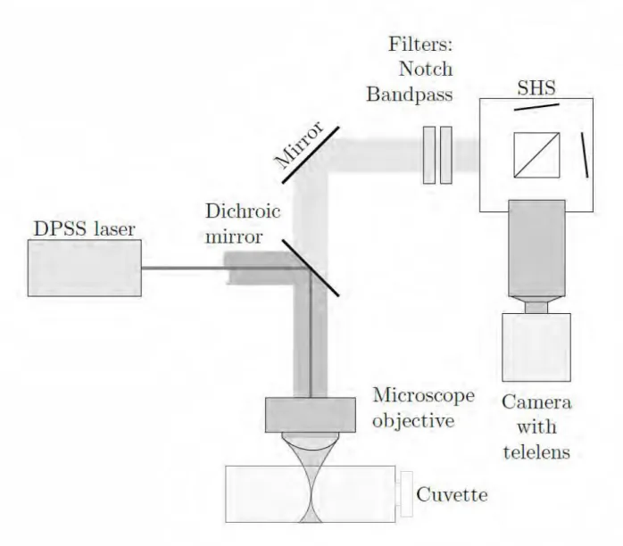
The experimental setup is shown in Figure 1 and theoretical details are available in the Appendix. The setup was configured in the collinear (backscatter) geometry. The laser was a diode-pumped solid-state laser (DPSS, Conqueror 25 W all-in-one, Compact Laser Solutions) operated at 532 nm with the pulse energy up to 100 µJ, pulse duration 20 ns, and repetition rate up to 80 kHz. A dichroic mirror (Semrock, RazorEdge Dichroic Beamsplitter 532) reflected the laser light into a microscope objective. The mirror was transparent at wavelengths longer than 532 nm thereby allowing the observation of Stokes Raman backscattering. A liquid sample was put in a quartz cuvette (a 10 x 10 x 50 mm3 spectrophotometer cell) which was positioned horizontally with its longest face perpendicular to the laser beam. The laser was focused inside the cuvette by a 10x microscope objective with the focal length 20 mm and entrance aperture 9 mm (Thorlabs LMH-10x-532). The same objective was used to collect the Raman signal. The numerical aperture of the objective was 0.25 and the collection solid angle 0.2 sr. The Raman scattered light was collimated by the objective, passed through the dichroic mirror, and was directed to the SHS. The notch (Semrock NF01-532U-25) and bandpass (LOT, 550+/–25 nm) filters were placed in front of the SHS to block the laser light and broadband fluorescence emitted by a sample. A cube beam splitter (Thorlabs BS013, 25 mm) was used to split the light 50/50 between the two arms of the SHS terminated by the diffraction gratings (Newport
33010FL01-270R, 50x50 mm2, 300 mm–1). The gratings were set at a Littrow angle θ ≈ 4.78o for the wavelength λL= 555 nm thus assuring the laser line at 532 nm to be close to the lower (blue) end of the spectral range. This allowed only the Stokes part of the Raman spectrum to be recorded. With these gratings, the resolving power 𝑅 = 5400 (δσ = 3.3 cm−1) at λ = 555 nm was calculated using Eq. A8, Appendix. The bandwidth was 2300 cm−1 (or 71 nm) calculated from Eq. A7, Appendix. This was sufficient to detect the Raman bands of molecules of interest.
The light dispersed by the gratings recombined at the beam splitter and created Fizeau
interference fringes. The fringes were imaged onto a CCD (Retiga R1, 1376x1024 pixels, 6.5 x 6.5 µm2 pixel pitch) by a Tamron telelens (focal distance 300 mm). The spectral response of the
camera was almost flat in the range 500 nm–600 nm with the quantum efficiency 70–75%. The etendue of the system, i.e., the largest beam diameter the SHS can accept, was limited by the 9 mm entrance aperture of the microscope objective. The camera was operated under the
µManager software.28,29 Three images were sequentially collected to create interferograms with the highest possible contrast: one with unblocked gratings and two with one of the gratings sequentially blocked. Two latter images were subtracted from the first one thus allowing the additional rejection of stray light and improving the quality of the interferogram. The optical elements and the detector camera were placed on a breadboard and enclosed into a black housing for shielding the instrument from ambient light.
Samples
Samples for Raman quantitative analysis, cyclohexane, isopropanol, and glycerol were chosen for the following reasons. Cyclohexane is often used as a reference standard in Raman
spectroscopy30 while isopropanol is miscible in cyclohexane and has a rich Raman spectrum that can be compared to that of cyclohexane. The cyclohexane–isopropanol mixture was therefore chosen to test the ability of the SHS–Raman instrument for quantitative analysis. Glycerol is a common substance in food and pharmaceutical industries; measuring its content in aqueous solutions is important to assess the products quality. For example, fermentation of wine was monitored by detecting its glycerol content.31
Cylohexane (ChemSolute, min 99.8% C6H12) and isopropanol (2-propanol, ChemSolute, min 99.8% CH3CH(OH)CH3) were volumetrically mixed to obtain 15 standard solutions with concentrations 0, 2, 4, 6, 8, 10, 25, 50, 75, 90, 92, 94, 96, 98, and 100 vol%. Because the densities of cyclohexane and isopropanol are close32 (0.7739 g cm–3 and 0.7809 g cm–3,
correspondingly), the volumetric and mass concentrations are nearly the same.Seven aliquots of Glycerol (Sigma-Aldrich, min 99.5% GC) were weighed and mixed with water (Milli-Q,
Millipore Synthesis A10) to produce standard solutions with concentrations of glycerol 0.1, 0.2, 0.5, 1, 2.5, 5 and 10 mass%.
Samples for classification, industrial oils, were chosen for a demand in a portable instrument that would be capable of fast identification of oil and oil spills in environmental and industrial areas.33 Six oil samples were biodiesel, poly(1-decene), gasoline, heavy oil IFO380,
polybutenes and lubricant. Biodiesel and heavy oil IFO380 were collected from the oil spill at Donges refinery (France), lubricant (Liqui Moly 10W-40) and gasoline were purchased at a gas station, and poly(1-decene) and polybutenes were purchased from Sigma-Aldrich. Biodiesel mainly consists of fatty acid methyl esters (FAME), generally produced by transesterification of vegetable oils and animal fats.34 Poly(1-decene), [CH2CH[(CH2)7CH3]]n, is a polymer that belongs to the class of poly-alpha-olephins and can be a product of the mineral oil pyrolysis.35 Gasoline, a fuel for the internal combustion engines, has a typical composition of 4–8% alkanes;
2–5% alkenes; 25–40% isoalkanes; 3–7% cycloalkanes; l–4% cycloalkenes; and 20–50% total aromatics (0.5–2.5% benzene).36 The heavy oil IFO 380 is a mix of 98% of residual oil and 2%
of distillate oil; it serves a fuel for very large compression ignition engines, such as oceangoing ships.37 Polybutenes are straight chain, aliphatic polymers made up of predominantly the
isobutylene repeat unit.38 The lubricant oil is a balanced mix of base oils and additives, e.g., zinc dialkyl dithiophosphates, molybdenum disulfide, and similar compounds, that determine its behavior both in terms of performance and duration.39,40
Image Processing
A typical SHS interferogram is the superposition of the modulated signal (interference fringes) and unmodulated background. The background is produced by stray light and light coming from out-of-phase parts of crossing wave fronts (Figure A1, Appendix). Several techniques can be used to improve the contrast of interferograms and quality of FFT-reconstructed spectra. These are the flat-field and phase corrections and apodization. In our experiment, the background due to the stray and out-of-phase light was removed by subtracting two auxiliary images from the interferogram. The auxiliary images were those obtained with one of the SHS arms blocked. The resulting intensity after the subtraction is
𝐼 = (𝐼s− 𝐼d) − [(𝐼a1− 𝐼d) + (𝐼a2− 𝐼d)] (1)
where 𝐼s is the pixel intensity on the original interferogram, 𝐼a1 and 𝐼a2 are the pixel intensities on the auxiliary images with one arm, a1 or a2, opened and other blocked, and 𝐼d is the pixel intensity on the dark image (the pixel index is omitted for better readability). The alternative flat- field correction via 𝐼 = (𝐼s− 𝐼d)/(𝐼a1+ 𝐼a2 − 2𝐼d) was unnecessary as it did not improve the
quality of interferograms but produced artifacts around zero frequency of FFT. The apodization (i.e., smoothing ripples due to FFT) was also unnecessary because reconstructed spectra were sufficiently smooth.
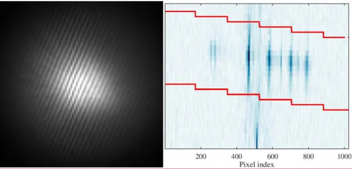
Figure 2 shows the interferogram from cyclohexane (a) and the 2D spectrum
reconstructed from it (b). Only the 1024 × 14 pixel region squeezed between two broken lines in Figure 2b contains useful information. Pixels within this region are vertically binned to produce intensity versus Raman shift spectrum. The downward drift of the lines with the increase of the pixel number is due to a slight tilt of the diffraction gratings about the x-axis (see Fig. A1, Appendix). The tilt removes ambiguity in identification of lines with equal positive and negative shifts with respect to the Littrow wavelength and thus effectively doubles the spectral range4. All images are processed with the GNU Octave software using the built-in fft2 function.41,42 The applicability of the code is tested using synthetic interferograms.
Calibration of SHS
Initial alignment of the SHS was done with a tungsten lamp by putting the line of zero path difference (ZPD) (Figure A1 in Appendix) in the center of the CCD pixel array. The wavelength calibration was carried out using the DPSS laser and the mercury lamp (Ocean Optics HG-1) following the procedure by Englert et al.43 The result of the calibration was a relationship between the pixel number on the SHS spectrum and the wavelength (or wavenumber) of a Raman band reconstructed from the interferogram. Raman spectra of acetone, ethanol, methanol, cyclohexane, and isopropanol were used to test the accuracy of the calibration; they are shown in Figure 3. The positions of Raman bands in Figure 3 coincide with the corresponding Raman shifts given in the AIST Database.44
Results and Discussion Performance of SHS
The actual resolving power of the instrument was evaluated using the narrow line of cyclohexane at 803 cm−1 which has the full width at half maximum (FWHM) 6 cm–1. Assuming the Gaussian shape for this line and using the Rayleigh criterion, the estimated resolution of the SHS is
estimated to be δσ = 4 cm−1 or 𝑅 = (λ ∙ δσ)−1 = 5000. This is 8% worse than the resolution predicted theoretically (𝑅 = 5400) that can be explained by the limited temporal coherence of
the interfering wave packets24. As the overall intensity decreases toward the edges of the
interferogram (Figure 2a), the kernel of the FFT integral acquires an effective (nearly triangular) weight function. This results in further broadening of the FFT-reconstructed spectral lines and thus further deteriorates the resolution. We note, however, that the highest possible spectral resolution was not the goal; the bands of interest were clearly seen and resolved.
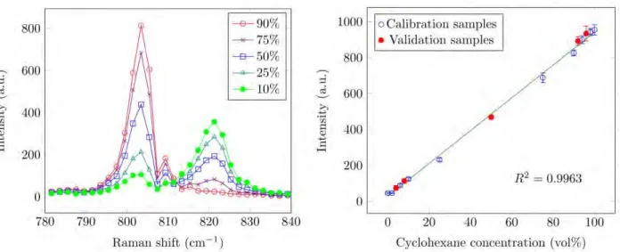
Next, the adequacy of a linear calibration model for determination of cyclohexane in isopropanol was tested. The Raman spectra of cyclohexane in isopropanol were baseline- subtracted (using the algorithm proposed by Gan et al.45) and corrected for a spectral response function (the dashed line in Figure 3a). Several Raman spectra corresponding to different concentrations of cyclohexane in isopropanol are shown in Figure 4a. The integral intensities of the cyclohexane (803 cm–1) and isopropanol (820 cm–1) bands were normalized to their
corresponding concentrations and rationed. Table I shows the normalized intensity ratios for several concentrations of cyclohexane in isopropanol. The average intensity ratio 2.69 ± 0.20, which was calculated using the data in the last column of Table I, is close to the ratio 2.79 of the Raman cross-sections of the bands, 4.55 ∙ 10−30 cm−2 and 1.63 ∙ 10−30 cm−2, correpondingly46. This proves that the Raman signals are approximately proportional to concentrations, at least within the range of 10–90 vol% of cyclohexane in isopropanol. The adequacy of the linear calibration model is thus confirmed.
Quantitative Analysis of Organic Solutions Cyclohexane in Isopropanol
Two calibration techniques, univariate and multivariate via PLSR, were used to quantify cyclohexane in isopropanol. First, the univariate method was applied. Ten out of fifteen sample sets were used for calibration and five (4, 8, 50, 92, 96 vol %) for validation. Each set consisted of ten measurements. A spectral fragment between 780 cm−1 and 840 cm−1 was chosen. Figure 4a shows the Raman spectra of cyclohexane and isopropanol for several selected concentrations.
The integral intensity of the 803 cm−1 cyclohexane band was the analytical signal. The
calibration plot is displayed in Figure 4b; error bars are the standard deviations over 10 repetitive measurements.
The overall accuracy of the analysis is assessed by the root mean square error of cross validation (RMSECV%) and prediction (RMSEP%) normalized to the concentration range
𝑅𝑀𝑆𝐸% = 100
𝑦max−𝑦min√Σ𝑖=1𝑛 (𝑦𝑖−𝑦̂ )𝑖 2
𝑛 (2)
where 𝑦𝑖 and 𝑦̂𝑖 are the certified and found concentrations related to the calibration (n=100) or the validation (n=50) sets, and 𝑦max− 𝑦min is the concentration range spanned by the sets. The metric expressed by Eq. 2 allows for a direct comparison of different spectroscopic methods that deal with different ranges of concentrations.
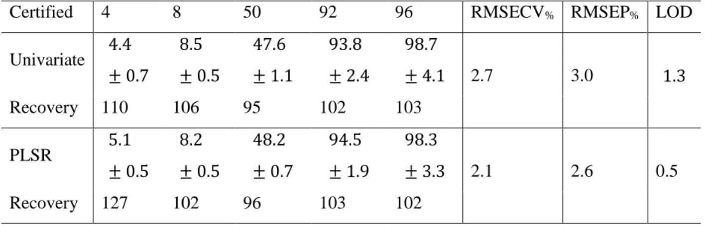
The results of the univariate quantitative analysis are summarized in the middle row of Table II. The RMSECV% and RMSEP% are 2.7% and 3.0% for the concentration ranges 2–100%
and 4–96%, correspondingly. The low values of the relative errors along with the high value of the coefficient of determination (𝑅2= 0.9963) confirm the high overall accuracy of the calibration and analysis. Values for the recovery are between 95% and 110% for the validation set. The relative standard deviation of the determination (precision) varies between 6% and 16%
for low concentrations (<10%) and between 2% and 4% for high concentrations (>10%). The limit of detection (LOD) is 1.3% based on the 3σ criterion.
We also performed multivariate PLSR analysis of cyclohexane in isopropanol to possibly improve figures of merit. The calibration and validation sets were the same as in the univariate analysis. Two principal components (PC) were found to be optimal based on the minimal value of PRESS (predicted residual sum of squares) determined by the leave-one-out cross-validation.
The results of PLSR analysis are shown in the last two rows of Table II. One infers from the table that both the RMSECV% and RMSEP% are indeed lower as compared to the univariate analysis. The LOD is also lower and decreases from 1.3% (univariate) to 0.5% (PLSR).
However, the overall accuracy of analysis remains the same as seen from the values of recoveries. The recovery is even worse for the lowest determined concentration (4%), 127%
(PLSR) versus 110% (univariate). We thus conclude that both the methods are suitable for quantification and perform similarly.
Glycerol in Water
Analysis of glycerol in water is more challenging because glycerol exhibits only weak Raman peaks. This makes SHS measurements difficult because signal-to-noise ratios are low at
intermediate and low concentrations. Raman spectra of glycerol in water are shown in Figure 5a.
One sees that glycerol bands47 at 485, 850, and 1052 cm–1 are barely visible as concentration of glycerol falls below 5%. This makes univariate analysis difficult. On the other hand, multivariate analysis remains apt as it reveals latent properties of spectral data such as the hidden variation of spectra with concentrations.
Six samples (0.1, 0.2, 0.5, 5, and 10%) were used for calibration and two (1 and 2.5%) for validation. Prior to PLSR, the baseline was removed and spectra were smoothed using a soft, 15 points, second polynomial, Savitzky–Golay filter. Four PCs were used based on the minimal value of PRESS. The accuracy of the calibration and analysis are assessed by the values of RMSECV% and RSMEP% that were 3.8% and 21.2% for the concentration ranges 0.1–10% and 1–2.5%, correspondingly.
The certified-found plot is shown in Figure 5b. The predicted concentrations of the two tested samples were somewhat overestimated at (1.4 ± 0.2)% and (2.7 ± 0.2)% with the values for the recovery 140% and 108%, correspondingly. The LOD was found to be 0.5%, the same as for cyclohexane in isopropanol.
The results obtained with SHS are comparable with that obtained by other Raman techniques. For example, Schweinsberg et al.48 used a commercial FT Raman spectrometer to determine cyclohexane in toluene in the concentration range 13–96%. The relative error of the linear regression model was 0.7% with the 100–104% recovery. McCain et al.49 constructed a coded-aperture Raman spectrometer in which the input slit of the dispersive spectrograph was replaced by the 2D mask. The intensity pattern, a convolution of the Raman spectrum with the input aperture, was detected by a 2D detector and then reconstructed to produce the original Raman spectrum. Concentrations of ethanol in tissue-like phantoms were determined in the concentration range 0.04–0.8 mass% using PLSR with RMSEP% below 3.5%. Voss et al.50 reported the measurement of glycerol, methanol, ammonia, and secreted protein in biological samples (cell culture broth) using a commercial Raman instrument with a dispersive
spectrometer. Glycerol was measured in the concentration range 0.2 to 5% using the multivariate techniques PLSR and Support Vector Regression (SVR). The RMSEP% for glycerol determined using PLSR was 3.5%.
Discrimination of Oils
Fingerprinting and source identification of oil spills is an important problem in environmental and industrial forensics.51 Accidental spills and intentional discharges of petroleum products in waters and soils are frequent around the world. Typically, chemical fingerprinting is done using GC and GC-MS methods or by optical (UV–Vis–IR) and chemical sensors if remote analysis is needed. Using Raman spectroscopy for fingerprinting of petroleum products is a challenge because the complex composition of these products may result in ambiguous Raman spectra or no Raman spectra at all and/or a broadband fluorescence. Additives in oils produce strong fluorescence, which is the major challenge for obtaining SHS interferograms with good fringe contrast.
The goal of this test was to discriminate between petroleum products rather than to precisely identify them. The spectral information, both Raman and fluorescence, was so sample- specific that a simple unsupervised technique like principal component analysis (PCA) was sufficient to discriminate the samples. The specificity of spectral information can be appreciated from Figure 6a where the SHS spectra of oils are shown. Only two out of six samples exhibit distinct Raman spectra, polybutenes and poly(1-decene). The other samples exhibit mainly the broadband fluorescence spectra. The spectra were collected using a 60 s integration time for gasoline, poly(1-decene) and polybutenes, 10 s for IFO380, and 0.1 s for the lubricant. The Raman bands at 720, 897, 923, and 1217 cm–1 are characteristic for polybutenes and the bands at 868, 1055, 1303, and 1442 cm–1 are characteristic for poly(1-decene). Several bands were clearly identified, for example, C–C stretching in –(CH2)n– at 868 cm–1, C–H twisting in –CH2 at 1303 cm–1, and C–H scissoring in –CH2 at 1442 cm–1. The simple visual inspection of the spectra in Figure 6a is already sufficient to distinguish the oils from each other. Processing these data with PCA assures their reliable identification.
Figure 6b shows the results of PCA analysis. The first three principal components explain 97.5% of the variation in the data. One sees that PCA produces clearly distinguishable clusters;
the ratio of the shortest distance between cluster centers and the largest radius of a cluster is about three.
The classification results obtained by SHS are positively compared with the results obtained by other Raman techniques. El-Abassy et al.52 used a home-built dispersive Raman spectrometer to collect Raman spectra from pure olive oils and olive oils adulterated by sunflower oil. The PCA had successfully distinguished the adulterated samples even with the
smallest <5% addition of sunflower oil. Baeten et al.53 employed a FT–Raman spectrometer for the same purpose of discriminating between pure and adulterated olive oils using PCA. It was possible to discriminate clearly between genuine and 1% spiked samples. Jentzsch et al.54 used a handheld Raman spectrometer for the distinction of oils used in the cosmetic industry. The Raman spectra of oils were also clustered into distinct groups by PCA.
Conclusion
This study demonstrated the applicability of the SHS in combination with a DPSS laser for both qualitative and quantitative Raman spectroscopy of liquid samples and for sample classification.
A Raman SHS instrument was constructed and characterized. The spectrometer exhibited the resolving power of 5000 and spectral range of 520–590 nm. Raman shifts between 330 cm–1 and 1600 cm–1 could be measured.
Quantitative Raman analysis was performed for the first time using this technique. Two calibration methods, univariate and multivariate (PLSR) were used to determine cyclohexane in isopropanol in concentration range 2–100%. Both the methods yielded similar accuracy and precision of analysis; the LODs were 1.3% and 0.5%, correspondingly. Only multivariate PLSR analysis was carried out for glycerol in water in the concentration range 0.1–10%; it yielded the overestimated by 40% and 8% values for the two determined concentrations; the LOD was 0.5%.
Six industrial oils, biodiesel, poly1-decene, gasoline, heavy oil IFO380, polybutenes, and lubricant were discriminated by means of PCA using their Raman–fluorescence spectra. Albeit the additives in oils produced strong fluorescence that deteriorated the contrast of SHS
interferograms, all oils showed distinct non-overlapping clusters in the principal component space. The distance between the clusters was about three times the largest cluster dimension.
This was a test for the applicability of SHS for materials discrimination based on their Raman/fluorescence spectra. In the future, given a library of oil spectra, a supervised
classification can be done that will allow for not only discrimination but classification of oils and other organic materials.
Acknowledgements
D.P. and G.G. acknowledge the financial support received from various sources including the Ministry of Human Capacities (through project 20391-3/2018/FEKUSTRAT) and the National
Research, Development and Innovation Office (through projects K129063 and EFOP-3.6.2-16- 2017-00005 “Ultrafast Physical Processes in Atoms, Molecules, Nanostructures, and Biological Systems”) of Hungary. A.B.G. thanks Dr. Andreas Bierstedt (BAM) for his help with Raman instrumentation, Mr. Lukas Wander (BAM) for providing glycerol samples, and Dr. Maria Mansurova (BAM, Qioptiq) for providing oil samples.
References
1. A. Thorne, U. Litzen, S. Johansson. “Spectrophysics: Principles and Applications”. Berlin:
Springer, 1999. Pp. 334–336.
2. J. Connes. “Domaine d’Utilisation de la Méthode par Transformée de Fourier”. J. Phys.
Radium. 1958. 19(3): 197–208.
3. T. Dohi, T. Suzuki. “Attainment of High Resolution Holographic Fourier Transform Spectroscopy”. Appl. Opt. 1971. 10(5): 1137–1140.
4. J.M. Harlander. “Spatial Heterodyne Spectroscopy: Interferometric Performance at any Wavelength Without Scanning”. [Doctor of Philosophy Dissertation]. United States of America: University of Wisconsin–Madison, 1991.
5. J.M. Harlander, R.J. Reynolds, F.L. Roesler. "Spatial Heterodyne Spectroscopy for the Exploration of Diffuse Interstellar Emission Lines at Far-Ultraviolet Wavelengths”.
Astrophys. J. 1992. 396(2): 730–740.
6. N.G. Douglas. "Heterodyned Holographic Spectroscopy”. Publ. Astron. Soc. Pac. 1997.
109(732): 151–165.
7. O.R. Dawson, W.M. Harris. “Tunable, All-Reflective Spatial Heterodyne Spectrometer for Broadband Spectral Line Studies in the Visible and Near-Ultraviolet”. Appl. Opt. 2009.
48(21): 4227–4238.
8. S. Hosseini. “Characterization of Cyclical Spatial Heterodyne Spectrometers for Astrophysical and Planetary Studies”. Appl. Opt. 2019. 58(9): 2311–2319.
9. T. Nathaniel. “Spatial Heterodyne Raman Spectroscopy”. [Doctor of Philosophy Dissertation].
UK: Univ. of Surrey, 2011.
10. N.R. Gomer, C.M. Gordon, P. Lucey, S.K. Sharma, et al. “Raman Spectroscopy Using a Spatial Heterodyne Spectrometer: Proof of Concept”. Appl. Spectrosc. 2011. 65(8): 849–
857.
11. I.B. Gornushkin, B.W. Smith, U. Panne, N. Omenetto. "Laser-Induced Breakdown
Spectroscopy Combined with Spatial Heterodyne Spectroscopy”. Appl. Spectrosc. 2014.
68(9): 1076–1084.
12. P.D. Barnett, N. Lamsal, S.M. Angel. “Standoff Laser-Induced Breakdown Spectroscopy (LIBS) Using a Miniature Wide Field of View Spatial Heterodyne Spectrometer with Sub-Microsteradian Collection Optics”. Appl. Spectrosc. 2017. 71(4): 583–590.
13. J.A. Langille, D. Letros, D. Zawada, A. Bourassa, et al. Spatial Heterodyne Observations of Water (SHOW) Vapour in the Upper Troposphere and Lower Stratosphere from a High Altitude Aircraft: Modelling and Sensitivity Analysis”. J. Quant. Spectrosc. Radiat.
Transfer. 2018. 209: 137–149.
14. M.W. Kudenov, M.N. Miskiewicz, M.J. Escuti, E.L. Dereniak. “Spatial Heterodyne Interferometry with Polarization Gratings”. Opt. Lett. 2012. 37(21): 4413–4415.
15. J. Qiu, X. Qi, X. Li, Z. Ma, et al. “Development of a Spatial Heterodyne Raman
Spectrometer with Echelle-Mirror Structure”. Opt. Express. 2018. 26(9): 11994–12006.
16. P.D. Barnett, S.M. Angel. “Miniature Spatial Heterodyne Raman Spectrometer with a Cell Phone Camera Detector. Appl. Spectrosc. 2017. 71(5): 988–995.
17. J. Qiu, X. Qi, X. Li, Y. Tang, et al. “Broadband Transmission Raman Measurements Using a Field-Widened Spatial Heterodyne Raman Spectrometer with Mosaic Grating Structure”.
Opt. Express. 2018. 26(20): 26106–26119.
18. J. Liu, Bayanheshig, X. Qi, S. Zhang, et al. “Backscattering Raman Spectroscopy Using Multi-Grating Spatial Heterodyne Raman Spectrometer”. Appl. Opt. 2018. 57(33): 9735–
9745.
19. C.R. Englert, J.M. Harlander. “Flatfielding in Spatial Heterodyne Spectroscopy”. Appl. Opt.
2006. 45(19): 4583–4590.
20. C.R. Englert, J.M. Harlander, J.G. Cardon, F.L. Roesler. “Correction of Phase Distortion in Spatial Heterodyne Spectroscopy”. Appl. Opt. 2004. 43(36): 6680–6687.
21. M.J. Egan, S.M. Angel, S.K. Sharma. “Optimizing Data Reduction Procedures in Spatial Heterodyne Raman Spectroscopy with Applications to Planetary Surface Analogs”. Appl.
Spectrosc. 2018. 72(6): 933–942.
22. J. Liu, D. Wei, O. Wroblowski, Q. Chen, et al. “Analysis and Correction of Distortions in a Spatial Heterodyne Spectrometer System”. Appl. Opt. 2019. 58(9): 2190–2197.
23. B.J. Cooke, B.W. Smith, B.E. Laubscher, P.V. Villneuve, et al. “Analysis and System Design Framework for Infrared Spatial Heterodyne Spectrometers”. Proceedings Infrared
Imaging Systems: Design, Analysis, Modeling, and Testing X. 3701. 1999. DOI:
10.1117/12.352971.
24. M. Lenzner, J.-C. Diels. "Concerning the Spatial Heterodyne Spectrometer”. Opt. Express.
2016. 24(2): 1829–1839.
25. C.P. Perkins, J.P. Kerkes, M.G. Gartley. “Spatial Heterodyne Spectrometer: Modeling and Interferogram Processing for Calibrated Spectral Radiance Measurements”. Proc. SPIE 8870. 2013. DOI: 10.1117/12.2023765.
26. M.J. Egan, S.M. Angel, S.K. Sharma. “Standoff Spatial Heterodyne Raman Spectrometer for Mineralogical Analysis”. J. Raman Spectrosc. 2017. 48(11): 1613–1617.
27. T. Jawhari, P.J. Hendra, H.A. Willis, M. Judkins. “Quantitative Analysis Using Raman Methods”. Spectrochim. Acta, Part A. 1990. 46(2): 161–170.
28. C.A. Schneider, W.S. Rasband, K.W. Eliceiri. “NIH Image to ImageJ: 25 Years of Image Analysis”. Nat. Methods. 2012. 9(7): 671–675.
29. A.D. Edelstein, M.A. Tsuchida, N. Amodaj, H. Pinkard, et al. “Advanced Methods of Microscope Control Using µManager Software”. J. Bio. Methods. 2014. 1(2): e10.
30. R.L. McCreery. Raman Spectroscopy for Chemical Analysis. New York: Wiley, 2000.
31. Q. Wang, Z. Li, Z. Ma, L. Liang. "Real Time Monitoring of Multiple Components in Wine Fermentation Using an On-Line Auto-Calibration Raman Spectroscopy”. Sens.
Actuators, B. 2014. 202: 426–432.
32. D.R. Lide. “Physical Constants of Organic Compounds”. Boca Raton, FL: CRC Handbook of Chemistry and Physics, 2003. Section 3.
33. S. Johann, M. Mansurova, H. Kohlhoff, A. Gkertsos, et al. “Wireless Mobile Sensor Device for In-Situ Measurements with Multiple Fluorescent Sensors”. Paper presented at: 2018 IEEE Sensors. New Delhi, India; 28–31 October 2018. DOI:
10.1109/ICSENS.2018.8589666.
34. S.K. Hoekman, A. Broch, C. Robbins, E. Ceniceros, et al. “Review of Biodiesel
Composition, Properties, and Specifications”. Renewable Sustainable Energy Rev. 2012.
16(1): 143–169.
35. P. Kusch, V. Obst, D. Schroeder-Obst, W. Fink, et al. “Application of Pyrolysis-Gas Chromatography/Mass Spectrometry for the Identification of Polymeric Materials in Failure Analysis in the Automotive Industry”. Eng. Failure Anal. 2013. 35: 114–124.
36 C. Harper, J.J. Liccione. “Toxicological Profile for Automotive Gasoline”. Atlanta: Agency for Toxic Substances and Disease Registry (ATSDR), 1995. Pp. 107.
37. A. Friedrich, F. Heinen, F. Kamakate, D. Kodjak. ”Air Pollution and Greenhouse Gas Emissions from Ocean-Going Ships: Impacts, Mitigation Options and Opportunities for Managing Growth”: Washington: The International Council on Clean Transportation (ICCT), 2007. Pp. 48.
38. M. Casserino, J. Corthouts. “Polybutenes”. In L.R. Rudnick, editor. Synthesis, Mineral Oils, and Bio-Based Lubricants. Boca Raton: CRC Press, 2nd ed. 2013. Pp. 273–301.
39. B.C. Windom, W.G. Sawyer, D.H. Hahn. “A Raman Spectroscopic Study of MoS2 and MoO3: Applications to Tribological Systems”. Tribol. Lett. 2011. 42(3): 301–310.
40. X. Xia, A. Morina, A. Neville, M. Priest, et al. “Tribological Performance of an Al–Si Alloy Lubricated in the Boundary Regime with Zinc Dialkyldithiophosphate and Molybdenum Dithiocarbamate Additives”. Proc. Inst. Mech. Eng., Part J. 2008. 222(3): 305–314.
41. J.W. Eaton, D. Bateman, S. Hauberg, R. Wehbring. “GNU Octave Version 4.2.0 Manual: A High-Level Interactive Language for Numerical Computing”. http:
//www.gnu.org/software/octave/doc/interpreter/ [accessed Jun 25 2019].
42. D.G. Voelz. “Computational Fourier Optics: A MATLAB Tutorial”. Bellingham: SPIE Press, 2011. Chap. 2, Pp. 29–45.
43. C.R. Englert, J.M. Harlander, J.C. Owrutsky, J.T. Bays. “SHIM-Free Breadboard Instrument Design, Integration, and First Measurements”. NRL/MR/7640-05-8926, Washington DC:
Naval Research Laboratory Defense Technical Information Center, 2005. https:
//apps.dtic.mil/docs/citations/ADA441898 [accessed Jun 25 2019].
44. T. Saito, T. Yamaji, K. Hayamizu, M. Yanagisawa, et al. Spectral Database for Organic Compounds SDBS. Japan: National Institute of Advanced Industrial Science and Technology. https: //sdbs.db.aist.go.jp [accessed Jun 25 2019].
45. F. Gan, G. Ruan, J. Mo. “Baseline Correction by Improved Iterative Polynomial Fitting with Automatic Threshold”. Chemom. Intell. Lab. Syst. 2006. 82(1–2): 59–65.
46 T.E. Acosta-Maeda, A.K. Misra, J.N. Porter, D.E. Bates, et al. “Remote Raman Efficiencies and Cross-Sections of Organic and Inorganic Chemicals”. Appl. Spectrosc. 2017. 71(5):
1025–1038.
47. E. Mendelovici, L.F. Ray, T. Kloprogge. “Cryogenic Raman Spectroscopy of Glycerol”. J.
Raman Spectrosc. 2000. 31(12): 1121–1126.
48. D.P. Schweinsberg, Y.D. West. “Quantitative FT Raman Analysis of Two Component Systems”. Spectrochim. Acta, Part A. 1997. 53(1): 25–34.
49. S.T. McCain, M.E. Gehm, Y. Wang, N.P. Pitsianis, et al. “Coded Aperture Raman Spectroscopy for Quantitative Measurements of Ethanol in a Tissue Phantom”. Appl.
Spectrosc. 2006. 60(6): 663–671.
50. J.-P. Voss, N.E. Mittelheuser, R. Lemke, R. Luttmann. “Advanced Monitoring and Control of Pharmaceutical Production Processes with Pichia Pastoris by Using Raman
Spectroscopy and Multivariate Calibration Methods”. Eng. Life Sci. 2017. 17(12): 1281–
1294.
51. S. Stout, Z. Wang. "Chemical Fingerprinting of Spilled or Discharged Petroleum – Methods and Factors Affecting Petroleum Fingerprints in the Environment”. Oil Spill
Environmental Forensics: Fingerprinting and Source Identification. Burlington:
Academic Press, 2007. Chap. 1, Pp. 1–53.
52. R.M. El-Abassy, P. Donfack, A. Materny. “Visible Raman Spectroscopy for the Discrimination of Olive Oils from Different Vegetable Oils and the Detection of Adulteration”. J. Raman Spectrosc. 2009. 40(9): 1284–1289.
53. V. Baeten, R. Aparicio. “Edible Oils and Fats Authentication by Fourier Transform Raman Spectrometry”. Biotechnol., Agron., Soc. Environ. 2000. 4(4): 196–203.
54. P.V. Jentzsch, L.A. Ramos, V. Ciobota. “Handheld Raman Spectroscopy for the Distinction of Essential Oils Used in the Cosmetics Industry”. Cosmetics. 2015. 2(2): 162–176.
Appendix
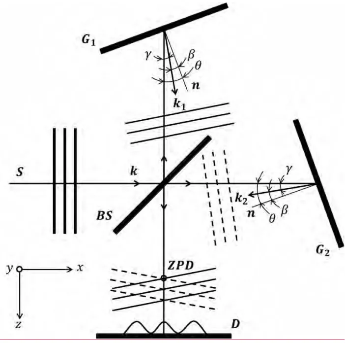
The basic operational principle of SHS is illustrated in Figure A1. We limit our discussion to the situation when collimated light from a light source propagates along the SHS optical axis so that the angles of incidence and diffraction for the two SHS gratings are the same for the same wavelengths (wavenumbers). A more elaborate treatment of SHS operational modes can be
found elsewhere.4,10,11 Let the origin of the coordinate system be at a center of the beam splitter, the 𝑧-axis be aligned with the detector optical axis, the 𝑦-axis be perpendicular to the image plane and parallel to the gratings grooves, and the 𝑥-axis be in the image plane. Let the plane incident wave with the wave vector 𝐤 propagate along the x-axis. After splitting, the two partial waves diffract on gratings G1 and G2 according to
σ(sin θ + sin β) = 𝑚/𝑑 (A1)
where σ = 1/λ is the wavenumber, m and d are the diffraction order and the groove spacing, θ and β are the angles of incidence and diffraction (equal for both the gratings).
The gratings are tilted to a small angle (typically several degrees) with respect to the optical axis to provide a Littrow condition (angle of incidence = angle of diffraction) for a chosen wavenumber σ0: 2 sin θ = 𝑚/𝑑σ0, or 𝑚 = 2𝑑σ0sin θ. The diffracted waves with the wave vectors 𝐤𝟏 and 𝐤𝟐 (|𝐤𝟏| = |𝐤𝟐| = 2πσ) recombine at the beam splitter and create the interference pattern
𝐼 = 𝐼1+ 𝐼2 + 2√𝐼1𝐼2cos[𝐫 ∙ (𝐤𝟐− 𝐤𝟏)] = 𝐼0(1 + cos[𝐫 ∙ (𝐤𝟐− 𝐤𝟏)]) (A2)
where 𝒓 is the radius-vector and 𝐼1 = 𝐼2 = 𝐼0/2. Assuming the plane waves to be strictly parallel to the 𝑦-axis, the three coordinate components of the diffracted waves are (|𝐤𝟏| cos γ, 0, −
|𝐤𝟏| sin γ) and (|𝐤𝟐| cos γ, 0, |𝐤𝟐| sin γ) where γ = β − θ is the angle between the diffracted wave vector and the optical axis (𝑥 or 𝑧). The angle γ is counted counterclockwise from the 𝑥- axis. This angle can easily be found from the diffraction Eq. A1 by the simple substitutions β = θ − γ and 𝑚 = 2𝑑σ0sin θ and using the trigonometric equation for the sine of the difference of two angles:
γ = 2σ−σ0
σ tan θ (A3)
For small angles γ, the dot product in Eq. 5 is 𝐫 ∙ (𝐤𝟐− 𝐤𝟏) = 2πσ[𝑥 (sin γ + sin γ) + 𝑧 (cos γ − cos γ)] ≈ 4πσ𝑥𝛾. Substituting this and Eq. A3 into Eq. A2 obtains
𝐼(𝑥) = 𝐼0(1 + cos[ 2π ∙ 4𝑥 ∙ (σ − σ0) tan θ]) (A4)
For a polychromatic light source, Eq. A4 transforms into
𝐼(𝑥) = ∫ 𝐵(σ)(1 + cos[ 2π ∙ 4𝑥 ∙ (σ − σ0∞ 0) tan θ])𝑑σ (A5)
where 𝐵(σ) is the input spectrum and 𝐵(σ)𝑑σ is the intensity at σ. Three important conclusions can be drawn from Eq. A5. First, this is a Fourier transform of the input spectrum 𝐵(σ); second, the intensity is spatially (cosine-like) modulated along the x-axis; and third, the modulation frequency is heterodyned around the Littrow σ0. The heterodyning converts high oscillation frequencies on order 𝜎 into low differential frequencies on order (σ − σ0) thus making possible the detection of spatially modulated intensities (interferograms) with conventional array
detectors with pixel size of about 10 μm. The conversion of Eq. A5 back into the spectral domain is done by a Fourier transform of this equation using a suitable algorithm, e.g., the fast Fourier transform (FFT).
As deduced from Eq. A5 and the general definition of a periodic function, 𝑓(𝑥) = cos(ω𝑥), ω = 2π/𝑞, the interference fringes along the x-axis have the spatial period
𝑞 = 1/[4(σ − σ0) tan θ] (8)
Interference fringes are recorded by an image sensor having 𝑁 pixels along the 𝑥- direction, each pixel having size 𝑙 . Based on the Nyquist–Shannon sampling theorem, the smallest period that can be resolved is twice the pixel size, i.e., 𝑞min = 2𝑙. This means that for 𝑁 detector elements, only 𝑁/2 spectral elements can be recovered. Consequently, when an imaging system with the unit magnification is used, the largest wavenumber interval is found from Eq.
A7 by setting [4(σ − σ0) tan θ]max = 1/𝑞min = 1/2𝑙 and assigning Δσmax= σmax− σ0 :
Δσmax = 1/(8𝑙 tan θ) (A7)
This equation determines the unaliased bandwidth of the instrument.
The limiting resolving power of the instrument, 𝑅0 = σ/δσ is equal to the theoretical resolving power of the dispersive system and for the geometry in Figure A1 is
𝑅0 = 4𝑊σ sin θ (A8)
where W is the width of the grating that is imaged on the detector and θ is the Littrow angle. In practice, the resolving power is worse than that given by Eq. A8, mainly due to the limited temporal coherence of the interfering plane waves.24
Figure A1. Illustration of basic principle of SHS. 𝑆 is the light source, 𝐵𝑆 is the cube beam splitter, 𝐺1 and 𝐺2 are the gratins, n is the grating normal, tilted by the angle θ with regards to the optical axes, 𝐷 is the detector plane, and 𝑍𝑃𝐷 is the zero-path-difference line (this line is parallel to the grating grooves, i.e., the 𝑦-axis). Lenses that collimate the light from the source and image the interference fringes on the detector are not shown.
Tables
Table I. Ratios (𝑹) of normalized integral intensities of cyclohexane and isopropanol bands 𝟖𝟎𝟑 𝐜𝐦−𝟏 and 𝟖𝟐𝟎 𝐜𝐦−𝟏 corrected for respective concentrations for mixtures with
different proportions of cyclohexane and isopropanol.
𝐶cyc/𝐶iso 𝐼803/𝐶cyc 𝐼820/𝐶iso 𝑅
9/1 4.22 1.61 2.62
3/1 4.34 1.43 3.03
1/1 4.25 1.70 2.50
1/3 4.25 1.56 2.72
1/9 4.01 1.55 2.59
Table II. Results of univariate and multivariate analyses of cyclohexane in isopropanol (all
%).
Certified 4 8 50 92 96 RMSECV% RMSEP% LOD
Univariate 4.4
± 0.7 8.5
± 0.5
47.6
± 1.1
93.8
± 2.4
98.7
± 4.1 2.7 3.0 1.3
Recovery 110 106 95 102 103
PLSR 5.1
± 0.5 8.2
± 0.5
48.2
± 0.7
94.5
± 1.9
98.3
± 3.3 2.1 2.6 0.5
Recovery 127 102 96 103 102
Figure Captions
Figure 1. Experimental setup. Ray propagation inside SHS is given in Fig. A1, Appendix.
Figure 2. (a) SHS–Raman interferogram of cyclohexane; (b) FFT image of this interferogram.
Bounding lines define the region of interest containing useful information. Notice the line of zero frequency on the bottom, at pixel index 512.
Figure 3. (a) Raman spectra of acetone, ethanol and methanol. Spectra are shifted vertically for clarity and have a maximum signal to background noise ratio above 100. The dashed curve shows the combined transmittance of the bandpass and notch filters. (b) Raman spectra of the 1:3 mixture of cyclohexane and isopropanol. Raman bands of cyclohexane are 803, 1029, 1267, and 1445 cm–1, and isopropanol are 820, 955, 1132, and 1454 cm–1.
Figure 4. (a) Raman peaks of cyclohexane and isopropanol; the legend is concentrations of cyclohexane; (b) Calibration plot for cyclohexane in isopropanol.
Figure 5. (a) Raman spectra of glycerol in water for different concentrations. Each spectrum is the mean of ten baseline-corrected spectra. Spectra are shifted vertically for clarity. (b) Certified- found plot for glycerol in water constructed by accounting for 4 PCs in PLSR.
Figure 6. (a) Raman and fluorescent spectra of oils. (b) Scores plot from PCA of Raman spectra of oils for the first three components. The lines are the projections of the center point of the
group on the surface defined by the first two principal components.