Regional determinants of Hungarian wine prices: The role of geographical indications, objective quality and individual reputation

(1)

Wine Economics and Policy 10(1): 119-132, 2021

ISSN 2212-9774 (online) | ISSN 2213-3968 (print) | DOI: 10.36253/wep-8880

and Policy

Citation: Peter Gal, Attila Jambor, Sandor Kovacs (2021) Regional determinants of Hungarian wine prices:

The role of geographical indications, objective quality and individual reputa- tion. Wine Economics and Policy 10(1):

www.fupress.com/wep) and distributed under the terms of the Creative Com- mons Attribution License, which per- mits unrestricted use, distribution, and reproduction in any medium, provided the original author and source are credited.

Data Availability Statement: All rel- evant data are within the paper and its Supporting Information ﬁ les.

Competing Interests: The Author(s) declare(s) no conﬂ ict of interest.

Regional determinants of Hungarian wine prices: Th e role of geographical indications, objective quality and individual reputation

Peter Gal¹, Attila Jambor^1,*, Sandor Kovacs²

1 Corvinus University of Budapest, Hungary

2 University of Debrecen, Hungary

E-mail: peter.gal@stud.uni-corvinus.hu; attila.jambor@uni-corvinus.hu; kovacs.sandor@econ.unideb.hu

*Corresponding author.

Abstract. Analysing the determinants of wine prices has always been a fi eld of inter- est in the wine economics literature. By estimating hedonic price functions, however, most papers generally remain at the country level with regions generally neglected or treated as simple dummy variables. Th e aim of this paper is to analyse the determinants of wine prices at the regional level by using Latent Variable Path Modelling with Partial Least Squares and Principal Component Analysis on the example of Hungarian wines. Th is approach is able to capture the regional specialties of wine production and provides a better insight into price determination. Results suggest that intrinsic values play a major but ambiguous role in determining regional wine prices, especially in the case of sugar content. It also becomes apparent that specifi c Geographical Indications (GIs) play a crucial role in price determination, instead of GI use per se. Moreover, individual brands also have an important role, as Tier1 and Tier2 wineries tend to sell their wines at higher prices and in smaller batch sizes.

Keywords: wine regions, price determination, Hungary, quality, Partial Least Squares.

1. INTRODUCTION

A large amount of scientifi c literature has been dealing with the determinants of wine prices recently [1,2,3,4]. By mainly applying hedonic pricing models, the vast majority of these studies quantify the relationship between wine prices and, inter alia, origin, subjective and objective quality and labelling elements like variety, vintage or brands. Despite the large quantity of research into the topic, articles mainly focus on the country level and regions are oft en neglected or treated by simple dummy variables [5,6,7].

However, wine is a highly diff erentiated product and this diff erentiation starts at the regional level [5,8,9]. It largely depends on the regional characteristics of the kind of wine produced and such diversity is missed when wine prices are analysed at the country level. Th is article aims to analyse

(2)

the determinants of wine prices at the regional level by using Latent Variable Path Modelling with Partial Least Squares (LVPLS) and Principal Component Analy- sis (PCA), using the example of Hungarian wines. This approach is able to capture the regional specialties in wine production and provides a better insight into price determination. Our motivation to prefer this approach over the classical methods was based on some previous studies [10,11,12] using PLS and we followed the guidelines of Hair et al. [13].

The article is structured as follows. First, a literature review is given on the most important studies on the determinants of wine prices written between 1998 and 2018, and this is followed by a description of the methods and data used here. The third section shows our results together with a discussion, while the last part concludes.

2. GEOGRAPHICAL ORIGIN AS A DETERMINANT OF WINE PRICES

Origin has always been considered one of the most important determinants of wine prices. In this regard, a significant part of the literature analyses the role of geo- graphical indications (GIs) in the determination of wine prices. Being indicators of special quality, GIs may per- mit higher prices, which may prove to be essential when competing with more efficient New World wine-producing countries. The main idea behind GIs is that differences in quality may be attributable to their origin.

GIs as collective brands embody a collective reputation, which is the sum of the individual reputations of the group members [14].

The majority of the theoretical literature in this regard analyses the relationship between consumers’

willingness to pay and regional reputation (GIs). Mena- pace and Moschini [15], for instance, developed a reputation model to investigate the use of trademarks and certification for GI food products and found the two concepts to be complementary in signalling superior quality to consumers. Anania and Nistico [16] analysed whether public regulation can substitute trust in quality food markets and found that even imperfect regulation is better than having no regulation in place. Moreover, Moschini et al. [17] investigated the relationship between geographical indications and the competitive provision of quality in agricultural markets and found a strong positive relationship as well as clear welfare gains. Zago and Pick [18] combined the two theories and suggested that the introduction of a regulation and the emergence of two differentiated competitive markets provides con-

sumers and high quality producers better-off (and low- quality producers worse-off). It is also evident that GIs play a crucial role in international trade debates, labelled as a “war on terroir” by Josling [19].

As to the empirical literature, Ali and Nauges [20]

analysed Bordeaux en primeur wine pricing on a sample of 1153 wines of 132 producers and showed that the pricing behaviour of producers depends to a large extent on their collective reputation associated with their wine regions. Angulo et al. [21] ended up in similar conclusions by analysing 200 Spanish red wines - they con- cluded that wine regions were one of the most important determinants of wine prices. Blair et al. [22] also reached similar conclusions when analysing 393 Bor- deaux wines, while Di Vita et al. [23] also ended up in the same when analysing wine sales in Sicily. The argument above was also underpinned by Ling and Lockshin [24] for Australian wines, Noev [8] for Bulgarian wines and Roma et al. [7] for Sicilian wines. Moreover, the role of geographical indications was especially strong in price determination in case of grand cru wines as suggested by Carew and Florkowski [25] as well as Combris et al.

[26]. Lecocq and Visser [27] by analysing three different samples of Bordeaux and Burgundy wines, also found that objective characteristics shown to the consumers on the label, including GIs, explained the major part of price differences, while sensory characteristics are less important. Van Ittersum et al. [9] analysed consumers’ willingness to pay for protected regional products and found a significantly positive relationship between the two, based on the consumers’ image consisting of a quality warranty and an economic support dimension.

Similar conclusions were drawn by Panzone and Simoes [28], highlighting that labelling is not a factor attract- ing a price premium per se, but rather it is the interac- tion between the labels and the region of production that actually gives a premium.

Moreover, Landon and Smith [29] analysed the collective reputation of Bordeaux red wines and found that reputation of seven out of eleven wine regions had a significant positive effect on price, which can even reach

$14 per bottle. Shane et al. [4] estimated this price difference to be £6-7 for UK consumers. Similarly, Thrane [30] was talking about a 30% difference for French and German wines, while Troncoso and Aguirre [6] calculated a 20% price difference for Chilean wines sold in the USA. This, according to Landon and Smith [29]

strengthens the snob-effect where consumers prefer a bottle of wine to another based on regional origin and reputation and not on quality difference.

However, a number of articles found that the role of origin in price determination was rather country-spe-

(3)

cific. Defrancesco et al. [31], for instance, analysed the role of origin in the case of Argentinean Malbec, con- cluding that New and Old World consumers differ in their willingness to pay for Geographical Names (GNs) when buying premium Argentinean wines in specialised shops. Estrella Orrego et al. [32] added that consumers appreciate “New World” wines for different attributes than “Old World” ones, thereby valuing wine’s characteristics differently. Schamel [33] analysed the value of producer brands versus GIs on US price data for 24 wine regions in 11 countries and added that “New World”

wines had to catch up in terms of regional reputation, though leading brands could take much of the price dif- ferential.

Besides origin, a large part of the literature analyses the determinants of wine prices from different aspects including expert ratings, objective characteristics (chemical composition, weather, age) and wine label information (varietal, vintage). Although a full review of this literature would take us far away from the focus of this article, some relevant literature is discussed here to highlight the most important findings.

As to expert ratings, the majority of the studies found a significant and positive relationship between wine prices and expert ratings (scores), however, opin- ions differ on the strength of the relationship (see e.g.

[1,6,8]). Regarding objective characteristics, most studies agree that chemical composition and weather affects the price of wines ambiguously, while age has a significantly positive effect on wine prices (see e.g. [7,24,30]). Final- ly, wine label information also has a generally positive impact on prices, according to most of the studies (see e.g. [2,24]).

It seems evident from the literature above that regions play a decisive role in determining wine prices.

Although most studies are focusing on a country or a specific region in searching for the determinants of wine prices, the novelty of this paper is to analyse all wine region of a country at the same time to provide a full picture – this approach is, to our understanding, new in the literature. The paper also aims to provide a full cov- erage by aiming to capture and analyse the most important factors determining wine prices as evident from the literature above.

3. METHODS AND DATA USED 2.1 Theoretical background

In order to analyse the determinants of wine prices at the regional level, two methods are used (Path modelling and Principal Component Analysis). First, Partial

Least Squares (PLS) is a relatively new methodology for estimating Latent Variable Path Models (called LVPLS).

From a broader conceptual perspective, LVPLS is a statistical data analysis methodology for studying a set of blocks of observed variables which can be summarized by latent variables (Outer model) and the linear relationships between the latent variables (Inner model).

Establishing the relationships requires some previous knowledge. LVPLS is also employed to handle Struc- tural Equation Modelling problems (SEM) which was founded by Joreskog [34]. Before PLS become quite pop- ular, SEM was the conventional technique for estimating Latent Variable Path Models. The main principles of the PLS technique for principal component analysis were described by Wold [35], and the first PLS analytical tool for blocks of variables was developed in 1975 [36].

The whole algorithm was published in the 80s [37,38].

Further developments to the approach relating to the methodology’s application to SEM problems and Path models were described by Chin [39] and Tenenhaus et al. [40], respectively. However, these methodologies (PLS and SEM) differ a lot as concepts. There exists a wider range of applications that cannot be handled properly by a SEM framework but are nevertheless within the spectrum of the flexible LVPLS methodology. Structural Equation Models are causality networks of several Latent Variables (LVs) measured by several observed Manifest Variables (MVs) [41,42]. The SEM estimation procedure is based on classical covariances and a maximum likeli- hood (ML) estimation, but the PLS approach is a component-based (variance-based) procedure involving fewer assumptions. For example, within the SEM framework variables should obey the normal distribution assumption, and the number of the observations should be large enough (over 200). PLS allows working with small sample sizes and makes less strict assumptions about the distribution of the data [43]. PLS has the capacity to deal with very complex models involving a high number of LVs, MVs, and relationships [44,45]. In PLS, the relationship between an LV and its MVs can be modelled in either a formative or a reflective way, which is an advantage when the approach is compared to the SEM.

In a formative way, a given LV is estimated by the linear regression of blocks of MVs that belong to the LV. This means that the LV is caused by the MVs. In the reflective way, the opposite is true so the MVs are caused by the LV. Another important difference is that PLS is rather an explanatory technique, but SEM is mainly used for testing theoretical models. The major disadvantage of PLS is that no global criterion is optimized which would allow us to evaluate the overall model. However, Amato et al.

[46] propose a global criterion of goodness-of-fit (GoF).

(4)

In a formative model, MVs are modelled by multiple regressions, implying that multicollinearity might be a relevant problem in LVPLS modelling [47,48], therefore we fit a reflective model and also estimated the Variance Inflation Factor (VIF). Chin [39] suggests bootstrapping for model testing, an approach in which 500 samples are generated from the original data through the use of sampling. This means that Beta coefficients are estimated in each sample and the mean and standard error (SE) of the parameters are computed from the total number of samples. Another problem concerns the assumption of equal initial weights at the beginning of the estimation procedure, something which makes the results very arbi- trary. The advantages of the PLS approach compared to the classical hedonic model should also be stressed out as this is the major point of the study. Hedonic models aim to describe the price of a good by a set of prediction variables using an ordinary least square regression (OLS) or weighted least squares (WLS) ([11]). The general pitfalls are the large number of prediction variables that might cause a problem in case of small data- sets when OLS applied as well as in case of large data- sets due to the problem of multicollinearity (correlated predictors). In order to solve this issue highly correlated variables could be omitted generating the loss of information and biases and important features of the model could be lost. Król [11] stated that especially in case of large amount of binary predictors and multicollinearity as in our case partial least squares regression might be a better alternative to OLS/WLS methods of hedonic models estimation. On the other hand, PLS approach makes it possible to use more dependent variables. The above mentioned reasons guided us to prefer PLS latent variable path modelling.

In order to estimate the causal relations between each wine region/sub-region and the wine composition, price and quantity a Latent Variable Path Analysis with Partial Least Squares (LVPLS) with a reflective method for index construction [49] was applied, using XLSTAT software. The sample contained 2309 valid observations, which is more than sufficient for this type of analysis.

The composite reliability of the blocks was tested by the explained variance. For estimating the initial weights in the model, the Centroid Scheme was used. The PLS algorithm stopped when the change in the outer weights between two consecutive iterations was smaller than 0.0001 or the number of iterations reached 100. In our case the algorithm converged on average after 18 iterations. Bootstrap sampling was also applied for model testing and parameter estimation, in which 500 samples were generated from the original data as suggested by Chin [39]. This means that the mean and SE of the

parameters were computed from the total number of samples and only those Beta coefficients were considered statistically significant that were at least twice their respective SE [50]. A normalized version of the Good- ness-of-fit (GoF) as proposed by Esposito Vinzi et al. [51]

was used to measure the overall model fit by obtaining bootstrap resampling. The GoF of 0.10, 0.25, and 0.36 can be considered an adequate, moderate and good global fit, respectively [13,48,52]. In the course of inner model quality assessment, R² measures were calculated.

The R² values of 0.02;0.15;0.35 are considered as small, medium or large effects according to Hair et al. [48]. In order to assess the discriminant validity of the model, the Fornell and Larcker criterion [53] was applied. In the case of the outer model, we reported the Pearson correlation coefficients, which were denoted by “r”. Regarding the inner model, we reported the regression Beta coefficients, denoting bootstrap-estimated SE values by “B”.

2.2 Operationalization of constructs

Our sample of wines is selected from the Hungar- ian off-trade sector (main wine shops and supermar- kets). Considering the extreme levels of sugar content and high prices, all wines from the Tokaj region were excluded as they would significantly distort the results.

In case, when the same observations (wines with the same lot number) were sold at different prices, and only the cheapest was included in the model.

Our model design includes nine latent variables for five different dimensions of the study. Regional origin is represented by five variables, one for each wine region, while other latent variables are individual brand, composition and market situation.

The manifest variables of regional origins are geo- graphical indications. Each GI of a wine in the sample is represented by a dummy variable whose value is 1 if the batch in question bears the geographical indication concerned, but is otherwise 0. Two additional dummy variables were generated: one for wines without a geographical indication, and another for wines with non- Hungarian-protected geographical indications (PGIs) that were imported in bulk by wineries operating in the Duna region and then released to the market under their own brands (i.e. both the brand and the name of the wine is in Hungarian). Certain geographical indications are segmented into two or three quality levels using additional terms to the name itself (e.g. Eger Superior or Villány Prémium). To handle this phenomenon, these geographical indications were treated as separate names.

The source of data is the geographical indication on the label of the wine observed. The legal use of the GIs was

(5)

double-checked in all cases in the public database of the wine authority.

Individual brand reputation is measured by three dummy variables. Given the high number of producers, the grouping of individual brands according to their sta- tus served as an appropriate method. The wineries were classified in relation to two significant awards (‘Wine Producer of the Year’ and ‘Winemaker of the Winemak- ers’). There are several reasons for this. On the one hand, both nominees and winners of these awards are selected by experts, so a high level of past performance can be assumed for these winemakers. On the other hand, both awards traditionally receive heavy media attention which focuses on the winemakers involved. Hence, the individual brands concerned have a credible and positive reputation with the consumer. Winners of one of these awards were categorised as Tier1 wineries, while nominees were classified as Tier2 wineries and the rest was ranked as Tier3. Information on this can be found on the websites of the relevant awards.

Intrinsic value of the wines is measured by five manifest variables. According to Hungarian wine law, wine products produced in Hungary may be marketed for public consumption or export only if they receive authorisation by the wine authority. This permission is issued following the assessment of 12 analytical parameters and, where appropriate, after sensory evaluation.

The following analytical parameters were included as manifest variables:

– sugar-free extract content (g/l), – residual sugar content (g/l), – pH value,

– actual alcoholic strength (by volume), – age (years)

2.3 Source of data

The source of the data is the Hungarian wine authority. The latent variable colour and varietal is measured by seven manifest variables, including the colour of wine and the varietal composition. The information on varieties is condensed into these variables by creating varietal groups as the wines included in the sample represent almost 150 different permutations of varietal composition.

The following groups were created:

– red wines made of Bordeaux (Cabernet Franc, Cab- ernet Sauvignon and Merlot) varietals,

– red wines of other varietals, – rosés (of any variety),

– white wines of two Hungarian varieties (Cserszegi Fűszeres or Irsai Olivér),

– white wines of other aromatic (Muscat) variables, – white wines of international varieties (e.g. Chardon-

nay),

– white wines of other varieties.

The Hungarian wine authority also provided data on colour and varieties.

The manifest variables of market situation are price and quantity. The price was observed in the Hungar- ian off-trade sector (main wine shops and supermar- kets). If a wine was observed on multiple sites, the low- est price was included in the dataset. The scope of the study extended only to wines, other grapevine products (such as sparkling wines or semi-sparkling wines) were excluded. All prices were re-calculated for a unit of 0.75 l bottle. Quantity is the size of the batch expressed in litres and was provided by the wine authority.

Finally, when reporting our results, we are aware that a region per se cannot determine wine prices but that special characteristics of the regions do. We should keep this in mind when “regional effects” are analysed below.

4. RESULTS AND DISCUSSION

Before presenting our model results, descriptive statistics and measurement units are shown in Table 1.

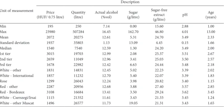
Figure 1 provides a graphical representation of the parameter estimates in the model. Path modelling groups subregions into blocks according to the wine region they belong to and then examines the paths and links between these wine regions and links between regions and wine composition, colour and varietal and individual brands in terms of regression coefficients. The model is explora- tory in nature and the algorithm is iterative, hence it is able to identify irrelevant connections. Ovals represent the LVs (blocks), and squares stand for the MVs. All the links (arrows) are significant at the 5% level, whereas the dotted lines represent non-significant links.

Based on the result of the bootstrap analysis, the regression coefficients between the LVs were proved valid. In order to verify that the SE of the regression coefficients will always be provided. Regarding the goodness of fit, the GOF of the inner model was 0.770, the GOF value of the outer model was 0.958 and the entire model has a GOF of 0.738, which shows an excellent fit.

The two main regressions of the model are Wine composition (R²=0.561) regressed by the wine regions and Colour and Varietal as well as Market Situation (Price, Quantity) (R²=0.386) regressed by Wine composition.

The proportion of variance explained in the two regressions is appropriate.

(6)

All manifest variables of intrinsic value are in a strong significant relation with Composition, and their effect is positive except for sugar content. That means that the more concentrated a bottle of wine is, the higher its price and the lower its quantity will be, while wines (outside of the Tokaj wine region) with higher sugar content are cheaper and produced in larger batches. This argument supports the findings of the majority of the literature [7,24]. Moreover, the analysis of Colour and Varietal composition shows that red wines significantly differ from white ones and rosés. The (positive) effects of the varietal composition is the highest for red wines of Bordeaux varieties. That means that red wines (especially of Bordeaux varieties) tend to be priced higher and sold in low quantities, while rosés are sold in large batches at significantly lower prices. This is very much in line with previous findings of the literature [1,2].

The effect of regional origins largely depends on the actual region. Felső-Magyarország and Pannon wine regions affect intrinsic value positively (B=0.175;

SE=0.014; t=12.6; p<0.001 and B=0.184; SE=0.016; t=11.7;

p<0.001, respectively), while the effect of Balaton and Duna regions is negative (B=-0.087; SE=0.015; t=-5.8;

p<0.001 and B=-0.225; SE=0.014; t=-15.9; p<0.001, respectively). This means that wines from Felső- Magyarország and Pannon regions are sold at higher prices, in smaller batch sizes and have higher intrinsic value. On the contrary, wines from Balaton and

Duna region wines have lower prices, higher quantity and lower intrinsic value (the composition contains less alcohol and more sugar). Felső-Pannon region is still significant but with a relatively smaller regression coefficient (B=0.044; SE=0.015; t=3.0; p<0.01). The regression coefficient of wine composition was B=0.621 (SE=0.016;

t=38.1; p<0.001) with regards to price and quantity. This suggests that the more alcohol and sugar-free extract content increases the price of wines and the quantity is lower. These results confirm previous studies suggesting the GI-based results are highly region-specific [31,32].

Collective or individual brands may alter the effects of regional origin, again echoing findings of previous literature on the topic [7,8]. Higher tier individual brands (Tier1 and Tier2) always positively affect intrinsic value and compensate potential negative regional effects. The effect of using a Tier1 brand is double to that of a Tier2 brand.

Meanwhile, the role of GIs is versatile; however, all of them were significant. In regions, where the regional origin is positively related to intrinsic value (Felső-Magyarország and Pannon), only half of the GIs strengthen this effect. The different classes of Eger (Eger Classicus (r=0.124), Eger Superior (r=0.398), Eger Grand Superior (r=0.326) and Eger before 2010 (r=0.458)) have a positive effect. In the case of Eger, however, the role of regulations must be highlighted – if certain practices are forbidden (e.g. sweetening, subtracting alcohol), and

Table 1. Descriptive statistics.

Unit of measurement

Description Price

(HUF/ 0.75 litre) Quantity

(litre) Actual alcohol

(%vol) Sugar

(g/litre)

Sugar-free extract

(g/litre) pH Age

(years)

Min 195 250 7.14 0.00 15.60 2.88 1.00

Max 23980 507284 16.45 162.70 46.80 4.01 13.00

Mean 2072 20275 12.61 5.31 24.70 3.49 2.33

Standard deviation 1937 35803 1.13 13.09 4.45 0.15 1.66

Median 1540 7540 12.59 1.30 24.20 3.49 2.00

1st tier 3015 19703 12.99 2.08 25.37 3.51 2.67

2nd tier 2659 11049 12.96 3.41 25.03 3.50 2.57

3rd tier 1678 22982 12.42 6.63 24.44 3.48 2.18

White - other 1831 14831 12.45 5.02 22.23 3.39 2.02

White - International 1857 11232 12.70 5.40 22.07 3.39 1.83

Rose 1299 26043 12.24 3.98 20.82 3.40 1.15

Red - other 2287 20956 12.68 3.88 27.40 3.57 2.85

Red - Bordeaux 3108 16684 13.41 3.50 29.24 3.62 3.45

White - Cserszegi/Irsai 1115 21352 11.61 3.43 21.33 3.45 1.24

White - other Muscat 1496 26577 11.73 19.05 21.31 3.43 1.65

Source: own composition.

(7)

thresholds on grape quality level are stricter, production technology has an impact as well.

On the other hand, Mátra (r=-0.627), Bükk (r=-0.181), Debrői Hárslevelű (r=-0.163) and Felső- Magyarország (r=-0.279) have a negative effect. In Pan- non region, it is only Szekszárd (r=0.421) and the two tiers of Villány (V.Classicus (r=0.168) and V.Prémium (r= 0.783), while Pannon (r=-0.097), Pécs (r=-0.198) and Tolna (r=-0.115) have a slightly negative effect. A higher negative effect can be found for Dunántúl (r=- 0.266). Both in the case of Eger and Villány, the effect of top tier categories (E.Superior and E.Grand Superior,

V.Prémium) significantly exceeds the effect of low tier categories (E.Classicus and V.Classicus). These results also strengthen the case-specific nature of GI price effects suggested by the literature [31,32].

There are two regions, where regional origin yields a negative effect: Balaton and Duna. Only 3 out of the 16 concerned GI has an impact that changes the negative coefficient of the regional origin into positive: Balaton- boglár (r=-0.035), Balatonfüred-Csopak (r=-0.131) and Zala (r=-0.193). All other GIs keep the negative effect of regional origin on intrinsic values. The highest impact is of Duna-Tisza közi (r=0.794), imported PGIs (r=0.464),

Figure 1. Path model and regression coefficient estimates from the bootstrapping. Source: own composition.

(8)

Balaton (r=0.587), Balatonmelléki (r=0.382). Also, Dunántúl (a PGI including the area of three wine regions:

Felső-Pannon, Balaton and Pannon) has an overall negative effect on intrinsic values, regardless of their regional origin. Not using a GI affects only the Pannon regional origin, moderating its positive impact (r=-0.097). Regard- ing Felső-Pannon regional origin has a negative effect in case of Mór (r=-0.371) and Etyek-Buda (r=-0.383) while Neszmély (r=0.545) has a positive effect on intrinsic values. Individual brands may compensate for the negative effects (r=0.125). The “without GI” variable did not have a significant correlation with any of the above wine regions but Balaton (B=-0.044; SE=0.021; t=-2.128; p=0.033).

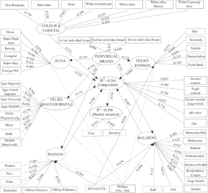
The explained deviation is presented in the main diagonal of the correlation matrix and shows how much a given LV explains from its MVs (Table 2). The figures under the main diagonal are the Pearson correlations between the LVs. The values above the main diagonal

show the significance of the Pearson correlation coefficients. It is obvious that each LV (especially the outcome Price and quantity) explains a sufficient amount of deviation of its linked items and the model does not conflict the Fornell and Larcker criterion (correlations don’t exceed standard deviations). However, in case of wine composition Colour and Varietal is also strongly correlated but not better then its MVs. Wine composition is the most correlated with Colour and Varietal, Price and Quantity and with Pannon/Duna regions.

Table 3 presents the contributions of the latent variables to Composition. Colour and Varietal explained around 62.5% of the variance in Composition, Pan- non and Duna contributed to 14.8% and 11.3% of the variance. Regarding the effect sizes it can be stated that Colour and Varietal had a large predictive ability, while Felső-Magyarország, Duna and Pannon had only a small effect on Composition.Going more into detail, the dif-

Table 2. Pearson correlations between latent variables and standard deviations.

Latent variable 1 2 3 4 5 6 7 8 9

IB (1) 0.762 <0.001 <0.001 <0.001 <0.001 <0.001 <0.001 <0.001 <0.001

CV (2) 0.081 0.414 <0.001 0.943 0.834 0.017 <0.001 <0.001 <0.001

Duna (3) 0.158 -0.099 0.397 0.943 0.834 0.017 <0.001 <0.001 <0.001

FM (4) 0.116 0.141 -0.035 0.357 0.238 0.967 0.895 <0.001 <0.001

FP (5) 0.125 0.043 -0.052 0.019 0.408 <0.001 0.082 <0.001 0.001

Balaton (6) -0.110 -0.143 0.132 -0.048 -0.286 0.284 <0.001 <0.001 <0.001

Pannon (7) 0.192 0.375 -0.127 0.047 0.191 -0.277 0.368 <0.001 <0.001

WC (8) 0.204 0.661 -0.281 0.246 0.111 -0.188 0.452 0.662 <0.001

PC(9) 0.279 0.304 -0.272 0.213 0.074 -0.087 0.390 0.621 0.764

n.r = not relevant, cannot be calculated Source: Own composition.

IB: Individual Brand; CV: Colour and Varietal; FM: Felső-Magyarország; FP: Felső-Pannon;

WC: Wine composition; PC: Price and quantity.

Table 3. Impact and contribution of the latent variables to Composition.

Description Colour & Varietal Pannon Felső-Pannon Balaton Felső-

Magyarország Duna

Correlation 0.661 0.452 0.111 -0.188 0.246 -0.281

Beta coefficient 0.531 0.184 0.044 -0.087 0.175 -0.225

VIF* 1.196 1.284 1.109 1.196 1.030 1.058

Effect sizes (f²) 0.537 0.060 0.004 0.014 0.068 0.109

Correlation x Beta coefficient 0.351 0.083 0.005 0.016 0.043 0.063

Contribution to R² (%)** 62.5 14.8 0.9 2.9 7.7 11.3

Cumulative % 62.5 77.3 78.1 81.0 88.7 100.0

(*): Variance Inflation Factor, should be lower than 3 according to Hair et al. [13].

(**): The sum of “correlation x Beta coefficient” was 0.561 and contribution to R² of a latent variable was calculated as a percentage of this value.

(9)

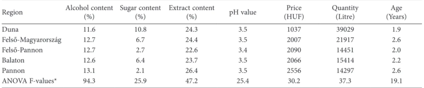
ferent wine regions show various patterns with respect to intrinsic values, price and quantity and can be clus- tered into two groups (Table 4). In the first cluster, larger batches can be observed in the case of Duna and Felső- Magyarország at lower prices. Also, these wine regions have lower alcohol content and relatively higher sugar content. Felső-Pannon, Balaton, Pannon belong to the second cluster with lower batches and higher prices and relatively higher alcohol and lower sugar content.

Pannon region is standing out with its high sugar-free extract content. F-values show significant differences among these wine regions and also highlights the most influential factors and we could determine an order. The major differences among the regions are due to actual alcohol content (F=94.3) which varies between 11.6 to 13.1 percent. The second most influential factor is sugar- free extract content followed by quantity (F=37.3) and price (F=30.2). The least significant factors are sugar content, pH value and Age but they also cause significant differences between the regions.

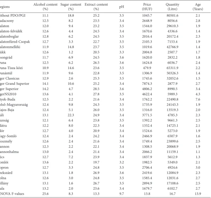
Studying the differences between the different GIs also reveal new patterns (Table 5). It is observable that wines without GIs (FN) are dominating the sample with extremely high quantity and relatively lower prices. The same holds for Duna-Tisza közi and Dunántúl. In the case of Eger wines, we can observe the lower quantities with the highest prices. Badacsony is standing out from the Balaton GIs, Kunság and Hajós-Baja from Duna GIs, Villány from the Pannon GIs and Neszmény and Etyek- Buda from the Felső-Pannon GIs regarding quantity and price. At GI level the most significant factors are also actual alcohol content, followed by quantity and price. The least influential factors are pH value and sugar content. ANOVA analysis found significant differences between GIs and region with respect to all parameters at 1% significant level. The major differences among the GIs are due to actual alcohol content (F=25.6) (this is the same at the regional level) which varies between 10.9 to

14.2 percent. The second most influential factor is quantity (F=16.7) followed by price (F=13.8). The three least significant factors are sugar content, age and pH value but they also cause significant differences between the regions.

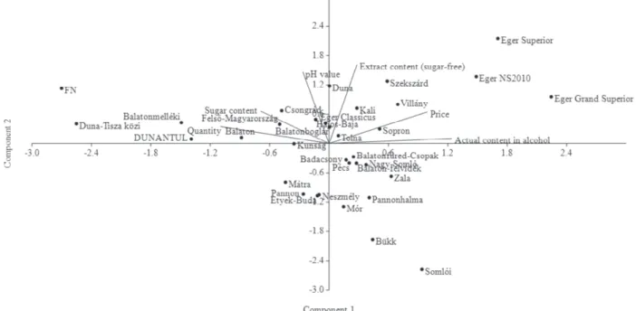
In the second step, a PCA was performed (Figure 2). The purpose of the analysis was to graphically represent the patterns of the different wine GIs with respect to the different determinants of wine prices in a two- dimensional space (biplot graph) and study the connections between the rows (subregions) and columns (determinants) of the matrix. All the PCAs were performed by using the Varimax rotation so as to create more interpretable principal components. For all the calcula- tions R 3.4.4 was used with psych package with principal and KMO function was used for calculating PCA and Kaiser-Meyer-Oldkin (KMO) tests of sampling adequacy. The total explained variance was 74% and KMO test provides 0.55 for measuring the sampling adequacy which is acceptable.

As evident from Figure 2, the first component separates explain 42% of the total variance and separates wine GIs with respect to price and actual alcohol on the right side and quantity and sugar content on the left side of the axis. Wines without GI or with GIs Duna- Tisza közi, Balatonmelléki, Balaton, Felső-Magyarország are lower priced and poor in alcohol but more sold in higher quantity and the sugar content is also higher. The opposite is true for Eger Superior, Grand Superior, Eger NS2010 and Szekszárd and Villány. The second dimension separates GIs with more relatively higher pH and sugar-free extract content like Duna, Szekszard, Eger NS2010 and Eger Superior from GIs (Somlói, Bükk, Mór, Neszmély, Pannonhalma, Pannon, Mátra) with relatively less extract content and smaller pH. The second component explained 32% of the total variance.

On the whole, we found that major differences among the GIs in terms of prices are due to actual alco-

Table 4. Regional determinants of wine prices by major wine regions.

Region Alcohol content

(%) Sugar content

(%) Extract content

(%) pH value Price

(HUF) Quantity

(Litre) Age

(Years)

Duna 11.6 10.8 24.3 3.5 1037 39029 1.9

Felső-Magyarország 12.7 6.7 24.4 3.5 2007 21917 2.6

Felső-Pannon 12.7 2.7 22.6 3.4 2090 14451 2.0

Balaton 12.6 6.4 23.7 3.5 2066 15414 2.2

Pannon 13.1 2.1 26.4 3.5 2556 14297 2.6

ANOVA F-values* 94.3 25.9 47.2 25.4 30.2 37.3 19.1

*: All the F-values are significant at 0.01 level.

Source: Own composition.

(10)

hol content and quantity, while sugar content, age and pH value had less importance. These findings also hold important lessons for policy makers. It should be under- stood that a dual wine market exists in Hungary, with producers for the two distinct segments having very different goals and ambitions. On the one hand, premium quality wines should have a higher alcohol content, have a recognisable GI behind them, and be produced in lower quantities. On the other hand, homogenous wines should be produced in large quantities and be sold at

an average price. Stakeholders in the sector should also bear in mind that it is not GI usage that matters on average but the specific GIs as we have shown above. From a consumers’ point of view, economic theories also hold – high quality wines with low prices remain supermarket slogans.

Finally, we have to mention some limitations of this study. First of all, the results are highly case (i.e. GI)- specific. Regarding the PLS approach, interpretation of the model could be harder with negative weights and

Table 5. Regional determinants of wine prices by geographical indications.

Regions Alcohol content

(%) Sugar content

(%) Extract content

(%) pH Price

(HUF) Quantity

(Litre) Age

(Years)

without PDO/PGI 11.1 18.8 25.2 3.5 1045.7 80501.6 2.1

Badacsony 12.5 8.2 23.5 3.4 2648.9 8056.6 2.8

Balaton 12.0 9.4 23.2 3.5 1544.0 29610.3 1.9

Balaton-felvidék 12.6 4.4 24.5 3.4 1670.6 4336.6 1.4

Balatonboglar 12.8 6.2 24.5 3.5 2016.4 20172.4 2.3

Balatonfüred-Csopak 12.7 3.3 22.7 3.5 2105.3 7153.4 1.9

Balatonmelléki 11.9 14.8 23.7 3.5 1019.6 42766.9 1.4

Bükk 12.6 1.2 20.5 3.3 2004.8 2507.7 1.7

Csongrád 11.7 6.9 24.5 3.6 1620.0 2832.2 1.8

Duna 12.5 6.2 26.5 3.6 1624.8 6036.7 2.4

Duna-Tisza közi 10.9 14.6 23.6 3.5 479.9 65311.9 2.2

Dunántúl 11.9 9.6 22.8 3.5 1306.9 50326.3 1.4

Eger Classicus 12.9 2.6 25.3 3.5 1745.6 32052.6 1.5

Eger Grand Superior 14.1 10.6 25.2 3.4 7874.3 2877.9 2.7

Eger Superior 14.2 4.7 28.5 3.6 4806.2 8990.5 3.4

EgerNS2010 13.6 4.1 27.8 3.5 4622.4 5989.3 4.3

Etyek-Buda 12.5 2.2 21.6 3.4 1762.2 22490.8 7.6

Felső-Magyarország 12.4 9.8 24.3 3.5 1735.9 24143.3 1.9

Hajos-Baja 12.4 5.1 26.0 3.5 1316.0 13519.3 2.0

Káli 13.1 22.3 24.9 3.4 3771.5 4785.3 2.3

Kunság 12.1 6.4 23.8 3.5 1392.2 9661.3 2.5

Mátra 12.2 8.0 22.3 3.4 1332.4 14725.1 2.1

Mór 12.7 4.0 20.9 3.4 1524.6 5273.0 1.9

Nagy-Somló 12.4 2.4 24.2 3.4 2466.9 6507.9 1.6

Neszmély 12.6 2.4 21.6 3.4 1749.4 23899.6 2.5

Pannon 12.3 2.2 22.1 3.4 1308.5 20068.9 1.9

Pannonhalma 13.0 2.4 21.4 3.4 2066.2 11159.1 1.1

Pécs 12.7 7.2 23.9 3.4 1837.9 5612.9 1.3

Somlói 13.6 2.2 19.7 3.2 1982.5 5349.0 2.1

Sopron 12.7 3.3 24.8 3.5 2706.4 4924.6 3.0

Szekszárd 13.1 1.8 26.9 3.6 2419.6 12084.9 2.3

Tolna 12.6 3.0 24.8 3.5 1585.4 12031.6 2.7

Villány 13.1 1.6 26.7 3.5 2894.9 17108.6 2.5

Zala 13.2 2.0 23.6 3.4 1679.7 6102.7 2.7

ANOVA F-values 25.6 8.3 13.3 9.7 13.8 16.7 13.9

*: All the F-values are significant at 0.01 level.

Source: Own composition.

(11)

formative measurements with negative weights could critical. There is not a global index for model validation and GOF is not advisable to use for this purpose and its use is limited. Some variables might violate the Fornell and Larcker criterion (like in our case Color and Varie- tal was strongly correlated with Wine Composition) and multicollinearity could be an issue especially in case of formative modelling.

5. CONCLUSIONS

This paper aimed to analyse the regional determinants of wine prices in Hungary by using Partial Least Squares method. The results show adverse effects on price and quantity as cheaper wines tend to be sold in larger quantities, and the opposite also holds true.

First, it becomes apparent that intrinsic values play a major but ambiguous role in regional wine prices. The higher the concentration of a compound is, the higher the price will be – with the exception of sugar. This suggests that wines with a higher concentration of alcohol and sugar-free extract and with low sugar content are made in lower quantities and are sold at higher prices.

The lower the batch size is, the easier it is to attain higher price levels. Alternatively, from the reverse perspective, we can assume that only more expensive wines are worth producing in smaller quantities (as average costs are higher in these cases).

At the other end of the market, larger batches are produced of wines with elevated sugar levels and sold at a lower price. Given the exclusion of Tokaj wines from the sample, higher sugar levels are typically a result of sweetening rather than the use of overripe grapes whose must does not ferment completely. In the case of these wines, sugar is not a sign of elevated quality level but rather a tool for creating a homogenous taste (and covering possible minor defects). Thus, the negative relationship of sugar content and price is entirely in line with theory, suggesting that homogenous wines shall be produced in large quantities and sold at an average price.

The regional dimension shows versatile effects as some regions strengthen the relationship of intrinsic values and market situation, while others weaken this effect. This is further complicated by different GIs. The results are in line with the findings of previous literature on this subject as it is not GI usage that matters, but the specific GI. The most notable GIs are Villány (V.Classicus and V.Prémium), Eger (mainly E.Superior and E.Grand Superior or older vintages) and Szekszárd.

We must note that red wines are very common with these GIs (however, whites in Eger and rosés in Villány and Szekszárd also have a significant share).

Individual brands have an essential role. Tier1 and Tier2 wineries tend to sell their wines at higher prices and in smaller batch sizes. The relationship is twice as strong in the case of the Tier1 group. On the whole, our

Figure 2. Relationship between subregions and determinants (biplot). Source: Own composition.

(12)

results support empirical literature at the country level as evident from the literature review.

Our model also suggests that wines with a low concentration of alcohol and extracts and significant levels of sugar content (i.e. semi-sweet) are sold in the lower segment of the market, characterised by fierce competition. Here, batches must be larger for the sake of effi- ciency and the concentration of chemical compounds are low for lower costs. Meanwhile, the higher end of the market shows the signs of monopolistic competition with product differentiation, higher quality level, higher prices and smaller batches.

Results also suggest that wine market policies (such as horizontal rules on GI systems) shall make the differences in quality rules more transparent for consumers. A classification of GIs by easy-to-understand quality stand- ards (based on simple indicators of grape and wine quality) may serve as a useful tool.

Moreover, the control of wine products shall be adjusted to their market situation. On the one hand, wines sold at larger quantities (and lower prices) should be controlled on the spot instead of the strict and time- consuming ex-ante control process before their release to the market. On the other hand, wines sold in low quantities and at higher prices (often using GIs or individual terms benefitting of a good reputation) should be controlled rigorously before entering to the market (including strict organoleptic tests).

Our paper can serve as a basis for future studies either by comparing our results to different regions or introducing other regional determinants (variables) to a selected region in order to give a more comprehensive picture on the topic.

ACKNOWLEDGEMENT

This article was supported by the János Bolyai research scholarship of the Hungarian Academy of Sci- ences and Supported by the ÚNKP-20-5-DE-1 New National Excellence Program of the Ministry for Inno- vation and Technology from the source of the National Research, Development and Innovation Fund.

REFERENCES

[1] G. Ferro, I.B. Amaro, What factors explain the price of top quality wines? International Journal of Wine Business Research, 30 (2018) 117–134. https://doi.org/10.1108/IJWBR-05-2017-0036

[2] L.M.K. Kwong, T. Ogwang, L. Sun, Semiparametric versus parametric hedonic wine price models: an

empirical investigation. Applied Economics Letters, 24 (2017) 897–901. https://doi.org/10.1080/135048 51.2016.1240330

[3] T. Pucci, E. Casprini, S. Rabino, L. Zanni, Place branding-exploring knowledge and positioning choices across national boundaries: The case of an Italian superbrand wine. Brit Food J. 119 (2017) 1915–1932. https://doi.org/10.1108/BFJ-11-2016- [4] E. Shane, M.D. Wahid Murad, S. Freeman, Fac-0582 tors influencing price premiums of Australian wine in the UK market. International Journal of Wine Business Research 30 (2018) 96–116. https://doi.

org/10.1108/IJWBR-02-2017-0009

[5] G. Schamel, K. Anderson, Wine Quality and Vari- etal, Regional and Winery Reputations: Hedonic Prices for Australia and New Zealand. The Eco- nomic Record 79 (2003) 357–369. https://doi.

org/10.1111/1475-4932.00109

[6] J.L. Troncoso, M. Aguirre, Short communication. Price determinants of Chilean wines in the US market: a hedonic approach. Span J Agric Res. 4 (2006), 124–129. https://doi.org/10.5424/

sjar/2006042-191

[7] P. Roma, G. Di Martino, G. Perrone, What to show on the wine labels: a hedonic analysis of price driv- ers of Sicilian wines. Appl Econ. 45 (2013), 2765–

2778. https://doi.org/10.1080/00036846.2012.67898 [8] N. Noev, Wine Quality and Regional Reputation: 3

Hedonic Analysis of the Bulgarian Wine Market.

Eastern Eur Econ. 43 (2005), 5–30. https://doi.

org/10.2753/EEE0012-8755430601

[9] K. van Ittersum, M.T.G. Meulenberg, H.C.M. van Trijp, M.J.J.M. Candel, Consumers’ Appreciation of Regional Certification Labels: A Pan-Europe- an Study. J Agr Econ. 58 (2007) 1–23. https://doi.

org/10.1111/j.1477-9552.2007.00080.x

[10] L. Barisan, M. Lucchetta, C. Bolzonella, V. Boatto, How Does Carbon Footprint Create Shared Val- ues in the Wine Industry? Empirical Evidence from Prosecco Superiore PDO’s Wine District.

Sustainability-Basel. 11 (2019) 3037. https://doi.

org/10.3390/su11113037

[11] A. Król, The Application of Partial Least Squares Method in Hedonic Modelling. Archives of Data Science, 2 (2017), 1-13. https://doi.org/10.5445/

KSP/1000058749/05

[12] X.L. Yang, Q. He, Influence of Modeling Methods for Housing Price Forecasting. Adv Mat Res. 798–

799 (2013), 885–888. https://doi.org/10.4028/www.

scientific.net/AMR.798-799.885

(13)

[13] J.F. Hair, G.T.M. Hult Jr., C. Ringle, M.A. Sarstedt, Primer on Partial Least Squares Structural Equa- tion Modeling (PLS-SEM); Sage Publications: Los Angeles, CA, USA, 2017.

[14] J. Tirole, A Theory of Collective Reputations (with applications to the persistence of corruption and to firm quality). Rev Econ Stud. 63 (1996), 1–22. https://doi.org/10.2307/2298112

[15] L. Menapace, G. Moschini, Quality certification by geographical indications, trademarks and firm reputation. Eur Rev Agric Econ. 39 (2012), 539–556.

https://doi.org/10.1093/erae/jbr053

[16] G. Anania, R. Nisticò, Public Regulation as a Sub- stitute for Trust in Quality Food Markets: What if the Trust Substitute cannot be Fully Trusted? J Inst Theor Econ. 160 (2004), 681–701. http://www.jstor.

org/stable/40752485

[17] G.C. Moschini, L. Menapace, D. Pick, Geographi- cal indications and the competitive provision of quality in agricultural markets. Am J Agr Econ.

90 (2008), 794–812. https://doi.org/10.1111/j.1467- 8276.2008.01142.x

[18] A.M. Zago, D. Pick, Labeling Policies in Food Mar- kets: Private Incentives, Public Intervention, and Welfare Effects. J Agr Resour Econ. 29 (2004), 150–

165. https://www.jstor.org/stable/40987237

[19] T. Josling, The War on Terroir: Geographical Indi- cations as a Transatlantic Trade Conflict. J Agr Econ. 57 (2006), 337–363. https://doi.org/10.1111/

j.1477-9552.2006.00075.x

[20] H.H. Ali, C. Nauges, The Pricing of Experience Goods: The Example of en primeur Wine. Am J Agr Econ. 89 (2007), 91–103. https://www.jstor.org/

stable/4123565

[21] A.M. Angulo, J.M. Gil, A. Gracia, M. Sánchez, Hedonic prices for Spanish red quality wine.

Brit Food J. 102 (2000), 481–493. https://doi.

org/10.1108/00070700010336445

[22] A.J. Blair, C. Atanasova, L. Pitt, A. Chan, A. Wall- strom, Assessing brand equity in the luxury wine market by exploiting tastemaker scores. Journal of Product & Brand Management 26 (2017), 447–452.

https://doi.org/10.1108/JPBM-06-2016-1214 [23] G. Di Vita, F. Caracciolo, L. Cembalo, E. Poma-

rici, M. D’Amico, Drinking Wine at Home:

Hedonic Analysis of Sicilian Wines Using Quan- tile Regression. American Journal of Applied Sci- ences 12 (2015), 679–688. https://doi.org/10.3844/

ajassp.2015.679.688

[24] B-H. Ling, L. Lockshin, Components of Wine Pric- es for Australian Wine: How Winery Reputation, Wine Quality, Region, Vintage, and Winery Size

Contribute to the Price of Varietal Wines. Australa- sian Marketing Journal 11 (2003), 19–32. https://

doi.org/10.1016/S1441-3582(03)70132-3

[25] R. Carew, W.J. Florkowski, The Importance of Geographic Wine Appellations: Hedonic Pricing of Burgundy Wines in the British Columbia Wine Market. Can J Agr Econ. 58 (2010), 93–108. https://doi.org/10.1111/j.1744-7976.2009.01160.x [26] P. Combris, S. Lecocq, M. Visser, Estimation of

a hedonic price equation for Burgundy wine.

Appl Econ. 32 (2000), 961–967. https://doi.

org/10.1080/000368400322011

[27] S. Lecocq, M. Visser, What Determines Wine Pric- es: Objective vs. Sensory Characteristics. Journal of Wine Economics 1 (2006), 42–56. https://doi.

org/10.1142/9789813232747_0023

[28] L.A. Panzone, O.M. Simões, The importance of regional and local origin in the choice of wine:

Hedonic models of Portuguese wines in Portugal.

Journal of Wine Research 20 (2009), 27–44. https://

doi.org/10.1080/09571260902978527

[29] S. Landon, C.E. Smith, Quality expectations, reputation, and price. Southern Economic Journal 64 (1998), 628–647. https://doi.org/10.2307/1060783 [30] C. Thrane, Explaining variation in wine prices:

the battle between objective and sensory attributes revisited, Appl Econ Lett. 16 (2009), 1383–1386.

https://doi.org/10.1080/13504850701466056

[31] E. Defrancesco, J. Estrella Orrego, A. Gennari, Would ‘New World’ wines benefit from protected geographical indications in international markets? The case of Argentinean Malbec. Wine Eco- nomics and Policy 1 (2012), 63–72. https://doi.

org/10.1016/j.wep.2012.08.001

[32] M.J. Estrella Orrego, E. Defrancesco, A. Gennari, The wine hedonic price models in the “Old and New World”: state of art. Revista de la Facultad de Ciencias Agrarias 44 (2012), 205–220.

[33] G. Schamel, Geography Versus Brands in a Global Wine Market. Agribusiness 22 (2006), 363–374.

https://doi.org/10.1002/agr.20091

[34] K.G. Joreskog, A general method for analysis of covariance structure. Biometrika 57 (1970), 239–

251. https://doi.org/10.2307/2334833

[35] H. Wold, Estimation of principal component and related models by iterative least squares. In:

Krishnaiah, P.R. (eds) Multivariate analysis, pp.

391–420. New York: Academic Press, 1966.

[36] H. Wold, Soft Modelling by latent variables:

The Non-Linear Iterative Partial Least Squares (NIPALS) approach. In: Gani, J. (eds) Perspec- tives in probability and statistics: Papers in honour

(14)

of M.S. Bartlett on the occasion of his sixty-fifth birthday, pp. 117–142. London: Applied Probability Trust, Academic, 1975.

[37] H. Wold, Soft modeling: the basic design and some extensions. In: Joreskog, K.G. and Wold, H.

(eds) Systems under indirect observation, Part 2.

Amsterdam: North-Holland, 1982.

[38] H. Wold, Partial least squares. In: Kotz, S. and Johnson, N.L. (eds) Encyclopedia of statistical sci- ences, pp. 581–591. New York: Wiley, 1985.

[39] W. Chin, The partial least squares approach to structural equation modeling. In: Marcoulides, G. (eds) Modern Methods for Business Research, pp. 295–

336. Mahwah/ London: Lawrence Erlbaum, 1998.

[40] M. Tenenhaus, V.E. Vinzi, Y.-M. Chatelin, C. Lau- ro, PLS path modeling. Comput Stat Data An.

48 (2005), 159–205. https://doi.org/10.1016/j.

csda.2004.03.005

[41] K.A. Bollen, Structural equations with latent variables. New York: Wiley, 1989.

[42] D. Kaplan, Structural equation modeling: foundations and extensions. Thousands Oaks, California:

Sage, 2000.

[43] W.W. Chin, P.R. Newsted, Structural equation modeling analysis with small samples using partial least squares. In: Hoyle, R.H. (eds) Statistical strat- egies for small sample research, pp. 307–341. Thou- sand Oaks: Sage, 1999.

[44] P.H. Garthwaite, An interpretation of partial least squares. J Am Stat Assoc. 89 (1994), 122–127. https://doi.org/10.2307/2291207

[45] D. Barclay, R. Thompson, C. Higgins, The partial least squares (PLS) approach to causal modeling:

Personal computer adoption and use as an illustration. Technology Studies 2 (1995), 285–309.

[46] S. Amato, V. Esposito Vinzi, M. Tenenhaus, A global goodness-of-8t index for PLS structural equation modeling. Oral Communication to PLS Club, HEC School of Management, France, March 24, 2004.

[47] A. Diamantopoulos, H. Winklhofer, Index construction with formative indicators: An alternative to scale development. J Marketing Res.

38 (2001), 269–277. https://doi.org/10.1509/

jmkr.38.2.269.18845

[48] J.F. Hair Jr, M.C. Howard, C. Nitzl, Assessing measurement model quality in PLS-SEM using confirmatory composite analysis. J Bus Res. 109 (2020), 101-110. https://doi.org/10.1016/j.jbus- res.2019.11.069

[49] A. Diamantopoulos, Viewpoint - Export performance measurement: reflective versus formative

indicators. Int Market Rev. 16 (1999), 444–457. https://doi.org/10.1108/02651339910300422

[50] H. Ravand, P. Baghaei, Partial Least Squares Struc- tural Equation Modeling with R. Practical Assess- ment, Research & Evaluation 21 (2016) 1-16. https://doi.org/10.7275/d2fa-qv48

[51] V. Esposito Vinzi, L. Trinchera, S. Amato, PLS path modeling: from foundations to recent developments and open issues for model assessment and improvement. In: V. Esposito Vinzi, W.W. Chin, J.

Henseler, H. Wang (eds) Handbook of partial least squares: concepts, methods and applications, pp 47–82. Springer, Heidelberg, Germany, 2010.

[52] M. Wetzels, G. Odekerken-Schröder, C. Van Oppen, Using PLS Path Modeling for Assessing Hierarchical Construct Models: Guidelines and Empirical Illustration. MIS Quarterly 33 (2009), 177–195. https://doi.org/10.2307/20650284

[53] C. Fornell, David F. Larcker, Evaluating Structural Equation Models with Unobservable Variables and Measurement Error, J Marketing Res. 18 (1981), 39–50. https://doi.org/10.2307/3151312