Behaviour Study of a Multi-Agent Mobile Robot System during Potential Field Building

Behaviour Study of a Multi-Agent Mobile Robot System during Potential Field Building

István Nagy

Institute of Mechatronics and Vehicle Techniques

Bánki Donát Faculty of Mechanical and Safety Engineering Budapest Tech

Népszínház u. 8, 1081 Budapest, Hungary nagy.istvan@bgk.bmf.hu

Abstract: In this paper a multi-agent based mobile robot simulation system will be presented where the behaviour of the system is studied with different number of agents (1, 3,6) and also with different number of ultrasonic range sensors on agents (8 or 16 US sensors on individual agents). The task of the autonomous agents is to create the potential field (PF) of an unknown environment. The classic problems of PF building, like oscillation and trapping, are not the focus of the article, but instead, the article is concerned with the agents’ self-organizing ability where self-organizing is controlled by a genetic algorithm (GA). The GA is equipped with two fitness functions where one “maintains” the distances between certain agents (spat distr), while another “watches” the area coverage (area cover). In fact, the paper can be divided into three main parts. The first part describes the ultrasonic sensing and range measuring with systematic errors, the potential field (PF) building and the moving strategies. The second part contains description of the GA, the operation of the GA, the structure of the system, the fitness functions and a general system- error determination. In the final third part, the obtained results are analyzed and presented in the appendices.

Keywords: Genetic algorithm (GA), Mobile Robot, Multi-agent, Potential Field

1 Aims and Motivation

Nowadays, in mobile robot research a huge amount of literature is available about path planning and course controlling based on a potential field. These articles are mostly about eliminating or preventing the classic problems arising in potential field building, such as trapping and oscillation. With the evolution of this area of knowledge, newer and newer methods are appearing for handling these mentioned problems, but these methods usually concern single agents. A good example can

be seen in [1], where the authors are eliminating the oscillation problem by a VFB¹ guiding model, in which at path planning the VFB is realized by a neuro- fuzzy model producing an oscillation free path between the starting and docking positions. The developed algorithm was tested in a virtual training environment named “COSMOS”, and the results can be found in the mentioned article. In relation to this, another example can be mentioned where the classic parking problem is realized by a hybrid navigation structure, with the elements of computational intelligence [2]. The hybrid structure has three components:

harmonic PF (calculation of the path in an initial – static – environment); neural network (trying to control the robot to pass through the orientation marks that the path is composed of); fuzzy controller (obstacle avoidance and trying to find the next orientation marks again). For simulation results see [2].

My primary aim is to create a functional simulation system that will be able to create the potential field of an unknown environment on a multi-agent platform.

While developing it I will not devote to the classic problems of potential field building (trapping, oscillation), but I rather wish to control the group behaviour of agents, believing that the previously mentioned basic problems can also be eliminated by this. My secondary aim is, in case of a successful system, to accomplish its analysis (see conclusion) and (probably in another article) to increase the efficiency of the algorithm by tuning the system or the GA parameters. Later in the future I would like to apply this algorithm for multi-agent systems with different sensors (e.g. visual sensors) as well.

2 Introduction

This paper actually is a continuation of the conference paper [3], and this is why the basic definitions and determinations published previously are mentioned here only in a shortened form.

Distributed problem solving at multi-agent mobile robot systems has its origin in the late 1980s [4], [5], however, since 2000, the field of cooperative mobile agents has shown dramatic development. It is reasonable to ask: Why should we use multi-agent mobile robot systems? Answering it, let me compare several advantages of multi-agent systems, as contrasted with single-agent ones.

¾ More efficiency (faster and more accurate).

Keeping to the main topic of the paper, in multi-agent systems – by exchanging the main information between one another –, the individual agents are capable to localize themselves faster and more accurately.

1Vector Field Based guiding model

¾ More fault-tolerant.

Namely, if in a single-agent system the agent breaks down, the task will not be executed, while in a multi-agent system, though depending on its intelligence, the execution of the task is continued.

Generally speaking, a multi-robot system has the following remarkable properties:

¾ Larger range of task domains (flexibility)

¾ Fault-tolerance

¾ Greater efficiency, robustness

In the development of multi robot systems, primary merits can be attributed to M.

J. Mataric (MIT, USA) whose scientific achievements include researching and developing strategies of behaviour-based mobile robot systems [6], [7], [8]. Each of these studies contains relevant statements and definitions in the field of individual or group behaviour of mobile robots. The individual agent is very well defined by Tecuci in [9] –“the agent is an autonomously active entity with certain possibilities to sense its environment and act in it in order to achieve certain states of this environment in which certain previously specified goals are achieved”.

Later, by the development of this field of science different types of agents were defined, and this can be observed very well in [10], where the basic classification of agents is extended and apart from this the agents are classified from a functional-computational perspective. After the definition of single agents, we can now focus on multi-agent systems and mainly on the cooperation between individual agents. In [11], the authors try to draw the agents into an agent coalition for the sake of a more efficient task execution. Firstly, the agent coalition is formed, the individual agents are rated and some value is assigned to them. Then, based on the agent’s value, the agent will join the coalition if the coalition brings to the agent at least the same or better results than when it works independently.

Another important contribution has been made by Fukuda and Iritani, who tried to widen the possibilities of the cooperation between separated agents in multi agent mobile robot systems [12].

The simulation system, described in this paper has a modular structure. There is a separate module for the sensory system of the agents (which is the mathematical model of the ultrasonic range detector), another module contains the GA, responsible for near-optimal behaviour selection, and the next separated module is responsible for displaying results and assessments.

Since the simulation system has been prepared in a MATLAB environment, it is inevitable to make the mathematical model of the system. The workspace is digitally decomposed (grid construction), and the agents are point-represented in this model. The visited areas are renumbered during the process of map-building, in order to avoid duplicity of the map occurring in the same area. The potential field building and calculation is based on the principle of the well-known

repulsive forces. A simplified map building process by one agent is represented on Figure 1. The agent moves to the new position, assigns the position to the grid construction of the model, performs distance measurements, evaluates the potential field value (broadcasting the parameters of its own new position to the other agents), and then plans the next move. The potential field values are stored on the host remote server, where the global potential field map of the whole WS will be updated. In the advanced systems (will be represented in this paper), in order to avoid collisions, the moving mechanism is controlled by the GA.

Move to

P0 (x0,y0) Take N measurements [D1,..Dn]

Association to the grid Pj (xj,yj)

Update the map (based on evaluated values)

Planning the next motion

Figure 1

A simple map building process

3 Sensing

The individual agents are equipped with 8 or 16 ultrasonic sensors for distance measurements. The sensors are equally spaced on a ring around the body of the robot (see Figure 2a) so that the sensors form a regular octagon (or a polygon with 16 points) on the circle of the agent. In this case the sensing sector of each sensor can be calculated with the form:

2 ; N

β = π

(1)

where, N is the number of sensors. The sensors can also choose either long- or short-range sensing. The long-range sensing (LRS) perceives the obstacle or other agents in the given sector (β) in infinite² distances. The short-range sensing (SRS) is determined in a circle with radius R0. Occupation of the segments by other agents or obstacles, is represented with a binary word, and will have importance in choosing the next behavior or the moving mechanism.

β

Figure 2a

The agent, and the sensors around, located by angle β

2infinite=beyond the given radius R0

R0

MSB B1

B2

B6

Figure 2b

The Long, and Short range sensing

Let us see the illustration given on Figure 2b, where the binary words of short- respectively long-range sensing are:

LRS: 00101010 SRS: 00000011 Mathematically can be written:

, ; 0

, 1

⎪⎩

⎪ ⎨

⎧

∉

∀

∈

= ∃

j i

j i

j

P

b P

ε

ε

(2)

where, bj is the value, given by the j^th sensor, and Pi is the position of i^th agent in sector εj. In case of short-range sensing the sensing sector (εj) is valid only in the given R0 radius.

};

|

|

|

{ P

_i

P

_i

P

₀

R

₀

j

= − <

ε

(3)

where, Pi is the position of i^th agent, and P0 is the position of reference agent [13].

The surrounding environment of the reference robot is represented with the binary words LRS and SRS. We can say that two binary words are equivalent if the number of 1s and the position of 1s in relation to one another are identical (e. g.

the words ς1=01100000 és ς2=00000110 are equivalent). It is observable that with shifting to left or right, or with circular operations we can get several equivalent words. Let us name these equivalent bits stimulus and label (ς). The stimulus contains the description of the environment of the mobile robot [13].

In the perception model, the starting positions of the agents are already known (see Appendix 3). In an ideal case, the (d) distance is calculated from the time of

flight (t) and the spreading of speed of sound (v), in case of ultrasonic range measurements [14].

; 2 . 1 v t

d =

(4)

In this model the ideal case is considered, that is after checking the sensing segment’s occupation, the distance calculations in x and y directions has been provided. The distance measurement model can be seen on Figure 3.

Error

P0

Pj

Di0

j

D~i

j

Dˆi

ρj

The edge of the sensed object

β

γ

Figure 3

The mathematical model of US sensing

As a result of WS rasterizing (grid construction), an exact result of distance measurement is almost impossible. Unfortunately this is inconceivable in real environment, since we have to take into consideration the error (δ_D), see Figure 3.

ˆ |;

| ~

_i^j _i^j

D

= D − D

δ

(5)

where, D~_i^j

is the real distance, and Dˆ_i^jis the evaluated one.

);

16 ..

1 ( . , 8 ..

1 , cos

ˆ D⁰ . i resp

D_i^j = _i −ρ_j β = (6)

The distances measured with N ultrasonic sensors are stored in the L measuring- vector. The measuring-vector belonging to the P0 location is: L0≅[D₁⁰,D20,..,D80].

Besides, the evaluated distances in the model (after the grid association) belonging to the Pj position are stored in the distance-vector: ˆ [ˆ , ˆ ,.., ˆ ]

8 2

1j j j

j D D D

L = . The

errors depend on the complexity of the environment and certainly on the map grid

width (see Figure 3). With reference to the members of Lj vector, for the sake of better evaluation results, the weighting vector (wi) has been introduced. Regarding the distance between the robot location and Pj raster position, the weighting can be written as:

2; e j

w_j = ^−ηρ (7)

where η is a positive constant, and ρ_j is the distance between P0-Pj locations (See Figure 3). Namely wj=1 if the agent is exactly in the position Pj (in this case Pj≡P₀).

4 The Potential Field

The creation of the artificial potential field (APF) has been done by the well- known repulsive force method [1], [13].

)];

( [

; 0

;

; 1) (1 2 1 ) (

) 2 (

) 1 (

) ( ) ( )

(

0

0 2

0 2

x U F

l x if

l x l if

x x U

x x k x U

x U x U x U

ART ART

OBS

GOAL p

GOAL

OBS GOAL

ART

−∇

=

⎪⎩

⎪⎨

⎧

>

≤

= −

−

−

=

+

=

G

η

(8)

where, UART is the APF, UGOAL is the potential field spreading from the goal, UOBS

is the potential field of the obstacle, kp is a positive gain, l0 is a threshold limit beyond which are no repulsive forces, and η is a positive constant.

The potential field building

In case of validity of the next condition:

; ˆ 0 ], , 1

[ ≥

∈

∀i N Di^j (9)

the potential field is calculated from the Lˆ vector. This condition is valid for the _j visibility of Pj position simultaneously. If the above mentioned condition is not valid, it means that the agent is on the obstacle, or is part of the obstacle. The evaluated value of the potential field at the location Pj in step “t” (if the above mentioned condition is valid), is:

ˆ ;

1

∑

ˆ

=

≅ ^N − i

D t

j

j

e i

U ^λ (10)

where λ is a positive coefficient. The potential field values, belonging to Pj

position, measured by k^th mobile robot, at time “t”, are stored in set Ω.

ˆ };

ˆ ,.., ˆ ,

{

^t_j^{1 t}_j^{2 tk}_j

t

j

= U U U

Ω

(11)

In case if a member of Ω^t_j set equals zero, then is valid:

⎪⎩

⎪⎨

⎧ −

= Θ

Θ

∪ Ω

=

Ω ⁻

; ,

0

);

9 ˆ (

ˆ ,

1 ;

otherwise

valid is L for if U^tk_{j j}

t j t

j

(12)

To the Ω^t_j set, is associated the following confidence weight vector:

};

,.., ,

{ ^t_j^{1 t}_j^{2 tk}_j

t

j w w w

W = (13)

where the normalized weight component of W_j^tis:

;

∑

=1

− = _k

n tn j ti ti j

j w

w w (14)

Finally an acceptable potential field value can be readily calculated as follows:

⎪⎩

⎪⎨

⎧ ∃ ∈ =

=

∑

=

− ; ˆ . :

; 1 ], , 1 [ ˆ ,

1 k i

ti j ti j

ti j ti

t j

j else U w

w k i if

U U (15)

5 Motion Mechanism

After the execution of sensing, measurements, and estimating the value of the potential field in position P0, the agent has to move to the next position to continue its measurements. This move can be applied as based on three motion selection [13]:

Directional1 – here the standard deviation of potential field is calculated in all (N) sensing sectors within the given maximum movement step (dm) at time “t” and “t- 1”. Moreover, the move in time “t+1” will be calculated according to the motion direction (φ) and motion step (d_s). For the P0 location of the robot at time “t+1”

can be written:

;

0

.

1

0 jφ

s t

t

P d e

P

⁺

= +

(16)

Let us store the difference of the standard deviations of potential fields at the same sensing vector, at time “t” and “t-1” in vectorΔ.. Then the i^th component of this vector is:

});

,..

2 , 1 , ,

|

({l l U U ¹ j i N

std _{ij ij ij}^t _ij^t _i

i= = − ∀ ∈ =

Δ ⁻ ε (17)

Besides, let array Λ be the standard deviation of potential field for all locations in the same sensing sector at time “t”. For the i^th component of this vector can be written:

});

1

|

| , ,

|

({ = ∀ ∈ − ≤

=

Λ_i std v_ij v_ij U_ij^t j ε_v j i (18)

where ε_v is defined similarly like ε_i, - see above. After that, the motion direction in sector i:

; ,

);

,.., , max(

| _{1 2}

i j

N i

i

P

j ε

φ

∉

∀

Δ Δ Δ

=

Δ (19)

where Pj is the location, and ε_i is the sensing sector. Namely, the agent will select its direction of movement (φ) in “i” sector, based on the condition (19). The exact position,

P

₀^t+1

( x

₀

, y

₀

)

, within the selected sector, should satisfy the following condition:

,...);

, max(

) , (

| ) ,

(x₀ y₀ Λ_i x₀ y₀ = Λ₁ Λ₂ (20)

Directional2 – The strategy is almost the same as previously (see Directional1), the only difference being in selecting the exact position within the selected sector.

The exact position selection is based on the minimum value of vector Λ.

,...);

, min(

) , (

| ) ,

(x0 y0 Λi x0 y0 = Λ1 Λ2 (21)

Limited random – The agent selects its motion direction and step size randomly, within the given limits.

φi=rand([1..N]); (22)

ds=rand([1..dm]); (23)

The next question should be about how to make the potential field building process more effective. The answer lies in the appropriate behaviour mechanism.

6 Behaviour Selection Mechanism

Usually, in behaviour-based task execution at mobile robots, the next behaviour is very much influenced by the environment (as we know, the environment of the mobile robot is represented by stimuli; see above). In a general case, it exists as a set of behaviours out of which the best behaviour will be chosen by the algorithm, based on the environment’s appraised measurements.

Behaviour in single agent environment – Let the primitive behaviour correspond to the direction of the 8 (or 16) ultrasonic sensors (see Figure 2b, {B1, B2, …B8}).

In other words, the elementary motions are summarized in vector B, B=[B1..BN].

The values of this vector can be Bi∈{-1,1} in such a way that: Bi=1, if the agent is capable of executing the required move, else Bi=-1. The behaviour and the weighting vectors are:

; . .

2 1

⎥⎥

⎥⎥

⎥⎥

⎦

⎤

⎢⎢

⎢⎢

⎢⎢

⎣

⎡

= BN

B B

B ;

. .

2 1

⎥⎥

⎥⎥

⎥⎥

⎦

⎤

⎢⎢

⎢⎢

⎢⎢

⎣

⎡

= wN

w w

W (24)

where, the values of weighting: Wi=-1, if Bi=-1, and in other cases the weighting is:

; 1

| ₁

1

− =

= ≠

∑

wi

N

i Wi ⁽²⁵⁾

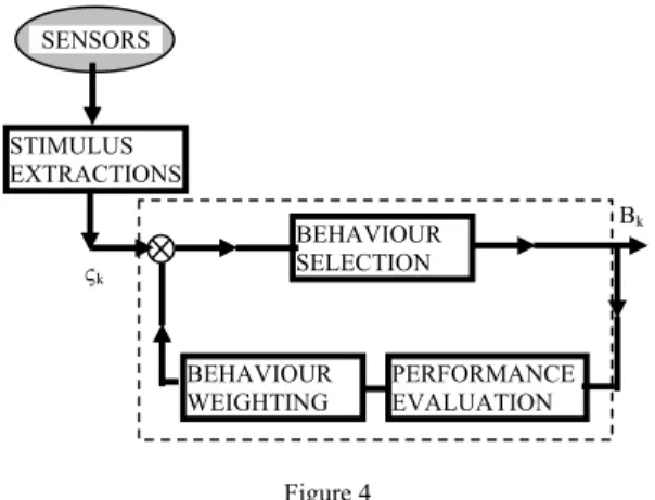
The simplified behaviour selection process can be summed up as follows: Based on the sensing vector (see LRS, SRS mentioned above), the appropriate stimulus is given which triggers a condition for the behaviour selection mechanism. Next, as the output of the embedded learning mechanism (See Figure 4; dashed line), the near optimal behaviour will be selected. Let us have a few more words about the simplified learning mechanism. Any response to the sensing vector of the agent (what is nothing else than a stimulus, and the response to the stimulus, which is the behaviour) is represented by the varying weight. The learning step is the following: if the agent has selected the motion direction, then the components of the W vector will be updated. As a result of a series of updating, the outcome will be some more significant directions.

STIMULUS EXTRACTIONS

BEHAVIOUR SELECTION

BEHAVIOUR

WEIGHTING PERFORMANCE

EVALUATION ςk

Bk

SENSORS

Figure 4

The simplified behaviour selection

The process: a stimulus (ς_k) is chosen, to which the appropriate behaviour (Bk) belongs, next the motion is executed, and then the operation is appraised by weighting (W). The next stimulus-behaviour pair selection is based on this weighting vector, which produces a more effective motion mechanism.

Behaviour in a multi-agent environment – Let the agent to the stimulus (ς_k) select the behaviour (Bk), at time „t”. After it, the robot learns, based on its local performance criteria. In the case if a common basis for behaviour selection is used, the agents can share their learned knowledge. The behaviour weight vector will be updated, based on the following:

));

(

1 normal(shapeW W

W_ς^t_k⁺ = _ς^t_k +Δ (26)

where operator “normal” is normalizing the weight vector, and ΔW is an increment vector. The performance of operator “shape” is illustrated on Figure 5, where the updated weight vector passes through function1, and conditionally function2 [15].

Function_1 Function_2 Wi+ΔWi

W0

Figure 5 The “shape” operator

The function1:

; 1 ,

1

1 0

,

0 ,

0

0 ⎪

⎩

⎪⎨

⎧

>

≤

≤

<

=

i i i

i

w if

w if w

w if

w ⁽²⁷⁾

The function2:

1 ;

0 α ₋ψ

= + ₋

wi

w e (28)

where coefficients α and ψ influence the shape of the function. Then, the j^th component of the ΔW weight-increment vector is:

, ; 0

,

| _{( )}

⎩⎨

⎧

≠

= =

Δ if j k

k j w_j

δ

^{E Bk} if

(29) where E(Bk) is an evaluation of behaviour Bk and δ∈[-1,1]. At time t=0, the i^th

component of the behaviour weight vector is:

, ; 1

1 ,

1

0

⎪⎩

⎪⎨

⎧− =−

= otherwise B if w

i i

β

(30)

where β is the number of the feasible behaviours.

Behaviour selection mechanism – this mechanism assigns the behaviour weight to the corresponding behaviour (sel: W→Bk.). The behaviour selection mechanism can work in two ways:

a) selection based on the probability of the behaviour weight vector distribution:

;

|

_{( )}

wk

P k

k

B

B

_ς

=

(31)

b) selection based on maximum weight:

;

|

_{max( , ,.. )}

2

1 N

k w w w

w k

k

B

B

_ς

=

₌ (32)

After behaviour selection the agent moves along in the selected direction, with step size d0. Let us mark the position at time “t”→P^t, and at time “t+1”→P^t+1. In this case this whole process (action) can be defined as [15]:

);

, ,

( ₀

1 t

i k t

i action B d P

P⁺ = (33)

The next step in behaviour based robotics was, mainly in environments where multi-agent robot groups occur, that for the selecting of near optimal behaviour genetic algorithms and/or neural networks were used. In this paper the near optimal behaviour is selected through a genetic algorithm which is working with two fitness functions. The essence of behaviour-control is that the agents are organized into robot groups, the efficiency of the individual agents is evaluated, and then based on this evaluation the next “action” is selected. In “action”, the direction selection is considered with two situations. The first is the spatial distribution of agents (when the distance between two agents i and j is less than

the given threshold distance: dij≤R2). The second is the area coverage, when dij>R2.

Spatial distribution - For the reference robot i, and m – neighbouring robots, is valid:

; ,

], , 1 [

, m M m i d R₂

i ∀ ∈ ≠ _im≤

; _¹

1

i j i im m j

m

d e distre

spat ^{d m θ}

γ ≅ξ

− −

=

(34) Area coverage:

; ,

], , 1 [

, m M m i d R₂

i ∀ ∈ ≠ _im>

i j i n N n j N

n

D e ere

area ^θ

π

ξ

= 0 ≅

2

1

cov

_ (35)

where, dim is the distance between robot i and m, then md is the number of group robots inside of R2 threshold limit, γ_m is the relative angle of motion direction (see Figure 3, where m^th agent is moving to Pj location and θ_i≡ρ_i), and

D

_n⁰is the n^th component of L0 vector.

Let the significant proximity direction a time t be

θ

_i^u (that is the direction of the i^th agent’s motion is u, where u is one of the 8/16 sensing sectors: u∈[1..N]).

There exists a probability vector ϖ_i, where the components express the efficiency of (34) and/or (35) if the motion was executed. This ϖ_i vector can be written as follows:

ϖi=[φ1, φ2, … ,φN];

where φ_k∈[0,1] and

∑

^N_k=₁φ_k =1;. In case if the agent in the next motion (at time t+1) selects a different motion direction “v”, (v∈[1..N]), denotes it by

θ

_i^v, then the k^th component of the ϖi vector will be updated as follows:

0 ;

1 ,

1 ;

1

⎩⎨

⎧ = − +

= +

= +

+

otherwise u v k if where

t t k k

δ ψ

ψ δ φ φ

(37)

where ψ is a positive coefficient. As a result of permanent updating some motion directions become more significant than others.

7 Genetic Algorithm

In this system the near optimal motion direction is selected through a GA. The simplified operation of the genetic algorithm works as follows:

ƒ The fitness of each member in a GA population is calculated according to an evaluation function (fitness functions), which measures how well the individual performs.

ƒ Individuals performing well are propagated in proportion to their fitness; on the other hand, the poorly performing members are reduced or eliminated completely.

ƒ By exchanging the information between members it is possible to create new search points, by which the population explores the search space and converges in an optimal solution.

To find and represent these new search points, the GA uses its operators. Several operators are known, but the three most frequently used ones are: reproduction (selects the fittest members and copies them exactly; crossover (swapping some part of their representations.); mutation (prevents the loss of information that occurs as the population converges on the fittest individuals).

In every step the mobile robot checks its environment, then according to the vectors (34), (35) and the probability vector ϖi, (what is the result of the learning process), next motion direction is selected. In compliance with this probability vector, the GA population will be determined on the basis of this ϖ_i vector. The structure of this whole system can be seen on Figure. 6.

Unknown Environment

local Stimulus

Local- map updating

World map Building

Criterion_1 Spatial diffusion Criterion_2 Area coverage

Strategy Selection

New spatial configuration

Stimulus- response Pairs Global

feedback

Stimulus response pairs DB updating

Behavioural Vector-based Experience Sharing

Action Sensing

Figure 6

The architecture of the system

Inside the dashed lines the GA module can be seen. For chromosome representation let us define a 2D coordinate frame, centred at the current location of the agent, and square bounded, where the sides are determined by the maximal step size (2.dm+1). In accordance with this, the local region for the agent’s next movement is: x’, y’∈[-dm, dm]. Moreover, let us suppose that (2.dm+1) corresponds to a binary string L, following from the fact that location within the local region can be represented by two binary values, with length L. For the behaviour evolution of a single agent, we can use a chromosome of length 2L, and for a group with M robots it is 2LM.

The fitness functions – In this system 3 fitness functions are used, out of which the 1^st is the general fitness function (fg), used for exploring less confident regions and for avoiding the repetition of other agents’ work [13].

}

; })

max{

1 (

1 1

4 1

∏ ∏

= ⎩⎨⎧ =

−

−

= ^m

i

m

j ij tk

i g

e

R d w

f (38)

where

w

_i^tk is the confidence weight corresponding to the location of agent i, then m is the number of agents grouped together during one evolutionary movement step, me is the number of robots which do not belong to m, that is the inter- distance between two robots i and j is greater than R1 (dij>R1). The 2^nd and 3^rd fitness functions are special functions, and correspond to the criteria of multi- robot spatial diffusion and area coverage, see relations (34), (35).

;

;

1 2

1

1 1 2

1

∏

∏ ∏

=

−

= =+

= Δ

−

=

c

d d

m i

i m

i m

i

j ij

f

R d f

ξ

ν (39)

where, md is the number of robots with inter-distances dij>R2, where mc is the number of area-covering robots, Δν is the number of location visited by agents m_c and ξi is the proximity distance between robot i and other agents. The complete fitness function can be defined as follows:

robots ; covering area

for , .

robots diffusing spatially

for , .

2 1

⎪⎩

⎪⎨

⎧

= − f f

f F f

g

g (40)

8 The System Error

At simulation systems the question of system errors is not avoidable. There are several possibilities to error definition. Usually at models related to mobile robots, we can define errors arising from: a) non-ideal mathematical models, b) discretization of the work space. Of course each of these errors is repairable. The 1^st is repairable by the more exact mathematical models, and the 2^nd one by scaling. In the present system, the error arising from discretization of the WS is formally defined as follows [13]:

; ˆ ) (~ 1

1

∑

2

=

−

≅ ^K

j

j t

j U

K U

εt (41)

where K, denotes the total number of locations in the potential field map, and

j t j U

U~ , ˆ belongs to the estimated and true potential field values at position Pj(xj,yj).

Conclusion

It is a simulation system for potential field building process in the multi-agent domain that has been described in this paper. The aim is to provide an opportunity for studying the behaviour vectors of agents, for the sake of selecting the near- optimal behaviour.

The aims stated in the first section (aims & motivation) have been fulfilled. A working multi-agent based simulation model has been created and the features mentioned in the second section (introduction), namely “more efficiency”, have

“more or less” been realised as well. Let us look at one of the most important elements of the list: “faster and more accurate”. An unambiguous answer is given in Appendix 5, where on Figure 12 it is clearly seen that in case of a single agent, the system was not able to create the potential field in 30 steps, while in case of 3 or 6 agents (Figures 13 and 14) it was accomplished successfully. Another conception of mine was that the basic problems of trapping and oscillation will be solved by a GA algorithm. The idea has proved to be successful too, as seen in the 5^th interval on Figure 15b in Appendix 6, where in case of single agent the problem is clearly visible, while on Figures 16 and 17 (in case of 3 or 6 agents) this problem is not present. The reason why I used the words “more or less” above is because I expected slightly better results from the aspect of area coverage. In my view, in case of 6 agents it is possible to improve the area coverage by tuning the GA parameters and fitness functions.

Appendices

This paper contains 6 appendices. In Appendix 1 the geometrical 2D map of the WS and its exact potential field can be seen. Appendix 2 includes tables with system parameters, GA parameters and computer parameters, used in the simulation. In Appendix 3 the starting positions of mobile agents can be found, while Appendix 4 contains the table and graph of running times with different number of agents and sensors. In Appendix 5 the resulting PFs are seen, also built up by different number of agents and sensors on the agents, while in Appendix 6 the wandered trajectories are represented in 6 intervals.

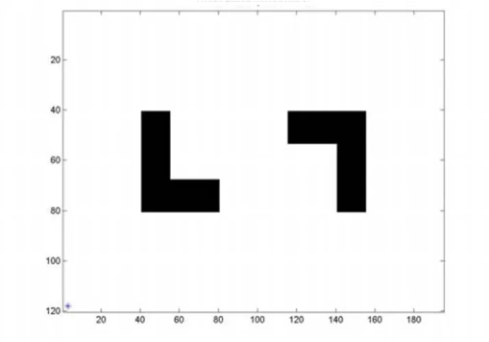
Appendix 1

The Workspace and its exact potential field

Figure 7

The WS in 2D with two obstacles

Figure 8 The exact PF of WS

Appendix 2

Tables of parameters used in the system and in the GA

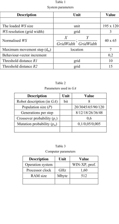
Table 1 System parameters

Description Unit Value

The loaded WS size unit 195 x 120

WS resolution (grid width) grid 3

Normalised WS

GridWidth Y GridWidth

X ; 40 x 65

Maximum movement step (dm) location 7

Behaviour-vector increment 0,2

Threshold distance R1 grid 10

Threshold distance R2 grid 15

Table 2 Parameters used in GA

Description Unit Value Robot description (in GA) bit 8

Population size (P) 20/3045/65/90/120 Generations per step 8/12/18/26/36/48 Crossover probability (pc) 0,6

Mutation probability (pm) 0,1/0,05/0,005

Table 3 Computer parameters

Description Unit Value Operation system WIN-XP, prof.

Processor clock GHz 1,60 RAM size Mbyte 512

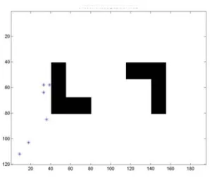
Appendix 3

The starting positions of the mobile robots

Figure 9 Starting position of 1 agent

Figure 10 Starting positions of 3 agents

Figure 11 Starting positions of 6 agents

Appendix 4 Table of results

Table 4 The Running Times

Running Times (in seconds)

Maximum number of steps 5 30 Number of sensors 8 16 8 16 Number of robots ↓

1 37 31 208 195

3 77 150 595 657

6 177 240 1162 1521

Graph-1: The running Times

0 500 1000 1500 2000

1 robot 3 robots 6 robots

Num ber of Robots

Running Time [sec]

X robot(s), 5 steps, 8 sensors

X robot(s), 5 steps, 16 sensors

X robot(s), 30 steps, 8 sensors

X robot(s), 30 steps, 16 sensors

6 robots 30 steps 16 sensors

Appendix 5

a.) b.)

Figure 12

The resulting PF of WS, built up by 1 agent in 30 steps a) 8 sensors, b) 16 sensors

Figure 13

The resulting PF of WS, built up by 3 agents in 30 steps:

a) 8 sensors, b) 16 sensors

a.) b.)

Appendix 6

Figure 15a

Trajectories of 1 agent, in 6 intervals, MaxRunStep=30, 8 sensors Figure 14

The resulting PF of WS built up with 6 agents in 30 steps:

a) 8 sensors, b) 16 sensors

a.) b.)

Figure 15b

Trajectories of 1 agent, in 6 intervals, MaxRunStep=30, 16 sensors

Figure 16a

Trajectories of 3 agents, in 6 intervals, MaxRunStep=30, 8 sensors

Figure 16b

Trajectories of 3 agents, in 6 intervals, MaxRunStep=30, 16 sensors

Figure 17a

Trajectories of 6 agents, in 6 intervals, MaxRunStep=30, 8 sensors

Figure 17b

Trajectories of 6 agents, in 6 intervals, MaxRunStep=30, 16 sensors

References

[1] S. Mizik, P. Baranyi, P. Korondi, M. Sugiyama: Virtual Training of Vector Function-based Guiding Styles; Transactions on Automatic Control and Computer Science, ISSN 1224/600X Vol. 46(60) No. 1, pp. 81-86. 2001 [2] J. Vaščák: Navigation of Mobile Robots Using Potential Fields and

Computational Intelligence Means; Acta Polytechnica Hungarica, ISSN 1785-8860, Vol. 4, No. 1, pp. 63-74, 2007

[3] I. Nagy, A. L. Bencsik: A Simulation System for Behaviour-based Potential Field Building in Multi-Agent Mobile Robot System; Proc. of the 3^rd IAESTED International Conference on Computational Intelligence, pp. 7- 12, ISBN: 978-0-88986-672-0, Canada, 2007

[4] T. Fukuda, S. Nakagawa: A Dynamically Reconfigurable Robotic System;

In Proc. of the International Conference on Industrial Electronics, Control and Instrumentation, pp. 588-595, Cambridge, MA, 1987

[5] H. Asama, A. Matsumoto, Y. Ishida: Design of an Autonomous and Distributed Robot System: ACTRESS; In proc. of the IEEE/RSJ, International Workshop on Intelligent Robots and Systems, pp. 283-290, Tsukuba, 1989

[6] D. Goldberg, M. J.Mataric: Coordinating Mobile Robot Group Behaviour Using a Model of Interaction Dynamics; Proc. of the 3^rd Int. Conf. on Autonomous Agents, pp. 100-107, Seattle, 1999

[7] P. Pirjanian, M. J.Mataric: Multi-Robot Target Acquisition Using Multiple Objective Behaviour Coordination; In proc. of the IEEE International Conference on Robotics and Automation, San Francisco, 2000

[8] M. J. Mataric: Behaviour-based Robotics as a Tool for Synthesis of Artificial Behaviour and Analysis of Natural Behaviour; Trends in Cognitive Science, 2(3), pp. 82-87, 1998

[9] Gh. Tecuci: Building Intelligent Agents; Academic Press, San Diego, Cal., 1998

[10] J. Kelemen: Agents from Functional-Computational Perspective; Acta Polytechnica Hungarica, ISSN 1785-8860, Vol. 3, No. 4, pp. 37-54, 2006 [11] B. Frankovič, T-T. Dang, I. Budinská: Agents’ Coalitions Based on a

Dynamic Programming Approach; Acta Polytechnica Hungarica, ISSN 1785-8860, Vol. 5, No. 2, pp. 5-21, 2008

[12] T. Fukuda, G. Iritani: Construction Mechanism of Group Behaviour with Cooperation; In Proc. of the IEEE/RSJ International Conference on Intelligent Robots and Systems, pp. 535-542, Pittsburgh, 1995

[13] J. Liu, J. Wu: Multi-Agent Robotic Systems; CRC Press LLC, ISBN 0- 8493-2288-X, 2001

[14] G. Dudek, M. Jenkin: Computational Principles of Mobile Robotics;

Cambridge University Press, ISBN 0 521 56021 7, 2000

[15] I. Nagy: Genetic Algorithms Applied for Potential Field Building in Multi- Agent Robotic System; In Proc. of the IEEE International Conference on Computational Cybernetics, ICCC 2003, pp. 105-108, Siófok, Hungary, 2003