DOI: 10.1556/066.2018.47.3.2
A NEW MODEL OF THERMODYNAMICS. EXTENSION OF CHEMICAL THERMODYNAMICS TO COMPLEX MATERIALS
OF CELLULAR STRUCTURE
F.Á. MOHOS
Institute of Food Engineering, Faculty of Engineering, University of Szeged, H-6724 Szeged, Mars tér 7. Hungary (Received: 28 June 2017; accepted: 6 March 2018)
This paper presents a structural model of complex materials that are partly or entirely of cellular structure, and a new model of thermodynamics, which can be applied to the processes taking place in complex materials. Since the complex materials always contain cellular fraction, the supposition of cellular equilibrium is real. The complex materials are characterized by polyagent behaviour. Therefore, new concepts such as principal variables, redundancy, macroscopic/microscopic uncertainty are defi ned, moreover, the application of chemical thermodynamics is limited to micro processes only, and the free energy (F) and the free enthalpy (G) function cannot be generally applied to calculations concerning the bulk amount. Temperature as only a local intensive variable can be discussed. The fi rst law of thermodynamics is expressed in the traditional way. The second law applied to the processes taking place both in open and in adiabatically closed systems is formulated as in words as an equation of stability, completed by the relations to fi rst and second differential of entropy. In connection with the second law the Damköhler balance equation system, the Rabinowitsch–Mooney equation, and the application of dimensional analysis are presented.
Only the apparent thermal capacities can be used for complex materials in general. The data of specifi c thermal capacity of complex materials in the proximity of absolute zero temperature are not suffi cient for drawing conclusions on their entropy. The concept ‘shelf-life’ is essential in food science and practice, a Monte-Carlo method is presented for its calculation.
Keywords: three laws of thermodynamics, structural model of complex materials, polyagent behaviour, macroscopic/microscopic uncertainty, redundancy, dynamical processes, shelf-life, Monte-Carlo method
1. Introduction
There are plenty of complex, animate/inanimate bodies surrounding us, which are either of cellular structure (e.g. living trees/plants/animals, etc.) or composites consisting of cellular substances and multiphase systems. The cellular substances cannot be chemically defi ned, because they are not chemicals, albeit they can be studied by using the tools of chemistry. The boundaries of chemical thermodynamics are established by Gibbs’ Phase Rule that refers to multiphase systems (MOHOS, 1982, 2010, 2017). Consequently, the degree of freedom, which is based on the Phase Rule, cannot be calculated for systems of complex materials. By studying the properties of complex materials of cellular structure as a whole, present paper enables enlarging the boundaries of chemical thermodynamics from the atomic kernel up to the organism.
2. The structural peculiarities of complex materials
2.1. Hierarchic levels of the structure of complex materials
The structure of various substances is characterised by a hierarchic nature (MOHOS, 1982, 2010, 2017). An optional classifi cation for these various levels of hierarchy can be generally defi ned as follows:
“Microsystems”:
- Atoms, activated atoms - Atomic groups, molecules
- Phases of molecules (multiphase systems)
--- (An imaginary line)
“Macrosystems”:
- Cells of tissue, fractions of cell - Tissues, fractions of tissue - Organs, fractions of organ
- Organism (animate/inanimate), fractions of organism, microbial cells
Independent of any classifi cation, it is to be emphasised that cellular materials represent a radically different quality compared to that of chemicals. (The imaginary line above tries to stress this fact.) Every cell is a peculiar “chemical factory”. At the same time, chemistry itself is limited in explaining the substantive nature of cells, it exclusively offers an explanation concerning the nature of its chemical ingredients. Thus, studying complex materials leads to facing the epistemological problem of “part and whole”:
Part → chemical properties of the cellular system
Whole → ‘global’ (chemical, physical, biological) properties of the cellular system Nevertheless, studying the single cell already points to the diffi culty of its chemical nature: the polyagent behaviour. Moving forward to “higher” hierarchic levels (tissues, organs, etc.), this polyagent behaviour becomes even more essential, and needs to be taken into consideration.
Complex materials can be studied both as microsystems (e.g. the chemical processes taking place in a certain portion of them) and as macro systems, that is the processes taking place in bulk. For example, during baking bread, plenty of chemical and physical-chemical changes (dehydration, oxidation, Maillard reaction, coagulation, etc.) are taking place in the dough, which can be studied separately as microsystems.
2.2. Polyagent behaviour – Microscopic and macroscopic uncertainty
2.2.1. Polyagent behaviour. Numerous processes are taking place simultaneously in complex materials, but their exact number cannot be precisely determined. This reveals a special feature of complex materials, namely the polyagent (or multi-agent) behaviour, meaning that simultaneously and practically at the same place many participants (chemical components, material fractures, microbae) contribute to various types of change (chemical reactions, physical, biological processes) at several hierarchic level. The qualities and quantities of these agents cannot be exactly determined in most cases, they depend on the analytical method and the equipment applied. For example, the number of natural etheric oil fractions determined in an extract basically depends on the sensitivity of analytics; and any restitution of the original extract in line with the analytical results will never result in the original
Gibbs region
properties. This example also shows that our understanding of the original properties will always be limited. As an essential feature of complex materials, the uncertainty in relation to the number of chemical participants is always actual because of the polyagent behaviour.
Complex materials are typically not homogeneous. Moreover, there is a typical distribution of participants of processes at various hierarchic levels. This applies both to the fractures of system and to the chemical substances in cells or in the intercellular media. For example, as a result of grinding nuts, the depo fat (oil of almond/hazelnut, etc.) partly escapes from the cells, partly it remains within, i.e. the bulk broken material has both free and bond oil contents, and the portion of the two kinds of oil content depends on the intensity of grounding. At the same time, numerous other accompanying changes (warming, evaporation of nut humidity, decrease of volatile oil content, some chemical reactions, etc.) are taking place during the comminution process.
The results of analytical determination strongly depend on the conditions applied. For example, different conditions of measuring the water content bring about different changes in the drying substance, notably water escapes from different hierarchic levels. The most radical effect exerted by the Karl Fischer method eliminates the water content even at atomic/
molecular levels. A question remains: How can the water content of complex materials be defi ned if it can at all? The single correct answer is that “the water content is (X m/m %) determined by the method (YZ)”.
2.2.2. Microscopic and macroscopic uncertainty. There is a certain uncertainty that characterizes complex materials both in terms of quality and in quantity: The number and the quantitative measures of actors depend on the perspective and of the observer. Moreover, the tools of the observer disturb the conditions of the investigation by diminishing the given sample without recognizing the consequences of the action. Therefore, non-destructive analytical methods (e.g. near-infrared spectroscopy) are to be preferred. Nevertheless, the results of such analytical methods need to be defi ned by destructive methods. Consequently, the non-destructive methods provide as much information on the sample at most as the destructive methods.
The distribution of agents both in place and among hierarchic levels leads to additional uncertainty. The distribution may be random or may also follow special patterns in case of cellular materials. The uncertainty of the agents in terms of number and distribution may be called microscopic uncertainty. A consequence of microscopic uncertainty is that the concept molecular mass cannot be regarded as a general characteristic of complex materials, only the mass [kg etc.] and the volume remain as general characteristics of the bulk material. Therefore, the use of chemical potential is rather limited.
The microscopic uncertainty also has consequences in relation to the bulk, called macroscopic uncertainty: The original structure cannot be completely re-assembled from its parts either in quality or in quantity (i.e. in amount [kg]).
2.3. The model of complex materials
This kind of model for complex materials has been applied for a long time in the various scientifi c fi elds, e.g. in agricultural industries. The present paper intends to establish a theoretical base for such practice.
2.3.1. The relation between chemical components, principal agents, and redundancy. As already mentioned above, the Gibbs’ Phase Rule cannot be applied to complex materials
since they contain not only components (K) and phases (F) but also fragments of higher hierarchic degree.
The typical ingredients of complex materials are the material fragments defi ned by MOHOS (1982) (broken cells, some amount of any tissue, parts of organs, etc.) that emerge as a result of any kind of comminution, separation as physical operations. The material fragments are partly or entirely of cellular structure. The material fragments are always principal agents, too, the amounts (kg etc.) of which are taken into account with the mass balance.
Generally, bulk systems may contain chemically well-defi ned materials (denoted by C) in all forms of state (gas, liquid, solid). In addition, it is supposed that the cellular fraction can be modelled by two sub-fractions:
– by the sub-fraction of principal agents (denoted by P) and – by the sub-fraction of the residues or redundancy (denoted by R).
The letters C, P, and R represent the quality sets of the correspondent fractions/sub- fractions, thus the bulk complex material (denoted by B) can be described by the union of these sets:
B=C [P∪R] (2.1) where [P∪R] shows the cellular fraction. Moreover, the chemically well-defi ned materials (ci) as elements of the set C: ci ∊ C; the principal agents (pj) as elements of the set P: pj∊P, and the elements of redundancy (rk) R: rk∊R.
If B, C, P, and R denote the corresponding quantitative parameters of the quality sets, moreover, ci, pj, and rk denote the corresponding quantitative values of the elements of the sets-in-question, then the following relations hold:
∑ci=C; ∑pj=P; ∑rk=R; B=C+P+R (2.2) where B=1 or =100 per cents, the eq. (2.2) and the additives on the right side may be expressed in mass units. The values of ci, pj, and rk are expressed similarly.
For sake of easy calculation, one of the principal agents may include also the redundancy, i.e. instead of [P∪R] the sub-fraction [P] has to be understood, and this relates to the quantitative equation as well. The eqs (2.1) and (2.2) show that the concept of molecule is not suffi cient for modelling the structure of complex materials.
From the many possible agents (polyagent behaviour!), the principal agents [P] are those at that the actual study is aiming. The usual principal agents are water/fat/protein content, any chemical compound, enzyme, microbe. The amount of residual fraction has to be taken into account for setting up the balance equation in general case. Let us consider two examples:
For modelling the batch conching, see MOHOS (2010, 2017), chapter 16, the principal agents from which the mass balance of chocolate can be composed are as follows: a1: chocolate mass in the beginning of conching; a2: the dry ingredients of chocolate mass conched (without Maillard-product or lecithin); a3: the humidity and oxygen of air entering the conche machine; a4: the humidity and oxygen of air leaving the conche machine enriched by some acid content of cocoa material; a5: the water content and the amount of oxygen bound by the chocolate mass oxidation; a6: M (product of Maillard reaction: hydroxy-methyl- furfurol content). The stability matrix consists of the following equations: evaporation of acids: s=s(t), Maillard reaction: M=M(t), oxidation of the cocoa mass: y=y(t), and evaporation of water: w= w(t). In this case the principal agent denoted by a2 contains also the redundancy.
FRANKE and TSCHEUSCHNER (1991) worked out a model of the high shear rate continuous conching, which is built-up of the mass fl ow of chocolate, (dm/dt)[kg/s], –w (∂m/∂x) denotes the convective transport of chocolate at a mean rate w [m/s] and x [m] is the axial coordinate.
This model regards the chocolate as a homogeneous material characterized by axial diffusion coeffi cient of chocolate Dax. The balance equations of mass and enthalpy relates to this single principal agent, which includes also the redundancy.
The very question is how to separate the sets C, P, and R from each other. The separation is depending on the actual circumstances of the study (purpose, equipment, etc.) and on the processes taking place in the complex material. For example, comminution can affect the cellular fraction. As a result, some quantity of the redundant agents, see below, may be identifi ed, and either the sub-fraction [P] or the fraction [C] or both will contain them.
In any case, this contingency of separating the C, P, and R sets seems to be unavoidable in relation to the thermodynamics of complex materials. For the principal agents, which are chemical compounds or macroscopic fragments, mass balance can be set up, and the redundancy, if it is not included in a principal agent, will be calculated as remainder of unknown composition.
2.3.2. Conservative behaviour and material fragment. While the molecule is a permanent form of existence of a chemical substance during any chemical reaction, the fragment as a generalization of the concept ‘molecule’ is determined by the actual changes taking place in the complex material. It has a “quasi-conservative” behaviour, which is an essential condition for calculating both mass balance and dynamical equations.
2.3.3. Redundancy. SHANNON (1948, 1957) shed light on the role of redundancy in noisy channel. The analytical study of chemical components and principal agents as essential ingredients provides merely a skeleton of the properties of complex materials, namely the missing portion regarded “redundancy of the noisy channel of analysis” is more revealing in many cases than this skeleton. We may choose several ingredients as principal agents (∊P), such as various alcohols, organic acids, esters, aromatic compounds, etc. to describe the fl avour and scent (the bouquet) of a wine. However, even the redundant, unknown agents provide the essential feature of the wine. In addition, the wine cannot be restituted from the principal agents known by the chemical analysis. This phenomenon is rather remarkable in case of foods.
Redundancy and the microscopic/macroscopic uncertainties are two sides of the same problem of epistemology: They illustrate the limits of our understanding, notably that unknown agents are jammed into this redundant portion that may be sometimes rather tiny as well. The redundancy is not a consequence of measurement’s error but an imminent property of the complex, inanimate material.
The verb: redundo 1/Latin/= to have plenty of sg., refers to some surplus, e.g. the bouquet of wine, in general: the typical taste of foods. Also, in this original sense the redundancy is an advantageous factor.
2.3.4. Sampling of complex materials. Due to the polyagent behaviour, both the variables chosen for describing the processes and the sampling method are determined by the particular view point of the actual study. The sample taking may concern either the entire amount of the material or a part of it (micro processes, e.g. development of aroma compounds, micro
processes in a certain type of cell). These are very different cases that call for appropriate, mostly different evaluation methods.
3. The fundamental concepts of thermodynamics
3.1. Equilibrium
Among the fundamental concepts of thermodynamics, such as reversibility, adiabatic circumstance, steady state, only the equilibrium needs here an explanation. According to this model, the thermodynamical equilibrium is the same as the mathematical equilibrium defi ned by the differential equations describing the process in time development. The present paper uses this defi nition of equilibrium for modelling thermal processes. For more details see ZHABOTINSKY and ZAIKIN (1971), BELOUSOV (1959, 1985), and HIRSCH and co-workers (2004).
3.2. Intensive, extensive, and bulk variables
Due to structural properties of complex materials, the permanent unbalanced situation is a fundamental characteristic of the thermodynamics applied for cellular materials. This means that the intensive variables T=T(r, t) and p=p(T, r, t) as functions of time and space have to be taken into account in general, where T is the absolute temperature, r is position vector, t is the time, and p is the pressure. In general, a real body does not have a certain value of temperature, because it is extend in space.
The extensive variables can be generally defi ned for mass amount [g, kg, etc.], the molar amounts can be used for chemical substances only.
A new concept of variable, the bulk variable typically related to principal agents is introduced. A bulk variable of concentration type cannot be regarded conceptually identical with a concentration variable of multiphase chemical system. Namely, it relates to a ‘certain sum’ of various concentration values originating from various local/hierarchic levels (cells and intercellular media) measured by the proper method. This ‘summary’ is carried through by the measurement process. For example, the bulk concentration of water in a complex material is a result of the measurement applied, and it has practically no relation to the water content of each cell – maybe the water concentration of single tissue cell cannot be measured if it can be defi ned at all.
Regarding the fact that the complex materials always contain cellular fraction as well, the supposition of cellular equilibrium seems eo ipso contrary to the reality. This means an essential distinction related to both the chemical thermodynamics by Gibbs and to the irreversible thermodynamics by Onsager. Neglecting the boundaries of organella, inside the cells up to the wall the variables may be regarded continuous, thus they can be differentiated.
For the intercellular region and for the bulk amount, these two mathematical conditions have to be investigated case-by-case. Consequently, in certain case the differential equation has to be replaced by differentia equation, see eqs (5.1)a,b,c,d.
4. First law of thermodynamics According to the Axiom I for U internal energy it holds
dU=δQ+δW (4.1) where δQ and δW are the simultaneous thermal effect and work, respectively, δ is a differential operation showing that W and Q are not exact differentials. In case of complex materials, the number of possible components may be large, and the effects of some components may be small or may compensate each other.
5. Second law of thermodynamics
5.1. The defi nitive relations of second law of thermodynamics The Second Law in words: The real processes are irreversible
Remark: This statement does not exclude the possibility of studying theoretical work- hypotheses supposing reversibility.
The author perceives reversible thermodynamics as a special model – by the same token that Euclidean geometry is regarded as a possible model among other geometries.
The mathematical defi nition of Second Law:
Let be X=X(U, S, T, p, t, xi) a function of (n+5) dimension, which describes the change of system studied as a function of time, and it holds:
X’= F(X) (5.1)a where F(X) is an optional matrix function of (n+5)×(n+5) size, U is the internal energy or any other function of state, see later, S is the entropy, T is the absolute temperature, p is the pressure, t is the time, and xi (i=1,2,...,n) are substantial variables (e.g. concentrations, chemical activities, etc., i.e. the ci, pj, and rk elements in eq. (2.2), moreover, microbiological characteristics). The elements of X vector may be intensive, extensive, and bulk variables.
In general case, eq. (5.1) is not a linear ordinary differential equation.
For complex materials, the Second Law referring to the entropy can be formulated as follows:
In a closed system of complex material it holds:
∆s≥0 (5.1)b where the entropy function s is calculated from apparent thermal capacities by the usual way.
Since the continuous property and the twice differentiability of this S function can be supposed, further relations hold:
ds≥0 (5.1)c d2s≤0 (5.1)d where the equality sign (=) shows that the case of reversibility is not excluded
The eq. (5.1) consisting of (n+5) differential equations refers to the processes of any system being open or adiabatically closed. The complex materials are entropic bodies, i.e.simple materials, see MATOLCSI (2004). The issues of absolute value of specifi c thermal capacities and of entropy are discussed in connection with the Third Law.
5.2. The governing equations relating to internal energy and entropy
The continuum physical equations of balance formulated by GYARMATI (1970) need no further explanation in case of chemical systems.
5.3. Balance equations relating to complex materials
5.3.1. The Damköhler equations – Applications in engineering. The complex materials are typically non-Newtonian fl uids, and this fact essentially determines the energy and entropy circumstances. Since the continuum physical representation, see GYARMATI (1970), may mostly involve insurmountable mathematical problems, other methods are needed. A possible approach is provided by the Damköhler equation system applied in chemical engineering, see BENEDEK and LÁSZLÓ (1965). These equations of conservation have the form:
Convection+Conduction+Transfer+Source=Local change (5.2) In detail:
div[Γv]–div[δ grad Γ]+ωε∆Γ+G= –∂Γ/∂t (5.3) where v: linear velocity, [m/s]; Γ: symbol of mass, component, heat, impulse; δ: generalized coeffi cient of convection, [m2/s]; ω: transfer surface per volume, [m2/m3], ε: generalized coeffi cient of transfer; G: fl ux of source; t: time, [s]. Such equations can be set up for fl ux of mass, component, heat, and impulse.
Particular analytical solutions of the Damköhler equations can be obtained for some special cases: for heat/mass transfer: the Fourier/Fick II, Newton’s Law on Cooling, for impulse transfer: the Hagen–Poiseuille equation, and its rheological generalization: the Rabinowitsch–Mooney equation.
5.3.2. Dimensional analysis for solving the Damköhler equation system. BENEDEK and LÁSZLÓ (1965) show that the Damköhler equations and the Buckingham’s Π-Principle can provide the base of dimensional analysis applied in chemical engineering. Neglecting the well-known details, the essential relation concerning processes of heat and impulse transfer in chemical systems are
Nu=(cons.) Rea ×Prb (5.4) where Nusselt number: Nu=α d/ λ (where α is the heat transfer coeffi cient, d is the geometric characteristic of tube, and λ is the thermal conductivity), Reynolds number: Re=dvρ/η (where d is the geometric characteristic of tube, v, ρ, and η are the linear velocity, the density, and the viscosity of fl uid, resp., Prandtl number: Pr=ν/a (where ν and a are the kinematic viscosity and the heat diffusion coeffi cient). For component and impulse transfer the essential relation is
Nu’ =Sh=(const) Rec×Sce (5.5) where Nu’=Sh (Sherwood number)=β d/D (where β is the component transfer coeffi cient, D is the diffusion coeffi cient), Schmidt number: Sc=ν/D (where ν is the kinematic viscosity of fl uid and D is the diffusion coeffi cient), the exponents: a, b, c, and e are constants. The eqs (5.4) and (5.5) are only starting relations to more complicated monomial (or by chance binomial) formulas taking into account further aspects as the non-Newtonian behaviour of fl uids by viscosity number (ηPl/ηNewton) etc. A comprehensive survey can be seen, e.g. in VDI- Wärmeatlas (VDI, 1991).
Dimensional analysis results scalar formulas for heat and mass transfer, which are actually mathematical outlines only, and have to be adapted by experiments to the given task in order to obtain useful numerical results. Further, these formulas contain no information on the energy losses or the entropy production in the process.
Dimensional analysis makes it possible to generalize the Damköhler equation system by replacing the chemical components with material fragments as principal agents, see eqs (2.1) and (2.2). This treatment is usual, e.g. in the chemical or food engineering: The fat content is often regarded single variable, albeit it actually means a packet of glycerides, similarly the water content deriving from different parts of complex material as bulk variable material can be regarded ‘single component’. It is used also in medical applications, although the medium studied typically contains both cellular fragments and chemical components, e.g. the human blood is studied as the object of non-Newtonian fl uid mechanics, see LIU and co-workers (2004) or AL-AZAWY and co-workers (2016). Such examples go beyond the traditional fi elds of multiphase systems. In this wider sense, the fl uid mechanical problems can be discussed by dimensional analysis in various operations of engineering (transport, mixing, comminution, evaporation, etc.).
5.4. Methods based on the particular solution of Navier–Stokes equation
5.4.1. Viscosimetry and Bagley plot. The usual technique for studying the energy balance of complex materials as a fl uid streaming in a pipe is in close connection with studying the numerous measurement errors, which may occur in using tube viscometers. The tube viscosimeter may be regarded as a small model of large transport pipes. Data corrections concerning the source of error are in detail discussed by STEFFE (1996).
Energy losses due to fl uid divergence at the end of a capillary are small and usually neglected, but entrance losses can be very signifi cant and must be evaluated. This problem may be experimentally evaluated by Bagley plot (BAGLEY, 1957), in which the pressure drop δP is plotted versus L/d at a constant value of the volume fl ow rate Q [m3/s], where L is the length and d is the diameter of tube. The Bagley plot is used in many fi elds of food engineering, e.g. in dimensioning extruders (fl ow through a converging die), see COGSWELL (1972, 1978, 1981) and GIBSON (1988), or screw feeders, see MACSIHIN and MACSIHIN (1987). LAPITOV and FILATOV (1963) published a method for determining the fl ow volume rate of plastic fl uids having yield stress, which is similar to the Bagley plot.
5.4.2. Flow in pipes – Methods based on the Rabinowitsch–Mooney equation. The Rabinowitsch–Mooney equation:
Q=[R3 π /(τR)3 ] ∫ Dτ2 dτ, {boundaries: τ(0); τ(R)} (5.6) which is a generalization of the Hagen–Poiseuille equation, where Q [m3/s] is the volume fl ow rate, τ=τ (D) [Pa] is the Bingham fl ow curve: τ=τ0 +ηPl D, τ is the shear stress, τ0 is the yield stress, D [s–1] is shear rate, ηPl [Pa.s] is the plastic viscosity, R[m] is the radius of pipe of circle cross-section. By integrating the eq. (5.6), REHER and co-workers (1969a, b) presented the formulae of the volume velocity of various (in number 13) rheological fl uids given by fl ow curve. Starting from the formulae by REHER and co-workers (1969a, b), MOHOS
(2010, 2017) showed an easy method of decomposition for calculating the volume fl ow rate Q.
In the majority of cases only the dimensional analysis is viable, but it does not give information on the losses.
5.4.3. Numerical methods for solving the Navier–Stokes equation. Computational Fluid Dynamics (CFD) provides a qualitative (and sometimes even quantitative) prediction of fl uid fl ows by means of mathematical modelling (partial differential equations), numerical methods (discretization and solution techniques), and software tools (solvers, pre- and postprocessing utilities), but this method exceeds the aims of the present paper.
5.5. Specifi c thermal capacities, thermophysical property models of complex materials 5.5.1. Specifi c thermal capacities. In case of complex materials, the effect of microprocesses (phase transitions, chemical reactions) can be hardly observed and may compensate each other, thus, the thermal capacity is usually understood as apparent thermal capacity. This is the single way of calculating the entropy differences as well, due to the formula:
¨s= ሺ்ଵ்ଶ்ሻ dT (where c denotes the functions of cP or cV), because the standard entropy tables contain data for pure chemical substances only.
5.5.2. Approximating formulas of thermophysical properties of complex materials. For a lot of complex materials, e.g. foods, there are approximating formulas, actually, equation of mixing being valid in a given temperature interval:
c=∑ xi cxi (i=1,2,..., n) and ∑xi=1 (5.7) where c is usually cP, and xi is material composition variable [m/m], and cxi is cp of material denoted by xi. In food science, these methods for calculating the apparent specifi c thermal capacity take into account the proportions of the principal constituents as water/fat/protein/
carbohydrate/fi bre/ash content in given temperature interval, e.g. see HELDMAN (1975), moreover, the data given by CHOI and OKOS (1986) refer to t={–40°C;+150°C} by using series expansions of (cP,i). Similar equation of mixing can be also used for calculating the thermal conductivity, thermal diffusivity, and density of foods (CHOI and OKOS, 1986), further, for calculating the heats (ΔH enthalpies) of combustion of biomass materials as well:
ΔH= Σ ai xi (5.8) based on principal constituents denoted by xi (C, H, /O+N/, S as chemical elements and ash), see DOMALSKI and co-workers (1986), where ai are corresponding coeffi cients (not chemical activities!). The water/fat/protein/carbohydrate/fi bre/ash content can be regarded ‘principal constituents’.
FRICKE and BECKER (2001) show a quantitative evaluation of selected thermophysical property models for foods. A lot of thermophysical data are available for a multitude of food and raw material items, see HOLLAND and co-workers (1991) and USDA (1975, 1996, 1999).
5.6. The dynamics and stability of processes taking place in complex materials
5.6.1. Application of stability theory for the dynamical model of the Second Law. The dynamical model of the Second Law, see eq (5.1)a, consists of differential equations. Their solutions by stability theory lead to several concepts, such as equilibrium, centre, source, sink, saddle, various kinds of stability, bifurcation, and chaos, all being essential in multidimensional systems. Thus, the dynamical model may promise new perceptions in studying complex materials. When eq. (5.1)a contains non-linear differential equation(s), mainly if coupled to system, the solution may become extremely diffi cult, see the well-known example of Lorenz equation system (LORENZ, 1987). For details see LASALLE and LEFSCHETZ
(1961), STROGATZ (1994), TUSZYNSKI and KURZYNSKI (2003), HIRSCH and co-workers (2004), MATOLCSI (2004), BOYCE and DIPRIMA (2012).
The equations of state alone are not suffi cient for describing the time-development of complex systems. DICKINSON (1992) presents that the phase inversion of an emulsion can be described by an appropriate 4th-degree polynom: f=f(c) (where c is the concentration of fat or aqueous phase). Its three roots relate to the three extreme states: O/W-state, W/O-state, and the inversion point. However, this function is merely a mathematical construction with no relation to the Gibbs free enthalpy.
5.6.2. The difference between animate and inanimate matters from the view-point of thermodynamics. The principal difference between animate and inanimate matters are defi ned by SCHRÖDINGER (1967) from thermodynamical aspect: ‘Living matter evades the decay to equilibrium’, since in living matter specifi c internal systems ensure biological self-regulation/
self-organization, entropy reduction, homeostasis, etc. The thermodynamics of complex materials is naturally in a close connection with life sciences, and the dynamical model of Second Law, see eq. (5.1)a, is applicable for both the animate and the inanimate matters. In industrial processing (meat processing, various fi elds of agriculture, etc.) the input material may be both animate (living cells or organisms of higher order) and inanimate materials or mixtures of them. On the contrary to the animate matter, the inanimate matter does not have specifi c internal systems to evade the decay, thus it relatively quickly approaches to some kind of standstill. For more details see SZILÁRD (1929), GILBERT (1966), TUSZYNSKI and KURZYNSKI (2003), SMITH (2008a,b,c), VELASQUEZ (2009), AMEND and co-workers (2012), LAROWE and AMEND (2016).
5.7. Shelf-life of foods and its relation to stability
The concept ‘shelf-life’ is essential in food science and practice. It is said: “if the food is stable, then good, accepted – if not stable, then defected, refused”. The shelf-life means the time interval extending from production to consumer during which all quality parameters meet the requirements of product specifi cation.
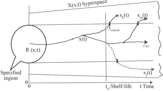
Let the parameters defi ning the product quality be xi(t) x ∊ (t) (i=1,2,..., n), e.g. content of water, acrylamide, intensity of some fl avour, which are solutions of eq. (5.1)a:
x(t) ∊ X(x; t). The x(t) phase vector moves in an R specifi ed region in X(x; t) hyperspace.
When an xi(t) parameter reaches the boundary of R, its value is xi, (ti,R). Thus, we obtain a series: x1, (t1,R), x2, (t2,R),... xi, (ti,R), ...xk, (tk,R ), etc. If tk,R is the smallest value in this series, i.e. the xk (t) parameter earliest reaches the boundary of R, then tk,R=tcritical is called a critical time-point, which defi nes the shelf-life as follows:
tsl < tcritical (5.9) Figure 1 shows that fi rst xk (t) leaves the R(x;t) region, then xl (t), then xm (t), etc. – but x0(t) never leaves the R (x; t) region. The region R (x; t), containing the permitted extreme (minimal or maximal) values of defi nitive product parameters, is defi ned by the product specifi cation prepared by the producer. The producer’s quality assurance system issues quality/veterinary/
fi tosanitary certifi cate to every lot of product, which proves that the actual lot meets the detailed requirements laid down in the product specifi cation.
Appendix shows a Monte-Carlo method for calculating the shelf-life.
Fig. 1. Shelf-life defi ned by the critical time-point in the way as tsl < tcritical.
6. The Third Law of thermodynamics
The Third Law relates to the behaviour of bodies approaching absolute zero temperature, but the research on the behaviour of complex materials in this fi eld is in initial stage compared to the studies of pure chemical compounds, see WUNDERLICH (2005). CHEN (1985) and others as DOMALSKI and co-workers (1986), CHOI and OKOS (1986), FRICKE and BECKER (2001), publish several specifi c thermal capacity data of cellular materials referring to –40 °C=233.15 K as deepest temperature, far from absolute zero temperature. Although relevant data are missing, it is reasonable to assume that the theory by Einstein, Debye, and Tarasov can be applied to the curve of specifi c heat capacity functions in case of complex materials as well. Similarly, the confi guration entropy of complex materials in proximity of zero absolute temperature might also become a future research topic. For more details see TARASOV (1945) and CALLEN
(1985).
7. Conclusions
The new model of thermodynamics expressed by this paper has some special features as follows:
– The complex materials have an essential, distinctive property: the polyagent behaviour.
– The polyagent behaviour leads to redundancy, macroscopic/microscopic uncertainties.
– Because of polyagent behaviour, some principal variables based on previous studies have to be chosen, which characterize the changes taking place in the complex materials.
– Because of the cellular structure, the Gibbs’ phase rule is not valid for complex materials, the degree of freedom cannot be determined for such systems, and the cellular equilibrium cannot be supposed in general.
– A real body has not a certain value of temperature because of its extend in space.
– The defi nition of Second Law is given in word: The real processes are irreversible. Its mathematical defi nition is given by a multivariant equation of time-development, which includes also the increase of entropy in direction of extremity.
– The specifi c thermal capacity (cV and cp) is defi ned as an apparent value in general because of the polyagent behaviour, and this is the base of calculating entropy differences, too.
– No suffi cient data on the specifi c thermal capacities and entropies in the proximity of the absolute zero temperature are available yet.
– In complex materials the traditional continuum physical approach cannot be generally used, instead of it, the dimensional analysis and the solutions of Rabinowitsch–Mooney equation are available, although they do not provide any information on dissipation in general.
– The shelf-life of foods is defi ned, and a Monte-Carlo method for its calculation is presented.
*
I express my thanks to Prof. Ferenc Firtha (Szent István University, Budapest-Gödöllő) for his help in programming the shelf-life calculation. Finally, I acknowledge the very valuable support obtained from my daughter, Viktoria Mohos Naray, for textual interpretation and editing.
Appendix
Monte-Carlo method for calculating the shelf-life of a product Principle:
During storage, the c concentration of an essential quality marker is randomly changing due to the t[s] time and the T[K] temperature. The model equation of c of a product is expressed by:
c=c1c2=exp(wt)×q×exp(–∆H/(RT)) (A1) where c1=exp(wt) expresses the ∆t duration at T temperature, c2=q×exp(–∆H/(RT)), w[s–1] is reaction velocity constant, c2 is an equation of Arrhenius-type, ∆H [J] is reaction energy, R [J/(molK)] is the universal gas constant, T [K] is the absolute temperature, and q is a constant of proportion. Although the molar mass is not relevant for complex materials, such Arrhenius- type equations are usually applicable to a virtual rate: ∆H/R. The value of c(t=0) is given:
c(0), and it holds c(0)=exp(0)×q×exp(–∆H/(R×298). In the following examples it is supposed:
∆H/R=400 K – this value has to be determined by previous studies. As a result it holds c(0)=2,718×q×exp(–400/298)=2.718×0.26125×q=0.71007×q.
The Matlab/Octave program is as follows:
Example 1: c(0)=f(0)=0.2, and this value is decreasing to f<0.05, i.e. 0.2=0.71007×q, and q=3.5504
Example 2: c(0) =f(0)=0.05, and this value is increasing to f>0.2, i.e 0.05=0.71007q, and q=14.2
Example 1 Example 2
x=1 x=1
for f=1:100 for f=1:100
r=exp(–400/(298+10×(0.5-rand))); r=exp(–400/(298+10×(0.5-rand)));
s=exp(–abs(0.5-rand)×0.6); s=exp(abs(0.5-rand)×0.6);
x=x×s x=x×s
f=(r×x)/3.5504 f=(r×x)/14.2
if f <0.05 if f>0.2
break break
end end
end end
After the program having run many times, the minimal value of product xi values provides the recommended shelf-life, taking into account the dimension ([1/month], [1/year]
etc.) of w (here in both examples: w=0.6): Πxi=exp[±(Σ∆t)×wi], i.e. ln(Πxi)=±(shelf-life)×w.
(The signs ‘+’ and ‘–’ relate to increase /Example 2/ and decrease /Example 1/, resp.) For Example 1, the minimum series obtained is: x=0.90454, f=0.066257; x=0.73929, f=0.053399; x=0.65289, f=0.047272. The product: 0.90454×0.73929×0.65289=0.43660, and ln 0.43660=–0.8287= –shelf-life×0.6/year, i.e. shelf-life=(0.8287/0.6) year=1.38 year=504 days.
References
AL-AZAWY, M.G., TURAN, A. & REVELL, A. (2017): Investigating the impact of non-Newtonian blood models within a heart pump. Int. J. Numer. Method. Biomed. Eng., 33, DOI: 10.1002/cnm.2780 (last accessed: 07 March 2018).
AMEND, J.P., LAROWE, D.E., MCCOLLOM, T.M. & SHOCK, E.L. (2012): The energetics of organic synthesis inside and outside the cell. Phylos. T. Roy. Soc. B., 368, (1622), 20120255.
BAGLEY, E.B. (1957): End corrections in the capillary fl ow of polyethylene. J. Appl. Phys., 28, 624–627.
BAGLEY, E.B., CHRISTIANSON, D.D. & MARTINDALE, J.A. (1988): Uniaxial compression of a hard wheat fl our dough:
Data analysis using the upper convected Maxwell model. J. Texture Stud., 19, 289–305.
BELOUSOV, B.P. (1959): Periodicheski deistvuyushchaya reaktsia i ee mekhanism (Periodically acting reaction and its mechanism) –in: Sbornik referatov po radiotsionnoi meditsine, 1958 (Collection of abstracts on radiation medicine, 1958) Medgiz, Moscow, pp. 145–147.
BELOUSOV, B.P. (1985): A periodic reaction and its mechanism -in: FIELD, R.J. & BURGER, M. (Eds) Oscillations and traveling waves in chemical systems. Wiley, New York, pp. 605-613.
BENEDEK, P. & LÁSZLÓ, A. (1965): Grundlagen des Chemieingenieurwesens. Deutscher Verlag für Grundstoffi ndustrie, Leipzig, Chapter VI., Section 5.
BOYCE, W.E. & DIPRIMA, R.C. (2012): Elementary differential equations and boundary value problems. 10th ed., John Wiley & Sons, WileyPLUS (Chapter 9), pp. 495–589.
CALLEN, H.B. (1985): Thermodynamics and introduction to thermostatistics. 2nd ed., John Wiley & Sons, Inc., New York, pp. 335–364.
CHEN, C.S. (1985): Thermodynamical analysis of the freezing and thawing of foods: Enthalpy and apparent specifi c heat. J. Food Sci., 50, 1158–1162.
CHOI, Y. & OKOS, M.R. (1986): Effects of temperature and composition on the thermal properties of foods. -in: LA
MAGUER, M. & JELEN P. (Eds) Food engineering and process applications, Vol. 1, Transport phenomena, Elsevier App. Sci. Pub., London, New York, pp. 93–101.
COGSWELL, F.N. (1972): Converging fl ow of polymer melts in extrusion dies. Polym. Eng. Sci., 12(1), 64–73.
COGSWELL, F.N. (1978): Converging fl ow and stretching fl ow: A compilation. J. Non-Newton. Fluid, 4, 23–38.
COGSWELL, F.N. (1981): Polymer melt rheology. Halsted Press, New York, NY, 180 pages.
DICKINSON, E. (1992): An introduction to food colloids. Oxford Science Publications, Oxford University Press, pp.
100–115.
DOMALSKI, E.S., JOBE, JR., T.L. & MILNE, T.A. (1986): Thermodynamic data for biomass conversion and waste incineration. A product of the Solar Technical Information program, prepared by the National Bureau of Standards under contract to the Solar Technical Information Program of the Solar Energy Research Institute (USA), Appendices A and B.
FRANKE, K. & TSCHEUSCHNER, H.D. (1991): Modelling of the high shear rate conching process for chocolate. J. Food
FRICKE, B.A. & BECKER, B.R. (2001): Evaluation of thermophysical property models for foods. Int. J. Refrig., 7, 311–330.
GIBSON, A.G. (1988): Converging dies. -in: COLLYER, A.A. & CLEGG, D.W. (Eds) Rheological measurements. Elsevier Applied Science, New York, NY, pp. 49–92.
GILBERT, E.N. (1966): Information theory after 18 years. Science, 152, 320–326.
GYARMATI, I. (1970): Non-equilibrium thermodynamics – Field theory and variational principles. Springer-Verlag, Berlin, Heidelberg, New York, Chapters II–III, pp. 17–87.
HELDMAN, D.R. (1975): Food process engineering. AVI, Westport, Connecticut, 401 pages.
HIRSCH, M.W., SMALE, S. & DEVANEY, R.L. (2004): Differential equations, dynamical systems, and an introduction to chaos. Elsevier, Chapter 14, pp. 230–231.
HOLLAND, B., WELCH, A.A., UNWIN, I.D., BUSS, D.H., PAUL, A.A. & SOUTHGATE, D.A.T. (1991): McCance and Widdowson’s – The composition of foods. 5th ed. Royal Society of Chemistry and MAFF. Cambridge, U.K.
LAPITOV, E.K. & FILATOV, B.S. (1963): Kolloidnüj Zhurnal, 25, 43–49.
LAROWE, D.E. & AMEND, J.P. (2016): The energetics of anabolism in natural settings. ISME J., 10, 1285–1295.
LASALLE, J. & LEFSCHETZ, S. (1961): Stability by Liapunov’s direct method with applications. Academic Press, New York–London, 514 pages.
LIU, G-T., WANG, X.-J., AI, B.-Q. & LIU, L.-G. (2004): Numerical study of pulsating fl ow through a tapered artery with stenosis. Chinese J. Phys., 42, 401–409.
LORENZ, E.N. (1987): Deterministic and stochastic aspects of atmospheric dynamics. -in: NICOLIS, C. & NICOLIS, G.
(Eds) Irreversible phenomena and dynamical system analysis in geosciences. D. Reidel Publ. Co., pp. 159–
179.
MACSIHIN, JU.A. & MACSIHIN, SZ.A. (1987): Élelmiszeripari termékek reológiája (Rheology of food industrial materials). Mazőgazdasági Kiadó, Budapest, pp. 221–229.
MATOLCSI, T. (2004): Ordinary thermodynamics. Akadémiai Kiadó, Budapest, pp. 11, 382–385.
MOHOS, F.Á. (1982): A kémiai technológiák szerkezetelméletének alkalmazása az édesipari gyakorlatban (The application of structure theory of chemical engineering in the confectionery practice). Cand. Theses, The Hungarian Academy of Sciences, Budapest.
MOHOS, F.Á. (1990): Édesipari technológia (Confectionery technology). Lecture notes, University of Horticulture and Food Technologies, Budapest, 266 pages.
MOHOS, F.Á. (2010): Confectionery and chocolate engineering – Principles and applications. Wiley-Blackwell, Oxford, UK, pp. 5–6, 12.
MOHOS, F.Á. (2017): Confectionery and chocolate engineering – Principles and applications. John Wiley & Sons, Ltd., 2nd ed., p. 4; Appendix 3., pp. 645–662.
REHER, E.-O., HAROSKE, D. & KÖHLER, K. (1969a): Eine Analyse der nicht-Newtonscher Reibungsgesetze und deren Anwendnung für die Rohrströmung. Teil I. Chem. Techn., Teil I: 21(3), 137–143.
REHER, E.-O., HAROSKE, D. & KÖHLER, K. (1969b): Eine Analyse der nicht-Newtonscher Reibungsgesetze und deren Anwendnung für die Rohrströmung. Teil II., I., Chem. Techn., 21(5), 281–284.
SCHRÖDINGER, E. (1967): What is life? The physical aspects of living cells. Cambridge University Press, Cambridge, U.K, Chapter 6, pp. 153–164.
SHANNON, C.E. (1948): A mathematical theory of communication. Bell Syst. Tech. J., 27, 379–423, 623–656.
Re-issued December, 1957: Monograph B-1598.
SMITH, E. (2008A): Thermodynamics of natural selection I: Energy fl ow and the limits on organization. J. Theor.
Biol., 252, 185–197.
SMITH, E. (2008b): Thermodynamics of natural selection II: Chemical Carnot cycles. J. Theor. Biol., 252, 198–212.
SMITH, E. (2008c): Thermodynamics of natural selection III: Landauer’s principle in computation and chemistry. J.
Theor. Biol., 252, 213–220.
STEFFE, J.F. (1996): Rheological methods in food process engineering. 2nd ed., Freeman Press, USA, pp. 110–121.
STROGATZ, S.H. (1994): Nonlinear dynamics and chaos. Addison-Wesley, Reading, MA, 498 pages.
SZILARD, L. (1929): Über die Entropieverminderung in einem thermodynamischen System bei Eingriffen intelligenter Wesen. Z. Phys., 53, 840–856.
TARASOV, V.V. (1945): The theory of the specifi c heat of high polymers, II. Rubber, graphite. Comp. Rend. Acad. Sci.
U.R.S.S., 46, 110–114.
TUSZYNSKI, J. & KURZYNSKI, M. (2003): Introduction to molecular biophysics, CRC Press LLC, 584 pages.
USDA (1975): Composition of foods. Agricultural handbook, 1975, No. 8, U.S. Departrnent of Agriculture, Washington, D.C., pp. 481–509.
USDA (1996): Nutrient database for standard reference, Release 11. U.S. Department of Agriculture, Washington, D.C.
USDA (1999): Nutrient database for standard reference, Release 13. U.S. Department of Agriculture, Washington, D.C.
VDI (1991): VDI-Wärmeatlas, 6th ed., VDI-Verlag, Düsseldorf.
VELASQUEZ, J.L. (2009): Finding simplicity in complexity: General principles of biological and nonbiological organization. J. Biol. Phys., 35(3), 209–221.
WUNDERLICH, B. (2005): Thermal analysis of polymeric materials. Springer-Verlag, Berlin, 894 pages.
ZHABOTINSKY A.M. & ZAIKIN, A.N. (1971): Spatial effects in a self-oscillating chemical system. -in: SEL’KOV, E.E.
(Ed.) Oscillatory processes in biological and chemical systems, Vol. II. Science Publ., Puschino. pp. 279–283.