DYNAMICS OF VISCOELASTIC BEHAVIOR Turner Alfrey, Jr., and E. F. Gurnee

C H A P T E R 11

DYNAMICS OF VISCOELASTIC BEHAVIOR Turner Alfrey, Jr., and E. F. Gurnee

I. I n t r o d u c t i o n 387 1. Volume Effects a n d Shear Effects 388

I I . Properties of Viscoelastic M a t e r i a l s 390 1. M e t h o d s of Specifying t h e T i m e - D e p e n d e n t Properties of Viscoelastic

Materials under Shear 390 a. T h e Voigt Model 390 b. T h e Creep F u n c t i o n 394

(1) T h e B o l t z m a n n Superposition Principle 394

c. T h e Maxwell Model 396 d. T h e Relaxation F u n c t i o n 397 e. T h e Mechanical Impedance F u n c t i o n 398

/ . T h e Complex Elastic Modulus 400 g. T h e Operator E q u a t i o n : Ps^ = 2Qe,-y 400 2. Relationships between t h e M e t h o d s 400

a. Voigt Model t o Creep F u n c t i o n 401 b. Maxwell Model t o Relaxation F u n c t i o n 401 c. Creep F u n c t i o n t o Voigt Model and t h e Similar R e l a x a t i o n F u n c t i o n

Transformation 401 d. Voigt Model t o Operator E q u a t i o n 402

e. Maxwell Model t o Operator E q u a t i o n 403 / . Operator E q u a t i o n t o Impedance F u n c t i o n 404 3. Viscoelastic R e p r e s e n t a t i o n s for Pressure-Volume Effects 405

4. Combinations of Volumetric and Shear Changes 405 5. Mechanical Models and Molecular Theories 408 I I I . Properties of Viscoelastic Objects when t h e D i s t r i b u t e d I n e r t i a of t h e M e -

dium is Neglected 413 IV. Vibrations and Waves in Viscoelastic Objects 417

V. T h e Kinetic T h e o r y of R u b b e r E l a s t i c i t y 423

Nomenclature 428 I. Introduction

A viscoelastic material is one which exhibits both elastic and viscous characteristics. Early interest in viscoelastic behavior centered around relatively simple phenomena, such as the relaxation of stress in glass or the creep behavior of pitch. Maxwell¹ demonstrated that some such materials can be adequately characterized by an elastic modulus and a viscosity,

1 Maxwell, J. C , Phil. Trans. Roy. Soc. 157, 49 (1867).

387

and developed the concept of the "relaxation time," which is the ratio of the viscosity to the elastic modulus.

More recent studies have shown that many substances (in particular, organic high polymers) cannot be characterized so simply. These more complex materials exhibit more than one relaxation time—or even a "dis- tribution of relaxation times." It is the purpose of this chapter to review the methods of specifying the properties of viscoelastic materials; to show how the strain (as a function of time) is related to the stress (as a function of time) for a material of specified properties; to comment briefly on the molecular mechanisms of viscoelastic response; and, finally, to analyze the dynamics of motion in viscoelastic objects, where the stress and strain are functions of position as well as of time.

This discussion will be limited to "linear" viscoelastic behavior, i.e., to cases where elastic effects follow Hooke's law and viscous effects are "New- tonian." In effect, this means a limitation to the region of small strains.

VOLUME EFFECTS AND SHEAR EFFECTS

The mechanical properties of an isotropic ideal elastic material can be specified by means of any two of several independent physical constants, i.e., the Young's modulus and the Poisson ratio, the Young's modulus and the shear modulus, or the shear modulus and the bulk modulus. It is, how- ever, convenient to resolve any strain into a change in volume with con- stant shape, plus a change in shape at constant volume. Consequently, if we use the shear modulus and the bulk modulus as the physical constants to represent the elastic properties, we are led to a simple mathematical separa- tion of pressure-volume effects from shear effects. Mathematically, the stresses and strains are tensors and are readily resolved into the sum of a

"mean normal" tensor and a "deviatoric" tensor, which represent the pure pressure-volume effects and the pure shear effects, respectively.²

We shall represent the stress tensor by the symbol σ*·,· : this symbolizes the entire set of stress components below:

σ\\ ση <τ\ζ\

ö"21 σ22 0"23 1 σ"3ΐ σ-32 σ 3 3 /

where ση , σ22, and σ33 are normal (or tensile) components, and σι2, ση , etc., are shear components. We shall represent the mean normal stress by the symbol σ.

ΟΊ1 + 0"22 + σ33 /-,Ν σ = 3 ^{( 1 )}

2 Love, A. E. H., "A Treatise on the Mathematical Theory of Elasticity." Dover, New York, 1944.

D Y N A M I C S O F VISCOELASTIC B E H A V I O R 389 The mean normal stress, σ, has the physical significance of a (negative) hydrostatic pressure. If we now subtract this "hydrostatic" term from the stress tensor (i.e., subtract σ from each of the three normal stress compo- nents), the residual tensor is designated as the deviatoric stress tensor, stJ-.

or

' β ι ι

«21

$12 $13 \

«22 $23 I ⁼

$32 $33/

S{j = (T{j

/ σ ι ι — σ 1 σ2ι

\ σ3ι

— σ-hij

σΐ2

0"22 — 0*

σ"32

^13

σ"23 σζζ — σ

(2) where δί;· = 1 for i = j and δί;· = 0 for i τ^ j .

The mean normal stress tends to alter the volume of the material; the deviatoric stress tends to alter the shape of the material.

Likewise, the strain tensor, ety, can be resolved into a mean normal strain (e), plus a deviatoric strain tensor, e^ .

0n

021 ,031

€11 + €22 + €33

€ = 3

012 ex\ /en — €

622 023 I ⁼ I ^€21

^32 0 3 3 / \ €31

e%j ⁼⁼ t%j € · Oij

€12

€22 — €

€32

€13

€23

€33 — €,

Or e2l 022 023 1 = I €21 €22 — € €2 3 I (3)

The mean normal strain, e, has the obvious physical significance of measur- ing the volumetric dilation of the strained material; in fact, e is just ^ of the fractional volumetric dilation. The deviatoric strain tensor, et-y, measures the shape distortion of the strained material.

We now come to the relation between stress and strain. The bulk modulus, B, governs the volumetric behavior; the mean normal strain is directly proportional to the mean normal stress.

σ = SBe (4) This is essentially a pressure-volume equation. Likewise, the shape deforma-

tion is determined by the shear modulus, G, which relates the deviatoric stress tensor and the deviatoric strain tensor (component by component):

Sll = 2Ö011 $12 = 2(?ei2 Sl3 = 2Gßiz\

s2i = 2(?e2i $22 = 2(?β22 e t c .

or

Sij = 2Gdj

When we procede to the analysis of viscoelastic materials, it will still be (5)

convenient to resolve the phenomena into volumetric effects and shape changes. We will immediately become concerned with time-effects. Thus the stress components and the strain components will be functions of time, and we will have to understand how the stress tensor (as a function of time) determines the strain tensor (as a function of time). This involved problem is somewhat simplified by the fact that the mean normal strain (as a function of time) is completely determined by the mean normal stress (as a function of time), and that each (time-dependent) component of the deviatoric strain tensor is determined by the corresponding (time-de- pendent) component of the deviatoric stress tensor.

II. Properties of Viscoelastic Materials

1. METHODS OF SPECIFYING THE TIME-DEPENDENT PROPERTIES OF VISCO- ELASTIC MATERIALS UNDER SHEAR^3-5

A linear viscoelastic material is defined as one which, under stress, gives a response that is a combination of linear elastic and linear viscous be- havior. Such materials are often represented by mechanical models which are designed to duplicate the observed time dependence. It should be kept in mind that these models give a description only of the phenomenological behavior of a sample and, in general, tell nothing of the detailed mech- anisms that underlie this behavior. We now procede to a discussion of some of these schematic representations as well as of other methods that have been used to describe the mechanical behavior of viscoelastic materials.

a. The Voigt Model

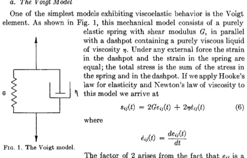
One of the simplest models exhibiting viscoelastic behavior is the Voigt element. As shown in Fig. 1, this mechanical model consists of a purely elastic spring with shear modulus (?, in parallel with a dashpot containing a purely viscous liquid of viscosity η. Under any external force the strain in the dashpot and the strain in the spring are equal; the total stress is the sum of the stress in the spring and in the dashpot. If we apply Hooke's law for elasticity and Newton's law of viscosity to

*\ this model we arrive at

where

s{j(t) = 2Geij(t) + 2veij(t)

deij{t)

(6)

ti3<t) =

FIG. 1. The Voigt model. dt

The factor of 2 arises from the fact that e»y is a shear component of a strain tensor and is equal to 3^ of the correspond-

DYNAMICS OF VISCOELASTIC BEHAVIOR 391 ing "classical" shear strain. The shear components of the strain tensor are defined as

1 (dUi_ , dUj\

2\dXj dXi)

where Ui and Uj are components of the displacement. Before the advent of tensor nomenclature, the "classical" shearing strains were simply defined as

dUi dUj dXj dXi

The shear modulus, G, was defined as the ratio of shear stress to (classical) shear strain. If we wish to use the tabulated values of shear moduli, we must introduce the factor 2, as shown in equation (6).

Throughout the text of this section, the simple term "stress" is used in place of the more cumbersome term "component of the deviatoric stress tensor." Likewise, the "corresponding component of the deviatoric strain tensor" is represented by the shorter term "strain." The subscripts in the equations should prevent any misunderstanding.

This equation is not sufficiently general to describe the observed mechani- cal behavior of complex viscoelastic materials such as high polymers. For example, if a material represented by equation (6) were subjected to a constant strain, the stress would remain constant, contrary to the usually observed stress relaxation. Furthermore, if the Voigt model is subjected to a constant stress, s0, the solution of equation (6) is

Again, this simple exponential increase of strain under constant stress is not observed except in particularly simple cases.

It should be noted that the quantity η/G has the dimensions of time, and it is defined as the retardation time, λ, of the Voigt element. The sig- nificance of the retardation time is brought out clearly by considering a creep recovery experiment. In such an experiment the load is suddenly re- moved from a creep specimen, and the strain diminishes. In the case of a Voigt element, this strain decay follows a simple exponential relation with time, and the retardation time, λ, becomes the time required for the strain to fall to 1/e of its original value.

It will further be seen that the retardation time, as the ratio of η to (?,

3 Alfrey, T., "Mechanical Properties of High Polymers." Interscience, New York, 1948.

4 Alfrey, T., and D o t y , P. M., / . Appl. Phys. 16, 700 (1945).

6 Gross, B., "Mathematical Structures of the Theories of Viscoelasticity.^{, ,} Her- mann, Paris, 1953.

will be short, i.e., the strain recovers fast, if 77, which characterizes the

"internal" friction, is small compared to the rigidity modulus, G. Vice versa, preponderance of the internal friction, 77, will retard the strain re- covery greatly and the retardation times will be long. The viscosity, 77, associated with the Voigt body is often referred to as "internal" viscosity because it relates to the internal friction which delays, but not prevents, the complete deformational recovery of a material which thus is essentially a solid.

In order to extend the Voigt model into a more realistic system for de- scribing viscoelastic behavior, it is convenient to consider a set of N Voigt elements connected in series as shown in

—I Fig 2. The nth element is composed of a modulus Gn and a

|_lj n viscosity ηη ; consequently it has a retardation time λη =

— Vn/Gn . It is assumed that no two elements have the same I rjj retardation time; any two elements that did have the

2 T , I ² same retardation times could always be replaced by a r—■—I single equivalent Voigt element.

G3 i LU η 3 The standard Voigt model of Fig. 2 represents a visco-

; elastic solid] that is, the material does not exhibit un- limited, nonrecoverable viscous flow. However, if one of ί Π . the Voigt elements is given a zero modulus, the element

n f 1 ^^η degenerates to a simple dashpot, which does undergo

; unlimited, nonrecoverable viscous flow. A Voigt model

C

l—. containing such a degenerate element corresponds to a vis- [1] r\N coelastic liquid. Another form of degenerate Voigt element I—' is that with a zero viscosity (an unretarded spring). The j inclusion of such an element in a Voigt model corre- F 2 Th ^sPOⁿds to a certain amount of instantaneous elastic com- generalized pliance in the material.

Voigt model. Since this system is connected in series, all elements are under the same stress, Sij(t). Thus, for the nth element

Sij(t) = 2GneiKn)(t) + 2ι?ηβίχ«)(0 (8)

In addition, the total strain will be given by the sum of the strains in the individual elements. Thus

e<s(t) = Σ eij(n)(t) (9)

n=-l

The N differential equations represented by equation (8)—(n = 1· · -N)—

and equation (9) completely determine the mechanical behavior of the model shown in Fig. 2. It should be noted that the individual strains,

etj(n)(t), are not observable quantities; they are important only as a means of relating Sij(t) and β»>(0·

DYNAMICS OF VISCOELASTIC BEHAVIOR 393 One of the simplest types of experiment for studying viscoelastic be- havior is the creep test, in which a stress is suddenly imposed on the sample at time zero, and then maintained constant. The time-dependent strain response to this steady stress is called the creep curve.

If this system of N Voigt elements is suddenly subjected to a constant stress, So, the solution of equation (8) gives the strain in the nth element as

and consequently

e«/(n)(0 = 2 ^JnSo ! ~ ^{e x}P ( - Γ - ) (¹⁰)

e«(0 = |° Σ Jn [ l - exp ( - £ ) ] (11) Here we have replaced the modulus Gn by the compliance Jn = 1/Gn .

Equation (11) is a better representation of observed viscoelastic creep than equation (7) since it contains more parameters and consequently is more general. Also, if the strain, e,-y(i), is held constant, equations (8) and (9) are consistent with a stress relaxation, although this is not a convenient mathematical approach to this problem.

In the limit N —> oo, we have an infinite set of elements over which the retardation times may range continuously from zero to infinity. The finite set of constants (λη , Jn) is replaced by the function J(X), which gives the amount of elastic compliance associated with the retardation time, λ.

It is often referred to as the "distribution of retardation times," while in fact it is a distribution of compliance.

Equation (9) is now written as

/»oo

e*i(0 = / eat, λ) d\ (12)

Jo

For the case of constant stress, s0, the strain, etJ(£, λ) is given by

ea(f, λ) = | J(X) [ l - exp ( - 0 ] (13) and consequently

e

i}

(t) = |° [ J(\) [l - exp ( - 0 ] d\ (14)

It should be noted that this discussion has implicitly introduced another method for describing viscoelastic materials, namely, by the specification of the distribution function J(\). This method is so closely related to the generalized Voigt model that it is not listed as a separate representation.

One of the characteristics of a linear viscoelastic material, which is il-

lustrated by the Voigt model, is the fact that it obeys the Boltzmann superposition principle. This principle has its important applications in the discussion of creep functions and relaxation functions as indicated later. It may be briefly summarized by stating that if a material is subjected to a series of known stresses, the net effect on the strain is the sum of the effects of each of the individual stresses.

b. The Creep Function* ·⁷

If a relaxed viscoelastic material is suddenly subjected to an instantan- eous constant stress, sa(t) = s⁰, equation (14) gives the strain as a function of time. Since stress-time (creep) experiments are very convenient, it is useful to define a (shear) creep function by

*>(0 = ^ (15)

So

which essentially defines a strain per unit stress. It is related to the set of Voigt model equations through the function J(\) in the case of an infinite set of elements, and through the constants (Jⁿ , λΛ) for a finite set.

There is an important mathematical difference between the creep func- tion and the corresponding expression for a set of Voigt elements. The Voigt model represents a set of differential equations, whereas the creep function is merely one particular solution to these equations, namely, the solution for constant stress. The differential equations can be directly applied to any stress sequence, s^t-y(Z); the creep function can be applied to time-dependent stresses only indirectly, through the Boltzmann super- position principle.

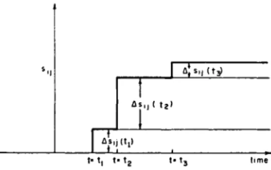
(1) The Boltzmann superposition principle.⁶'⁷ This important principle, as applied to creep experiments, states that the strain at any time t, because of the previous application of several stresses in succession—i.e., the stress is a sequence of step functions—is the summation of the strains that would be observed at that time if each of these constant stresses had been applied independently.

Thus, if the applied stress is given by the function shown in Fig. 3, then the strain at the time (t) is given by

2e<y(i) = As^hMt - h) + As^tj(^{t - h) + As^tj(U)<p(t - U) (16) Each term in this sum represents the contribution to the strain at time (t) from a particular stress increment.

By means of this principle, it is possible to determine the strain as a

6 Leaderman, H. "Elastic and Creep Properties of Filamentous Materials and other High Polymers." Textile Foundation, Washington, D. C , 1943.

7 Leaderman, H., Ind. Eng. Chem. 35, 374 (1943).

DYNAMICS OF VISCOELAST1C BEHAVIOR 395

*■! 1 ^S l J( t 3 )

1

A s , , ( t2)

— L i j . . . ».

t» t, t« t2 t - 13 time

FIG. 3. Stress as a sequence of step functions.

O f t time

FIG. 4. Stress as an arbitrary function of time.

function of time when the complete stress history and the creep function are known. For example, assume that the stress as a function of time is given, as shown in Fig. 4, and that we are interested in determining the strain as a function of time. The stress increments are now determined from the slope of the stress curve, and the summation is replaced by integration. Hence the strain as a function of time is determined by the integral

2e

_y

(«) = ]%«-<') ^ '

(17) In principle, this integral can be treated as an integral equation to give the stress as a function of time if the strain as a function of time is known, although in general the mathematical difficulties will be objectionable. In the particular case in which the strain is a constant, the transformation of equation (17) gives the stress as a function of time in terms of the creep function and the strain as a parameter, i.e., a method of relating the creep function and the relaxation function.⁵'⁸

8 Simha, R., J. AppL Phys. 13, 201 (1942).

c. The Maxwell Model

Another simple model used to describe viscoelastic behavior is the Max- well model (Fig. 5) consisting of a spring (modulus (?) and a dashpot (vis- cosity η) in series. In such a model, the total strain observed is the sum of a strain in the spring and a strain in the dashpot, while the stress in the spring and the stress in the dashpot are equal. The fundamental differential equation governing this model is

2e_iS(t) = - suit) + ί SiAt)

η Or

If the Maxwell model is subjected (suddenly, at time t strain e^ = eo, the solution of this equation is

Sij(t) = 2edG e x p

( - ; )

(18) 0) to a constant

(19) where η/(?, the relaxation time for the system, has been replaced by the sumbol r. As can be seen from equation (19), the relaxation time, r, is equal to the time required for the stress to relax to 1/e of its initial value when the strain is held constant.

It is possible to generalize this model in a manner analogous to that indi- cated above for the Voigt representation—first to a system of N parallel Maxwell elements as shown in Fig. 6, and then to an infinite set.

The relationship between stress and strain for the nth element in Fig. 6 is given by

2βΌ·(0 = — e*i(n)(0 + -FT e<i(n)(Ö

Vn On

(20)

F I G . 5.

,ψη ₂ ψ

F I G . 6.

FIG. 5. The Maxwell model.

FIG. 6. The generalized Maxwell model.

DYNAMICS OF VISCOELASTIC BEHAVIOR 397 and the total stress is

N

8<M = Σ sij(n)(t) (21)

n«=l

If this system is suddenly subjected to a constant strain, et-y(<) = e0, the stress, Sij(t), can be written as

Sijit) = 2e0 Σ Gn exp ( - - ] (22)

n - l \ rn/

For an infinite set of Maxwell elements the constants (Gn , rn) are replaced by the function G(T), which gives the amount of elastic modulus associated with the relaxation time, r. This function is often referred to as the "dis- tribution of relaxation times." The total stress, s,-y(i), is given by

8tj(f) = f 8ij(f, r) dr (23) Jo

For the case of constant strain, e^(£) = e0, the stress, Sij(t, r), is given by

* A T ) = 2edt?(r)exp(-M (24) and consequently

e*y(<) = 2e0 f G(T) exp ί - - J dr (25) d. TAe Relaxation Function

If a relaxed viscoelastic material is suddenly subjected to a constant strain, e#(£) = e0, the stress at any time is proportional to this strain, and is given by the formulas discussed under the section on Maxwell models.

Following the reasoning used in the discussion of the creep function, we find it convenient to define a relaxation function as the stress per unit strain. Thus

*(t) =

^Sj

ß (26)

2β0

From equation (25) it is readily seen that the relaxation function can be written as

ψ(0 = /o° ° G ( r ) e x p ( ' - i ) d r (27) In order to make use of the relaxation function when the strain, e^(i), is a

function of time rather than a constant, it is necessary to employ the Boltzmann superposition principle. In a manner similar to that discussed under the creep function, it is readily shown that from a given strain func- tion, e,-j(i), the stress as a function of time is found to be

Sii(t) = 2

[j ^{t ~ ^t,)d w ^dt '

⁽²⁸⁾

By means of this equation, the relaxation function can be used as a per- fectly general representation of viscoelastic materials.

e. The Mechanical Impedance Function

There is a close mathematical similarity between the mechanical response of a viscoelastic material and the electrical response of a two-terminal electrical network. Electrical-mechanical analogies of several different types can be developed, but the most felicitous choice of "corresponding"

variables is shown in Table I. If this correspondence is used, series coupling of two elements in a mechanical model must be replaced by parallel coupling in the corresponding electrical network in order to achieve mathematical identity; likewise, parallel coupling in the mechanical model corresponds to series coupling in the electrical network.³

TABLE I

ELECTRICAL MECHANICAL

Quantity of Electricity E.M.F. ( E )

Current ( I ) Capacitance

(C) £

Resistance

(R) {

P a r a l l e l Coupling Series Coupling

Φ

Strain ( 2 e j j ) Stress ( s j j )

/ cJe ί ■ \ Rate of Strain ( 2 ——*-J dt Compliance

(J) I

Viscosity

Series Coupling

P a r a l l e l C o u p l i n g

DYNAMICS OF VISCOELASTIC BEHAVIOR 399 Our interest here is not in the mechanical-electrical analogy as such;

we are interested in the concept of impedance, which has been so successfully used in the mathematical analysis of electrical networks, and which can be translated into mechanical terms.

The electrical impedance is most simply introduced in connection with the steady-state response to a sinusoidal voltage.

E = (R[£0 exp (ζωί)]

(29) / = (R[Jo exp (i[ut + φ])]

where (R represents the real part of the complex quantity. The impedance, Z, is a complex number which defines the relative phase as well as the relative amplitude of the current (relative to the voltage).

z = EQ exp (ίωί) φ φ

I0 exp [i(o)t + φ)]

Just as in the electrical case, the mechanical impedance is & function of fre- quency, and is hence often written as Ζ(ω). A discussion of the frequency dependance in molecular terms will be found in Section II-5.

The corresponding mechanical case (steady-state response of a visco- elastic material to a sinusoidal stress) involves the following equations:

Sij(t) = (R[SQ exp (iot)]

2e»y(0 = (R[2e0 exp (i[co* + <p])]

„ , v so exp (icoO (31)

2e0 exp (i[co£ + φ])

For example, the impedance function for a single Voigt element, with com- pliance J and viscosity η, would be

Ζ(ω) =η-—τ (32)

Although the impedance function is defined in terms of steady-state re- sponse to sinusoidal loading, it can be used to relate st-y(i) and β»·7·(ί) in more general stress sequences, by the use of Fourier transforms. Equation (31) will apply to each Fourier component of the stress and strain. Thus,

25^:Κ·(0]

where $[sij(t)] represents the Fourier transform:

$[8iM] = ί satt) exp ( - t « Ö dt (34)

J— 00

/. The Complex Elastic Modulus

Closely related to the complex mechanical impedance, Ζ(ω), is the complex elastic modulus, (?*(ω). Whereas Ζ(ω) relates the stress and the rate of strain (for steady-state sinusoidal loading), (?*(ω) relates the stress and the strain (for a similar steady-state experiment).

Sij(t) = So exp (ίωΐ)

2β»·/(ί) = 2e0 exp [ifat + <p)]

n*, x So exp (ίωί) So , · · \ 2e0 exp |ζ(ω£ + <p)J 2e0

(35)

The in-phase component of equation (35) is sometimes referred to as the dynamic modulus⁹ and the other component is called the dynamic loss. The knowledge of the frequency dependence of these two components, i.e., a knowledge of the complex elastic modulus at all frequencies, completely describes the viscoelastic material.

g. The Operator Equation: Pstj = 2Qet;

We have discussed viscoelastic representations that are particularly suited to studies involving known Sij(t) (Voigt models, creep function), those that are useful under conditions of known eu(t) (Maxwell models, re- laxation function), and those that are convenient to use under conditions of periodically varying stress and strain (mechanical impedance function, dynamic modulus). The operator equation method, which will now be de- scribed, is probably the most general method in the sense that it does not favor any particular form for the stress or strain; this equation is given by

P8a(t) = 2Qea(t) (36) where

~.m r*m—1

p

-ifr + *^b*

⁺

---

⁺

»

⁽³⁷⁾

Q = <Zn£+ ··■ +?o (38)

The parameters p and q characterize the viscoelastic material; their sig- nificance is brought out in the discussion of the relationship between the operator equation and the various models.

2. RELATIONSHIPS BETWEEN THE METHODS^3-5

Since any of the above methods can be used to describe a viscoelastic system it is useful to investigate the relationships between these methods,

9 ''Dynamic modulus" has also been used to represent the magnitude of the

1 'complex elastic modulus."

DYNAMICS OF VISCOELASTIC BEHAVIOR 4 0 1

i.e., techniques for converting from one representation to another. In the first place, it should be noted that the number of arbitrary constants needed to describe a viscoelastic material will be the same for all methods of representation, although the arrangement and magnitude of these con- stants will differ considerably from one method to the other. Consider a system of N Voigt elements, corresponding to a set of N differential equa- tions, each involving two constants. If the same system is described with the operator equation, 2N constants are also needed, but this time they ap- pear as 2N coefficients of one differential equation of higher order.

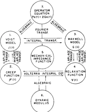
The mathematical relationships between these different methods have been discussed in detail by other authors.3 - 5·8·1 0 Here we will be content with a diagram summarizing the methods used (Fig. 7) and a brief discus- sion of the more important transformations.

a. Voigt Model to Creep Function

From a given \^roigt model, the creep function is obtained directly from equations (14) and (15).

b. Maxwell Model to Relaxation Function

In a similar manner, a set of Maxwell elements suddenly subjected to the constant strain e0 would show a stress decay of

8ij(t) = 2e0 f G(T) exp (--)dr

and hence

Mt) -/föMexp^-^dr

Thus, for any given distribution function (?(τ), it is relatively simple to determine the corresponding relaxation function.

c. Creep Function to Voigt Model and the Similar Relaxation Function Transformation

This transformation is usually more important than a and b above, since it provides a method of obtaining a theoretically useful quantity, J(X) or G(r), respectively, from the experimentally determined creep function or relaxation function. If \p(t) is known, the function G(r) can be obtained by an inverse Laplace transformation, and a similar relation holds between J and <p(t). In actual practice, however, the functions \p(t) and <p(t) are known only over a limited range of the variable, and as an additional com- plication, they usually cannot be represented by simple analytic functions.

10 Alfrey, T., Quart. Appl. Math. 3, 143 (1945).

FIG. 7. Relationships between the various representations.

Approximate methods have been developed for carrying out this trans- formation;^{11, 12} they essentially involve plotting the stress or strain as a function of log t and then taking the slope of this curve. Further approxima- tions, involving higher derivatives of the functions ψ(ί) and <p(t) have also been discussed.¹³·¹⁴

d. Voigt Model to Operator Equation

A new method will now be described which gives the transformation from a Voigt model to the operator equation. At the same time, several interesting properties of the operator equation will become apparent. For simplicity, the ij subscripts have been omitted from the next six equations.

Consider a system of (n + 1) Voigt elements, the first n of which are described by the operator equation

Ps = 2Qei (39)

11 Ferry, J. D., Sawyer, W. M., Browning, G. V., and Groth, A. H., / . Appl. Phys.

21,513 (1950).

12 ter Haar, D., Physica 16, 738 (1950).

" Andrews, R. D., Ind. Eng. Chem. 44, 707 (1952).

14 Schwarzl, F., and Staverman, A. J., Appl. Set. Research A4, 127 (1953).

DYNAMICS OF VISCOELASTIC BEHAVIOR 403 The operator equation for the (n + l)th element is simply

s = 2Ge2 + 2ηέ2 (40)

and the total strain is

e = ei + e2 (41)

Elimination of e2 from equations (40) and (41) results in

ei = e + 1 e - JL - | e i (42)

which permits equation (39) to be written as

ft

-»(' + 8'-»-3*)

But if D = d/dt, then

DPs = 2i)Qei|

= 2QA J

Therefore, for this system of (n + 1) Voigt elements, the operator equation (43)

(44)

IS

(p + | DP + I Qj

Sij

= 2

( Q

+ | DQJ e

(i

(45)

By inductive reasoning it can now be shown that all of the coefficients in the operator equation are positive. In addition, the roots of the operator Q are the negative reciprocals of the retardation times of the individual Voigt elements. For

(I + J B ) - O

Qll+%D) = 0 (46) has the (n + 1) roots D = — G/TJ, which is — 1/λη+ι, and the n roots of

Q = 0, which are the negative reciprocals of the first n retardation times by the inductive assumption.

Equation (45) also presents a rapid method for writing down the operator equation for a given Voigt model. By starting with n = 1 and applying equation (45) it is possible to write down the operator equation quite rapidly for relatively simple systems.

e. Maxwell Model to Operator Equation

By following the same procedure as described above it is possible to write a generalized operator equation for (n + 1) Maxwell elements, and use it

to make this transformation. In this case the roots of the operator P are the negative reciprocals of the relaxation times.

/. Operator Equation to Impedance Function

The shear mechanical impedance function is defined as

7( x S[8ij(t)] , .

ζ(ω) =

mm ⁽⁴⁷⁾

where the Fourier transform fF is given by

0=1/(0] = ί f(t)-exp(-iiot)dt (48)

J—oo

The operator equation can be written as

Psi3{t) = 2Qeij(t) (49)

or

Σ pmD^mSij(t) = 2 Σ qnDⁿeij(t) (50)

m n

The relationship between equations (47) and (50) is readily found by means of the identity

ff [£/«)] = M

ⁿ

s[/(01 (si)

and the linear property of SF.

If we apply the transform operation to each term in equation (50), we arrive at

Σ PmduT-ZisiAt)] = Σ qn(iü>y-$[2eij(t)] (52)

m n

But from equations (47) and (51) we have

Λ(ω) = —— (53;

(*ωΜ2^·(0]

and consequently

Σ qn{ioi)ⁿ

Ζ(ω) =

Γ Τ Τ Τ τ '

⁽⁵⁴⁾

m

Thus, given the shear operator equation, the shear mechanical impedance function is given directly by equation (54). This last equation can be manipulated by simple algebra into the form

Ζ(ω) = (RZ(co) + ίϋΖ(ω) (55)

DYNAMICS OF VISCOELASTIC BEHAVIOR 405 The real part, (R, and the imaginary part, ύ, are functions of ω and the various qn's and pn's. Since this "simplification" leads to fairly cumbersome expressions, equation (54) will be found more useful.

3 . VlSCOELASTIC REPRESENTATIONS FOR PRESSURE-VOLUME EFFECTS

The methods of representing viscoelastic materials described above have assumed pure shear stresses on the sample. In the case of pressure- volume changes, analogous models can be used although in this case the moduli and viscosity in the models do not have the same values as those for shear. The coefficients in the operator equation will therefore be dif- ferent ; this equation for these bulk changes is conveniently written as

P'a(t) = 3Q'e(t) (56) (The factor of 3 arises from the fact that the tensor notation of equation

(56) expresses the linear change in a pressure-volume experiment which is ^ of the fractional volume change used to define the classical bulk modulus.)

There is one major difference between pressure-volume effects and shear:

in bulk changes it is impossible to have unlimited viscous flow. If such were possible, then continued application of a compressive force would result in continually increasing the density of the material. This absence of viscous flow implies the following restrictions on the common models:

Voigt—there can be no free dashpot in the Voigt model.

Maxwell—there must be a free spring in the Maxwell model.

Operator equation—the coefficient go cannot be zero.

4. COMBINATIONS OF VOLUMETRIC AND SHEAR CHANGES

Once the behavior of the material is known under compression and shear it is possible to calculate the behavior under any combination of stresses.

This is the result of the fact that any stress may be expressed as a com- bination of shear and compression. The easiest method for this mathemati- cal manipulation is by means of the operator equation and tensor notation.

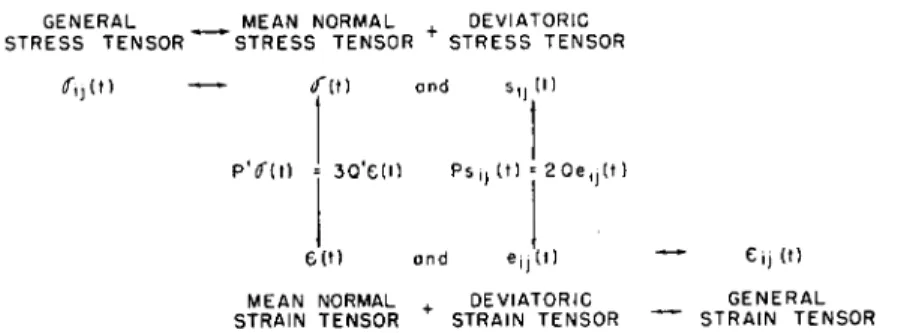
The general scheme is indicated in Fig. 8. Any stress or strain tensor can be decomposed into the sum of a mean normal tensor and a deviatoric tensor.¹⁵ The mean normal stress and strain tensors are related by the operator equa- tion for compression, and the deviatoric tensors by the shear operator equation. The arrows in Fig. 8 can be used in either direction.

The net result in the case of simple tension is the equation

P'VnW = Q"en(0 (57) where P " and Q", the operators for tension, are expressed in terms of

16 Alfrey, T., Quart. Appl. Math. 2,113 (1944).

GENERAL MEAN NORMAL DEVIATORIC STRESS TENSOR STRESS TENSOR STRESS TENSOR

^ i j ( t ) — * <T{\) and Sjj

P Y ( t ) ■■ 3 0 ' e ( t ) P s j j ( t )

6 ( t ) ond ejj MEAN

STRAIN

(t)

2 0 e j j ( t )

(t) NORMAL . DEVIATORIC TENSOR STRAIN TENSOR

— e j j ( t ) GENERAL

~ STRAIN TENSOR

FIG. 8. Scheme showing relation between a general stress tensor and a general strain tensor.

P', Q', P, Q. As an example of the method outlined in Fig. 8, we will actually evaluate P" and Q". In order to obtain a more complete visualization of this process we will write out the tensor components in array form. The stress tensor is written as

aij(t) or

(ση{1) 0 0\

0 0 0

K 0 0 0/ (58) for a tensile stress in the first direction.

The mean normal stress is Y^ of the sum of the diagonal terms of the stress tensor, and the mean normal stress tensor is this scalar multiplied by the unit tensor. Thus

/ l 0 0\

or ^σιι(θ(θ 1 0

\0 0 1)

σ(0 or Vsan(t)[0 1 0 ) (59)

By subtracting these tensors, the deviatoric stress tensor is found to be /%ση(0 0 0 \

Sij(t) or I 0 -HMO 0 (60)

\ 0 0 - M * i i ( 0 / In a similar manner we can write down the following strain tensors:

€tf(0 or

<o

or

/ I 0 (^

H(«n + «22 + en)[ 0 1 0

\o o i>

(61)

(62)

DYNAMICS OF VISCOELASTIC BEHAVIOR 4 0 7

(

%en — 3^€22 — M^€33 0 0 \

0 %€» - Heil - 3^633 0 (63) 0 0 %€33 — 3^11 — 3^3622/

where en , e22, and €33 are various functions of time.

The operator equation for volumetric changes relates expressions (59) and (62) to give

ΗΡ'σκ® = Q'(eⁿ + e22 + e33) (64) The operator equation for shear leads to the three equations

%Ρση(ί) = 2Q(%eⁿ - H*a - He») (65)

-ΜΡσκΟ) = 2Q(%€» - H«u - ^€33) (66) - H * W 0 = 2Q(^€33 - Hen - He») (67) The combination of the last two equations leads to the result €22 = €33.

The elimination of €22 and €33 from equations (65) and (66) gives the desired operator equation relating an(t) and en (t), namely

(3QP' + Q'P)aⁿ(t) = 9QQ'€ii(0 (68)

Thus

P " 3Q'P + QP'

Q" 9QQ' (69)

This last equation is simply an extension of Young's modulus for the elastic case to an operator for the viscoelastic case. It has a mathematical form that is quite similar to the expression for Young's modulus in terms of shear modulus and bulk modulus. That is, for the elastic case we have

«-BTS

⁽⁷⁰⁾

If we make the reasonable substitutions

»-?

in this equation, the final simplified result is equation (69). In practical

applications, as we shall see later in this chapter, this substitution procedure will prove extremely useful.

In many cases the material can be considered incompressible, and the mean normal strain will be zero. The only time dependence will arise from the shear (i.e., the deviatoric stress tensor). This presents certain simplifi- cations w^Then proceding from the stress tensor to the strain tensor. The reverse direction, from a given strain to a given stress, is impossible, since the mean normal stress is indeterminant. As far as time dependence is con- cerned, however, it is not necessary to procede further than the deviatoric stress tensor.

5. MECHANICAL MODELS AND MOLECULAR THEORIES

We have seen that the properties of a viscoelastic material can be de- scribed in various different but equivalent ways. Two of these modes of de- scription involve mechanical models (the Voigt model and the Maxwell model). It should be emphasized that the use of such models does not neces- sarily imply anything concerning the molecular mechanisms responsible for

the observed behavior. Voigt and Maxwell mod- els can be used in a completely phenomenological treatment of viscoelastic response. When this is the intention of the writer, the model must be interpreted as being a pictorial symbol which represents a set of differential equations. Thus, the Voigt model of Fig. 9 represents the set of equa- tions:

\ ,

ώ

Sij(t) = 2Giei^ja) (t)

Sij(t) = 2G²eij(2)(t) + 27?²e\y⁽2)(0 Sij(t) = 2τ7³6ϋ(3)(0

e.ij(t) = e^ij(i)(t) + e^ijm(t) + e^ij{Z)(t) (71)

FIG. 9. A four-para- meter Voigt model.

Furthermore, in a rigidly phenomenological treat- ment, the individual strain "contributions" e^t-y(i)(0>

eH(2)(t), and eij(z)(t) must be recognized as beingun- observables. The aim of a phenomenological theory of viscoelasticity is to connect one set of observable mechanical functions of time [the stress com- ponents Sij(t)] with another set of observable time functions [the strain components e^t-y(i)]. In the Voigt model approach, this mathematical con- nection is made by a calculation which introduces and utilizes, but then discards, a set of unobservable quantities (the contributions e»j(n)(£) to the strain components). Likewise, the Maxwell model approach utilizes a set of unobservable stress contributions, «</(«) (0> ^m the intermediate stages of

DYNAMICS OF VISCOELASTIC BEHAVIOR 409

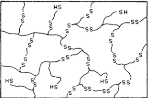
FIG. 10. Polysulfide rubber chain structure.

the calculation. Such use of unobservable quantities in the intermediate stages of a calculation is a perfectly valid device, often employed in theo- retical physics. As long as the phenomenological unobservability is recog- nized, there is no valid objection to this type of procedure; in particular, there is no valid objection to the use of mechanical models in a phenomeno- logical treatment of viscoelastic behavior.

A sound phenomenological analysis, however, is only the first step in a.

completely satisfactory understanding of any physical phenomenon of the type under discussion. The next, and more difficult, step is the elucidation of the molecular mechanisms involved. When an attempt is made at develop- ing a molecular theory of viscoelastic behavior, the mechanical ' 'models'' discussed earlier take on a new significance. In certain simple cases, the individual elements of a Voigt or Maxwell model can be confidently identified with definite processes on the molecular level. (See the following para- graphs for illustrations of such cases.) Usually this is not true. The existing molecular theories are so crude that we are usually able to give, at best, a very qualitative and tentative mechanistic interpretation of the elements of the phenomenological model. This does not mean that we should avoid molecular interpretations in the case of complicated substances. It does mean that we must recognize the tremendous gap between the present states of phenomenological theory and molecular theory of viscoelastic behavior; and that we should indicate clearly, when using mechanical models, whether we are making rigorous phenomenological statements or speculative mechanistic statements.

Let us now consider a few simple cases where the molecular mechanisms of viscoelastic response seem fairly clear, and then examine the less success- ful attempts to develop more general molecular theories.

Tobolsky and co-workers¹⁶'¹⁷ have studied the molecular mechanism of I⁶ Mark, H., and Tobolsky, A. V., "Physical Chemistry of High Polymeric Sys- tems." Interscience, New York, 1950.

"Tobolsky, A. V., Prettyman, I. B., and Dillon, J. H., J. Appl. Phys. 16, 380 (1944); Stern, M. D., and Tobolsky, A. V., J. Chem. Phys. 14, 93 (1946).

stress relaxation in polysulfide rubber. This material is a network polymer, with disulfide links in the polymeric chains of the network, and with a cer- tain number of mercaptan terminal groups on the linear "tails" which are attached to the network. This structure is indicated schematically in Fig. 10. This network polymer exhibits rubberlike elasticity. When a sample is stretched, the chains which constitute the network are forced from their original random distribution of configurations into a new distribution of lower entropy. The equilibrium elastic properties of such a network are reasonably well understood (see refs. 3, 18). This purely mechanical response is, however, complicated by a concurrent chemical reaction, namely, the mercaptan-disulfide interchange reaction. Each time this reaction occurs, one disulfide bond is broken, and one new disulfide bond is formed:

The net effect of this balanced scission-crosslinking reaction on the poly- mer structure is nil, when the sample is in the unstrained state. In a stretched sample, on the other hand, this scission-crosslinking reaction results in a decay of the stress. This is so because when a chain which is under tension is cut, it is replaced by a new network-chain which is in a relaxed configura- tion. The over-all effect is that this type of material exhibits Maxwellian relaxation behavior. The elastic modulus (spring of the Maxwell element) is explainable in terms of the kinetic theory of rubber elasticity; and the relaxation time is governed by the chemical kinetics of a definite, specified chemical reaction.

This same general molecular concept has been applied qualitatively in other cases, and has been extended (qualitatively) to explain the properties of materials which exhibit a distribution of relaxation times. The logic of such an expanded treatment goes roughly as follows: "The structure is held together by forces of many different types: weak van der Waals' forces, dipole-dipole interactions, hydrogen bonds, labile covalent bonds, and stable covalent bonds. These bonds will break and reform, at different rates.

If the sample is held in a deformed shape (e.g., at constant tensile strain), the bond breaking and reforming will result in stress relaxation. The pres- ence of bonds of different strengths (and hence different rate constants for breaking and reforming) results in a distribution of Maxwellian relaxation times, rather than a single sharp relaxation time."

The weakness of such an extended "theory" of the Maxwellian relaxation distribution is that it involves many ad hoc assumptions. At the present

» Treloar, L. R. G., "The Physics of Rubber Elasticity." Oxford, New York, 1949.

DYNAMICS OF VISCOELASTIC BEHAVIOR 411 time, it is not possible to actually predict the relaxation distribution from the molecular structure by introducing independently measured rate con- stants for the various scission and crosslinking processes involved.

Let us now consider briefly those molecular theories which have been formulated in terms of the Voigt model. This type of theory has been principally applied to amorphous linear high polymers, such as polystyrene.

A crude, qualitative representation of the viscoelastic behavior of such a polymer can be provided by a four-parameter Voigt model, consisting of a spring G\, a Voigt element Gi, r?2, and a free dashpot 173 (see Fig. 9). This model resolves the total strain response into (1) an instantaneous elastic compliance; (2) a retarded elastic compliance; (3) unrecoverable viscous flow.

The molecular mechanisms responsible for these macroscopic phenomena are generally assumed to be the following:

1. The instantaneous elastic compliance can best be studied at low temperatures—in the "glassy" state—where mechanisms (2) and (3) do not appear. The structure is "frozen" in one fixed molecular configuration;

however, a stress can cause a small amount of elastic strain by pulling chains slightly away from their neighbors (against the opposition of van der Waals' forces), opening up valence angles, and even stretching primary valence bonds very slightly.

2. At higher temperatures, where mechanism (2) appears, the polymer chains undergo segmental diffusion, or "intramolecular Brownian motion."

Each individual chain molecule of the intertwined assembly wriggles around from one configuration to another. The higher the temperature, the faster is this diffusional motion. When a stress is imposed on the system, this intra- molecular Brownian motion is biased. Elongated and oriented molecular configurations are favored. The new equilibrium distribution of configura- tions (under stress) corresponds to the equilibrium elastic strain of mechanism (2). The magnitude of this equilibrium strain, and hence the value of the modulus C?2, can be estimated from the kinetic theory of rubber elasticity.

The retardation time, λ, is determined by the rate of the diffusional motion.

3. The irrecoverable viscous flow is associated on the molecular level with the slippage of entire polymer chains past one another. It is the stress- biased Brownian motion of entire polymer molecules.

The central concept of the above molecular interpretation is the identifi- cation of the phenomenological behavior, retarded elasticity, with the molec- ular process of configurational change. There can be little doubt today of the correctness of this qualitative identification. However, experimental studies of amorphous linear polymers invariably show that the retarded elastic response cannot be quantitatively represented by a single Voigt ele- ment, but requires the use of several Voigt elements with different retarda-

tion times, or a distribution of retardation times. On the phenomenological level, this extension can be adequately carried out, as we have seen. The correct molecular identification of each Voigt element of the extended model is much more difficult. Some attempts have been made, however.

For example, Alfrey¹⁹ suggested that the compliance associated with different retardation times corresponded to the straightening out and orientation of molecular "kinks, curls, and convolutions'' of different sizes.

"The long chain molecules in an unstressed amorphous linear polymer are distributed among their possible configurations (shapes and orienta- tions) according to the laws of statistics. Most molecules will be neither ex- tended to maximum length nor tightly curled into balls, but will be in the statistically favored half-curled forms. Such a randomly kinked molecule will possess bends and convolutions of all sizes. There will be local kinks, of relatively short segments, bends and curls of intermediate size, and long- range convolutions of the chain as a whole. When the sample is subjected to a tensile stress, this stress will act directly upon each unit of the chain, via its environment, not merely upon the chain ends. The stress tends to straighten out the molecule and orient it in the direction of the stress. A new equilibrium distribution of configurations will hold in the presence of the stress. In this new distribution, the local kinks, the intermediate curls, and the long-range convolutions will all be somewhat straightened out and oriented. During the transient period when the new elastic equilibrium is being established, the local kinds will straighten out most quickly, the inter- mediate bends more slowly, and the long-range convolutions most slowly of all. This results in a certain amount of elastic compliance which attains its equilibrium value quickly and other compliance which attains its equilibrium value slowly. Superimposed upon this retarded elastic response will be the irreversible flow which results from the slippage of entire chains past each other. This flow response can be separated out and will not be considered in this paper. In the limit, this behavior appears as a continuous distribution of elastic compliance over a wide range of retardation times.''

In an attempt to formulate the above concept in mathematical terms, it was suggested that molecular configurations be described by a set of

"normal coordinates"—each of which described the configurations of chain segments of a given size. The resulting theory was not completely satisfactory, as it utilized an expression for melt viscosity as a function of chain length which has since been superseded, and as the final equation for the retardation-time distribution contained two adjustable parameters.

Furthermore, the theory was developed only for sharp molecular weight fractions.

More recently, Bueche²⁰ has developed a molecular theory which leads

19 Alfrey, T . , J. Chem. Phys. 12, 374 (1944).

20 Bueche, F . , J. Chem. Phys. 22, 603 (1954).

DYNAMICS OF VISCOELASTIC BEHAVIOR 413 to very specific predictions of the viscoelastic response of amorphous poly- mers. He, too, describes the configurational motion in terms of a set of ' 'normal coordinates/' although in detail his approach is quite different from the one outlined above. The total configurational change of a molecule is analyzed into a set of normal modes, roughly equivalent to the modes of a vibrating string. Each mode has its own characteristic retardation time; the lower modes correspond roughly to the "long-range convolutions" of the earlier theory, and the higher modes to the "local kinks."

III. Properties of Viscoelastic Objects When the Distributed Inertia of the Medium is Neglected

Once the properties of a viscoelastic material have been described, there still remains the problem of the behavior of viscoelastic objects in which the stress and strain are functions of both position and time. In this section we will discuss this problem under the assumption that the distributed inertia can be neglected. This corresponds to the so-called "static" problems of elasticity, i.e., stresses in a bent beam, a distorted plate, etc.

For an object with no inertia forces, the condition of "equilibrium" is ex- pressed by the equations

± p i = 0 * - 1,2,3 (72)

,=i dXj

The viscoelastic properties of the material are expressed by the operator equation for shear

PSij(t) = 2Qeij{t) (73)

and for compression

PV(0 = 3Q'€(0 (74)

The stress tensor, σ#(0> can be decomposed into the sum of a mean normal stress tensor and a deviatoric stress tensor as indicated in the previous section. Thus

<r<i(0 = s<s(t) + M O (75) and similarly for the strain.

6iy(0 = e<y(0 + M O (76)

If we write the strains in terms of displacements, μ»,

•«»-»(g+g) <">

we can use equations (73) through (77) to reduce equation (72) to

s [B? P™ ⁺ *&6 ^p,Qu > ⁺ *«)] - ° *- ΐΛ3 <78)

The three equations represented by equation (78) could have been written directly from the corresponding equations for the elastic case² simply by replacing the shear modulus, G, by Q/P and the bulk modulus, B, by Q'/P'.

Again, this brings out the close connection between the elastic and visco- elastic problems which develops when the viscoelastic properties of the material are expressed in terms of the operator equations.

Equation (78) is the fundamental differential equation governing the slow deformation of a viscoelastic body. In most specific cases, however, it will be expedient to utilize a simplified version of this differential equation, developed for the particular problem on hand; this can readily be obtained from the mass of literature on elastic equilibrium by means of the substitu- tion procedure that has been suggested in this chapter (namely, by replacing elastic moduli by the corresponding ratio of operators).

It should be noted that while equation (78) is perfectly general, it does not present a convenient form for the solution of problems in which the boundary conditions are given in terms of surface forces rather than surface displacements. A discussion of these two types of boundary problems has been given by Alfrey¹⁵ and will not be repeated here. Instead, we will pro- cede to an example illustrating the above considerations.

EXAMPLE: Beam of uniform cross section supported at one end.

Consider an elastic beam supported at one end as shown in Fig. 11 in

FIG. 11. Elastic beam (reed) supported at one end.

NEUTRAL SURFACE

which the thickness in the y direction is relatively small. The fundamental differential equation²¹ expressing the equilibrium of forces on this beam is

where E = Young's modulus,

I = moment of inertia of the cross section,

ξ(χ) = displacement of the beam axis from the horizontal plane at the point x, and

w(x) = load per unit length at the point x.

21 Prescott, J., "Applied Elasticity." Dover, New York, 1946.

DYNAMICS OF VISCOELASTIC BEHAVIOR 415 This equation is readily solved by integrating four times, and the arbitrary constants thus introduced are determined from the boundary conditions.

For a viscoelastic beam, this fundamental equation becomes

£,«&«_ .fei (80)

The operators Q" and P" are the operators for tension. Since we have neglected the inertia of the beam, it must be remembered that this equation is applicable only when

d²£(x, t)

| w(x, t) | » ^PA dt² (81)

where p = density and A = area.

If the variables in w{x, t) are separable, i.e.,

w(x,t) = g(x)-f(t) (82) then we can assume a particular solution of equation (80) to be of the form

fcfoO = X(x)'T(t) (83) When these functions are substituted into equation (80) we obtain the

two equations

ik ^W - ^{g{x) m}

kP"J{t) = Q"T(t) (85) where A; is a constant.

Under these conditions we see that the viscoelastic problem leads to a space equation that is identical with that obtained in the elastic problem [compare equations (84) and (79)]. Consequently, the solution to equation (84) is known.

Equation (85) is readily solved for T(t):

T{t) = £o,exp(-l) +

^{h{t) (86)}

In this equation, h(t) is any particular solution of equation (85), — l/λ»· are the "roots" of the operator Q", and at- are arbitrary constants. The quanti- ties λ» are also the retardation times in the Voigt system equivalent to the operators Q" and P".

There is one particular solution of equation (85) which is of primary con- cern to us; namely, the particular solution corresponding to a null past

history for the beam; we shall designate this solution as H(t). That is, if we start the experiment at time t = 0 with a completely relaxed, straight beam, and then impose the load sequence w(x, t), the deformation will follow the equation:

H(x,t) = X(x)-H(t) (87) On the other hand, if the beam has been previously deformed [before the

start of the loading experiment defined by w(x, t)], the response to the load w(x, t) will have superimposed upon it the decaying strains from the pre- vious history. The complete partial differential equation (80) for the beam is satisfied by any function of the form

f(x, t) = X(x)H(t) + R{x) Σ bi exp (- £) (88) where R(x)is any regular function of x. This reflects the fact that the beam

may have been temporarily bent into any shape R(x) prior to the start of the loading experiment w(x, t) = g(x)-f(t). In fact, the complete solution of (80) indicates the possibility of many different past deformations of the beam.

{(*, t) = X(x)H(t) + Σ Rn(x) Σ am exp ( - £ ) (89)

n i \ At·/

We shall not develop here the methods for determining the arbitrary con- stants, ani, which are needed to describe the elastic "memory" of previous loadings, but will confine our attention to the case of null past history where the deformation is given simply by

i(x,t) = X(x)-H(t) (90) There are several noteworthy features in this treatment. For one thing,

the complete space- and time-dependent problem splits neatly into one spatial problem and one temporal problem. The spatial problem is identical with that for a purely elastic beam, loaded according to w(x) = g{x). The time problem is identical with that of a rod loaded in simple homogeneous tension according to a time function a(t) = kf(t). Furthermore, although we have used the operator formulation of the viscoelastic properties in order to develop these facts, the actual computation of H(t) in any particular case need not use operators at all. For example, if we are given the creep function for the material, we may procede directly to H(t) via the superposition principle.

H(t)

= f k-^Φ-

φ"(1

- t') dt'

(91)

Jo d\

where φ"(£) is the tensile creep function.