CHAPTER FOUR CHEMICAL THERMODYNAMICS. THE FIRST LAW OF THERMODYNAMICS

CHAPTER FOUR

CHEMICAL THERMODYNAMICS.

THE FIRST LAW OF THERMODYNAMICS

4-1 Introduction

Modern chemical thermodynamics has two interpenetrating structures. The first structure is that of classical thermodynamics, which is based on a set of far-reaching phenomenological laws. The detailed logical elaboration of these laws permits their precise application to very complicated chemical and physical situations and leads to relationships and conclusions that are otherwise far from obvious. However, all these relationships and conclusions are themselves phenomenological; that is, they deal with macroscopic, operationally defined quantities. They contain nothing that is not already implicit in the laws of thermodynamics themselves.

This aspect of thermodynamics has a strength and a weakness. The strength lies in the fact that since the laws rest entirely on experimental observation, they are correct to the extent of the accuracy and generality of such observations. The weight of evidence is by now so massive that we have no doubt that the laws are valid within our present scientific ken. Should some totally new reach be achieved, the laws might be expanded, but their present application would not be altered.

There is a not too old example of just such a situation. The first law of thermo­

dynamics affirms the conservation of energy. In the absence of external fields (electrical, magnetic, or gravitational) this amounts to saying that chemical energy, heat energy, and work or mechanical energy may be interconverted but that their sum is constant for an isolated system. The discovery of radioactivity and, later, of nuclear fission showed that vast amounts of energy could be released by matter-energy conversion. The first law now has to include nuclear energy, or, alternatively, to affirm that the mass of an isolated system remains constant, recognizing that total mass includes energy mass. The point, however, is that the discovery of the whole new domain of nuclear energy in no way altered the laws of thermodynamics with respect to phenomena not involving nuclear changes. N o new discovery, however enormous, is expected to do otherwise.

The weakness of classical thermodynamics stems from the fact that, being phenomenological, it deals only with the average behavior of many molecules.

It provides no detail about individual molecular behavior. Also, while it can relate 101

4-2 The Story of a Man

It is not possible in a text of this type to delve into the historical background of each subject. Such background is often fascinating, however, and it seems worth­

while to offer an occasional account in sufficient depth to illuminate the human side of science.

The origins of the first law of thermodynamics, or the conservation of energy, lie in the 18th and early 19th centuries, with the developing realization that heat and work were interconvertible in fixed ratio. The first clear, although qualitative, macroscopic properties, it cannot predict them separately. Thus thermodynamics provides a relationship between the heat capacity of a gas and its coefficients of compressibility and thermal expansion, but it cannot predict the actual heat capacity of any particular gas. It relates vapor pressure and heat of vaporization, but is unable to say what the actual vapor pressure of a given liquid will be.

The second structure is that of statistical thermodynamics. Here one applies the Boltzmann principle to formulate the distribution of molecules among all of their possible energy states, much as is done in gas kinetic theory, and the various average quantities so computed can be identified with classical thermodynamic ones. It is now necessary to provide a great deal of detailed information about energy states, and in simple cases it is possible to do this through the use of wave mechanics. For example, statistical mechanics can give the actual heat capacity of a particular dilute gas with some precision.

In principle, then, statistical thermodynamics not only leads to the relationships of classical thermodynamics but also provides values for all the thermodynamic properties of individual substances. The practice is not so easy. Wave mechanics does not provide accurate energy states for any but the simplest of molecules, let alone for the multitudinous interactions among molecules in a condensed state.

Even for gases the intermolecular potential functions that determine nonideality are as yet semiempirical. The full statistical mechanical treatment of liquids is barely within reach for a monatomic one such as argon but otherwise seems hopelessly complex.

A consequence of the complexity of rigorous treatments is that various sim­

plifying assumptions are introduced. These may take the form of neglecting certain categories of energy states, of making some structural assumptions that simplify the listing of such states, or of various mathematical approximations to make the computations feasible. In other words, statistical mechanics as practiced is very often based on simplified models and is essentially semiempirical. Herein lies a danger. Because the results appear in classical thermodynamic language, there is a tendency to imbue them with the full status of classical, phenomenological thermo­

dynamics. This is at times quite easy to do if the simplifying assumptions are not stated explicitly but are implicit in some detail of mathematics or in the manner of counting of energy states.

However, because the two types of thermodynamics are so interpenetrating, the practice in this text will be to present the statistical treatments along with or closely following the classical ones. Use will be made of wave mechanical results, some of which are derived only later. For the present such results are introduced simply as accepted statements about the spacings of different kinds of energy levels.

4-2 THE STORY OF A MAN 103

realization of this interconvertibility is attributed to Count Rumford, who at one stage in his career was able to observe the great amount of heat liberated in the operation of boring cannon. His observations convinced him that the heat resulted from the dissipation of mechanical work and was not some substance released by the iron chips. For example, he noted that a dull tool produced no chips, yet about the same amount of heat. That is, he thus attacked the then prevalent idea that heat was a substance (called caloric).

It remained for James Joule to make the conclusion quantitative in the 1840's.

One of Joule's experiments consisted in churning up water in a container by means of a paddle driven by a falling weight. He observed a temperature rise and from this calculated the mechanical equivalent of heat.

At first, the calorie was defined as that amount of heat required to raise the temperature of 1 g of water by 1°C. Since the heat capacity of water varies with temperature, a more precise definition made the temperature interval 14.5°C to 15.5°C (the 15-degree calorie). Now, however, the calorie is defined in terms of the joule,

1 cal = 4.184 J (exactly). (4-1) The joule is the amount of work corresponding to the action of unit force, the

newton, over unit distance, the meter; the newton, in turn, is defined as that force that gives 1 kg an acceleration of 1 m s e c "2. In the cgs system gram and centimeter are substituted for kilogram and meter, respectively; the unit of work is the erg;

1 J = 107 erg; and the unit of force is the dyne, 1 Ν = 105 dyn. In Joule's experi­

ment the work done by the falling weight would be given by the product of the force acting on it (mass times acceleration due to gravity) and the distance it fell.

To return to the title of this section, the story of a man is that of Count Rumford.

The following account is reproduced by permission of the Los Angeles Times.

Let the reader contribute his own reaction !

SCIENTIST AND SCOUNDREL, AND GOOD IN BOTH LINES+ E. C. Krauss

A bit of little-known history about the U.S. Military Academy has recently come to light after being buried in old records for generations. The story is that West Point had a narrow escape:

it was almost established under the care of a man who had been both one of the world's most brilliant scientists and a scoundrel without a shred of character.

This curious individual, who might be called attractive in a revolting sort of way, was Benjamin Thompson; born at Woburn, Mass.; Sir Benjamin by action of His Majesty, King George III, and Count Rumford, a noble of the Holy Roman Empire.

When he was at the British court in the late 1790's, he proposed to Rufus King, our Minister, that he start an American military academy similar to one he had established for the Grand Duke of Bavaria. King knew him only as a man of apparently brilliant attainments and recom­

mended him to President John Adams, who was on the point of naming him—would have named him but for a dispute over rank, Thompson asking to be made a full general, equal to Washington.

At this point, British officials who knew about the seamy side of Thompson's career gave King an earful about him that made the appointment impossible. Minister King gave Thompson a choice: he would tell the world why Thompson was not acceptable, and thus bring all the scandal to light; or Thompson would be publicly offered the appointment but must refuse it.

The latter course, which saved face both for the United States and for Thompson, was agreed upon. And West Point started (in 1801) under somebody else.

What was the scandal? This being a family newspaper, not all of it can be told. However, + Copyright, 1955, Los Angeles Times. Reprinted by permission.

Thompson started early: in Portsmouth, Ν. H., where he was teaching school, he won the heart of a rich widow of 32 and set up, at 19, as the local squire and a major in the militia. This was 1774 and Thompson was run out of town after being accused of being a spy for Gen. Gage, British commander in Boston. He was, but the patriots couldn't prove it at the time.

In Boston, he tried for a year to get a commission in the Colonial Army, but the New Hampshire patriots stopped that; so he went over openly to the British side. Finally Gen. Gage sent him to London as a member of a committee to explain to Lord George Germain, Colonial Secretary, the evacuation of Boston. He became a favorite of Lord George at once and was made undersecretary for Carolina and Georgia. In 1779 he took a cruise with the British Navy and in 1781 made a deal with a man named Lutterloh and a Frenchman named LaMotte to sell British naval secrets to the French.

The plot was detected; Lutterloh confessed and turned King's evidence; but Lord George would not permit the prosecution, or even the exposure of Thompson. LaMotte was convicted, hanged, drawn and quartered, and Thompson was sent to America as a lieutenant colonel of Dragoons. But the war was about over.

Thompson—he was Sir Benjamin by this time—then went to Bavaria where his great talents won him quick favor. He became Minister of War, Minister of the Interior and Royal Scientist;

and he was also a spy for the British. However, at the Bavarian court he carried on further scien­

tific experiments. At London, he had devised apparatus for measuring the force of gunpowder, and practically invented the science of ballistics. In Bavaria he disproved the "caloric theory" of heat, devised a new method of boring cannon, invented the cookstove (all cooking had been done on open fires) and reinvented the central heating system which the ancient Cretans had invented millenniums before. He invented the drip coffeepot and was the inventor of baking powder.

One of his achievements in the realm of statesmanship was to arrest the 2600 beggars of Munich and put them to work making clothing for the army.

Meanwhile he was grafting and stealing with both hands, as he had been in London; it was estimated that he stole the equivalent of much more than $1,000,000 during his public career—an incredible fortune for that day.

Thompson broke with the British spy system in 1785 and in 1791 was made a count. He went back to London in 1795 in the guise of a distinguished scientist, to read papers before the Royal Society and remained a year. On his return to Munich he was made Prime Minister; but he made so many enemies that he had to flee to London two years later, pausing only to appoint himself Bavarian Minister to the Court of St. James's.

The British court refused to accept him as such, giving the excuse that the King could not well receive as a foreign envoy one of his own subjects.

When the West Point deal fell through, Thompson, or Count Rumford, drifted to Paris where he became very chummy with Napoleon, who admired his artillery studies. And if the Americans did not want him as a military instructor, Napoleon did and the count established the famous school of St. Cyr, the French West Point.

At 60, he married the widow of the great French chemist Antoine Lavoisier—he who was guillotined when the court ruled that "the republic has no need of scientists." Mme. Lavoisier had a handsome fortune. But she cared for society and Count Rumford didn't; at their divorce he took half her inheritance.

His science kept equal pace with his scoundrelism; he invented the photometer for measuring light, first used the term "candle power" as a standard, and also invented the steam radiator.

The count lived in easy circumstances till 1814 and remembered his birthplace by endowing a professorship at Harvard—which is still in force.

Here was surely one of the strangest mixtures of good and evil the world ever saw.

4-3 Energy and the First Law of Thermodynamics

The interconvertibility of heat and work makes it possible to define energy as the ability to produce heat or to do work. With this definition we appear to restrict ourselves to measuring only those energy changes which produce one or the other effect. To be more precise, we state that

ΔΕ = q — w, (4-2)

4-3 ENERGY AND THE FIRST LAW OF THERMODYNAMICS 105

where A Ε is the internal energy change and

q = heat absorbed by the system, w = work done by the system.

(4-3) (4-4) The sign convention is such that A Ε for the system is negative if it furnishes either overall heat or work to its surroundings. Also, q and w will be treated as algebraic quantities. That is, if heat is produced by the system, q will be negative, and likewise w, if work is done on the system.

We know, of course, that energy appears to reside in a system in different ways.

We think of thermal energy—a system that releases heat or does work usually becomes cooler; the energy content of a system must then be a function of its temperature. However, if ice absorbs heat at 0°C or if two blocks of ice are rubbed together (as was done in 1799 by Humphry Davy), melting, but not necessarily any change in temperature, occurs. There is thus a difference in the energy content of ice and of water. We call this a latent energy or latent heat. Further, an electro­

chemical cell can produce work, as in the starting of a car by means of a lead storage battery. There is no particular temperature or phase change, but now a chemical reaction has occurred. Evidently the products contain a different amount of energy than do the reactants. We thus also have chemical energy.

In view of these various forms of energy and our lack of complete understanding of them, might it not be possible for a system to change its energy even though q — w were zero ? We can examine the implications of such a happening as follows.

Suppose that state A, of energy EA , could convert to state B, of lower energy EB , but with qAB — wAB = 0. There must in general be some state C such that C can be converted to A with some values of q and w, qCA — wCA , and that Β can be con­

verted to C with some other values, qBC — wBC . We now carry out the process in which state C is first converted to state A, then state A is converted to state B, and state Β is in turn converted back to state C. The situation is illustrated in Fig. 4-1.

The result of this cycle is to return the system to its original condition. That is, we define the state of a system by its macroscopic properties. If these are all the same for the initial and final state C, then the system has been returned identically to its original condition; the cycle, for example, should be repeatable indefinitely.

Now the consequence of the cycle is that some total (algebraic) heat has been absorbed, qCA + qAB + qBC = tftot and work has been done, wCA + wAB + wBC = wtot · There are two extreme cases. First </tot might be zero, but not wtot · This would mean that work has been done on or by a system with no change in the system. Alternatively, if wtot is zero, heat has been absorbed or released by the system, but again with no change. This is contrary to experience. More generally,

c

F I G . 4 - 1 .

A Β

= 0

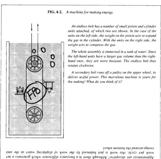
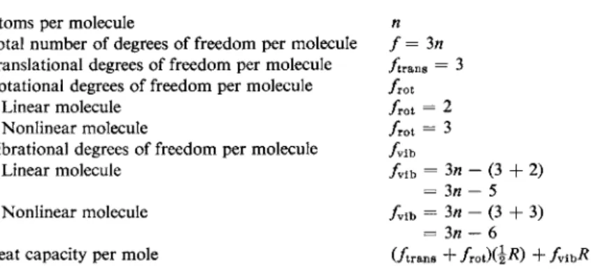
FIG. 4-2. Λ machine for making energy.

An endless belt has a number of small piston and cylinder units attached, of which two are shown. In the case of the units on the left side, the weight on the piston acts to expand the gas in the cylinder. With the units on the right side, the weight acts to compress the gas.

The whole assembly is immersed in a tank of water. Since the left-hand units have a larger gas volume than the right- hand ones, they are more buoyant. The endless belt thus rotates clockwise.

A secondary belt runs off a pulley on the upper wheel, to deliver useful power. This marvelous machine is yours for the making! What do you think of it?

jddUM wojjoq 9 ψ punojv SSUIMS jmn θ ψ SO SuiJOjdsip fo ψ Ο Μ 9 ψ Kq pdouujvq fsnf si ψ ο Μ siu? 'djo^o A d d ψΟΜ.

Idu Ό SdjvjdUdiï UOJUM douajdffip fouvrfonq Ό s i 9Λ9ψ ySnoi/ηγ jdApdaodp ΘΛΌ sdoumOdddy

it is entirely contrary to experience that net heat or work can be put into or with­

drawn from a system without some change in that system. The particular possibility of net work or heat being supplied by a system was for a while intensively tested by attempts to contruct a perpetual motion machine, that is, by attempts to find some cyclic process that produced overall work or heat. The reverse of being able endlessly to insert work or heat into a system without changing it, while less appealing to the inventor, has never been observed either. (Is the device of Fig. 4-2 an exception ?)

We generalize our inability to find a perpetual motion machine by saying that qioi = wtot for any cyclic process. Δ Ε must also always be zero for any such process since the cycle returns the system to the identical state variables of the initial condition; we cannot imagine identical states as having different energies. We thus conclude that ΔΕ is completely defined by Eq. (4-2) and, further, that ΔΕ must be zero for any process for which q = w. In terms of the example here, this means that ΔΕΑΒ must be zero (since qAB = wAB). We also conclude that ΔΕ0Α = —ΔΕΒ€ , irrespective of the nature of state C. Alternatively put, our experience requires that energy changes as defined by Eq. (4-2) be entirely specified when the initial and final states of the process, cyclic or otherwise, are specified. Thus the defining equation (4-2) is not really restricting; it affirms a law of nature of great generality.

4-4 STATE FUNCTIONS. EXACT DIFFERENTIALS 107

The defining equation gives only an energy difference, however; it provides no absolute scale of energy. Ordinarily we pick some standard or reference state as having an assumed energy, usually zero, and then obtain the energy of all other states through Eq. (4-2). In this sense, then, we speak of energy as a state function;

we mean that changes in it are defined if the change of state is defined.

The various preceding statements are ways of affirming the First Law of Thermo­

dynamics. To summarize, the alternative statements are:

ΔΕ

=

The internal energy of an isolated system is constant. (

The internal energy change in a cyclic process is zero.

Internal energy is a state function.

The expression "internal energy" is the correct one for E; it emphasizes that we are referring to the energy content of a definite portion of matter. When indicated by a capital Ε internal energy will be on a molar basis.+

Returning to the example of Fig. 4-1, we see that the requirement to satisfy our experience with respect to perpetual motion machines is that #tot = wtot. Thus, per cycle, it would be allowable for work to be done on the system and an equiv­

alent amount of heat evolved. It would also be allowable for heat to be absorbed and an equivalent amount of work to be done. The first situation encounters no objections, but the second turns out to have a restriction, again as a result of experience. The restriction is stated by the Second Law of Thermodynamics, taken up in Chapter 6.

As a final comment, the first law has so far been justified in terms of negative arguments, that is, in terms of the lack of observations of certain behavior. There is a similar aspect to the second law. However, both lead to relationships that have abundantly been verified. There is thus a great amount of direct evidence for the validity of the laws of thermodynamics.

4-4 Mathematical Properties of State

Functions. Exact and Path-Dependent Differentials

The conclusion that the internal energy change is zero fora cyclic process or that Ε is a state function carries a further implication. Referring once again to Fig. 4-1, we see that the change in energy on going from A directly to Β, ΔΕΑΒ , must be the same as that on going from A to C and then from C to B, AEACB . Otherwise, the first law of thermodynamics would be violated. We conclude therefore that Δ Ε cannot depend on the path taken or that, for some small change, dE is independent of path.

We know, however, that q and w do depend on path. This is a matter of common experience, examples of which are illustrated in Fig. 4-3 and as follows.

CASE 1 State A: mass m at height h.

State B: mass m at h = 0.

Path 1: The object is dropped in free fall and gains kinetic energy mgh, which is dissipated as heat when it strikes the stop at h = 0. No work is done, and so w = 0, but q = —mgh. Thus ΔΕ = q — w = —mgh.

+ We will use ordinary capital letters to denote quantities per mole, sans serif capitals for quantities for an arbitrary amount of system, and small capitals for quantities per molecule, thus : Ε (energy), Ε (energy per mole), and Ε (energy per molecule).

Case 1 State A

State Β

Path 1 Path 2

ο

AE = -mgh

q = -mgh A Ε = -mgh

w = mgh q = 0 A Ε = -mgh

Case 2 Path 1 Path 2

V/////////A State A

γ//////////////////γ

\7/////////////////Λ

State Β

V/////////////////M

0 ΔΕ

= \PdV AE + w FIG. 4 - 3 . Reversible and irreversible processes.

Path 2: The object is counterbalanced by a very slightly lesser mass, which is then raised from h — 0 to h. The work done is now w = mgh, and q = 0, as no significant kinetic energy is developed. ΔΕ = q — w = —mgh.

CASE 2 Stete Gas at Tl9Pl9 and Kx. State 5: Gas at Tl9 P2, and K2.

Pa/A i: The expansion is allowed to occur by rupture of a diaphragm, temperature being kept constant by means of a thermostat bath. No work is done, w = 0, q = ^.E.

Path 2: The expansion occurs against a piston. The work done is (force on piston) χ (dis­

placement) or w = I f dx = J Ps/dx, where is the area of the piston. Hence h> > 0, q = ΔΕ + w.

Thus one of the very important corollaries of the first law is that while Δ Ε depends only on the initial and final states, it is given experimentally by the difference between two quantities q and w which separately do depend on the path taken in going from the initial to the final state. As will be seen in the ensuing material we take advantage of this situation by choosing paths of convenience between two states to facilitate calculation of q and w, knowing that the resulting Δ Ε will be independent of our choice of path. In differential form Eq. (4-2) becomes

dE = Sq - 8w, (4-6) where the deltas are used to emphasize that the path must be specified for q and w.

There is a mathematical parallel which can be developed as follows. First, the state of a system is defined by any two of the state variables V9 P, and T. That is, if we know two of these, the equation of state (for example, the ideal gas law) gives the third. Since Ε depends only on the state, it follows that Ε is some function of any two of the state variables, and as a matter both of convention and of con-

4-4 STATE FUNCTIONS. EXACT DIFFERENTIALS 109

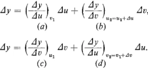
venience we pick V and Τ and write Ε =f(V, T). (For the present it is assumed that no chemical changes can occur; otherwise chemical composition would also have to be specified.) The general mathematical situation is that of a dependent variable y which is some function of variables u and v, y = f(u, v).

A schematic representation of a surface given by y = f(u, v) is shown in Fig.

4-4a. We can define two slopes : (dy\du\ and (dy/dv)u , where the partial differential sign d signifies that the subscript variable is held constant. As shown in the figure, these slopes are those of lines of constant ν and constant u, respectively. Now suppose we wish to go from a point y± to a point y2. Two possible paths would be that marked ab and that marked cd. Accordingly, Ay can be expressed in two ways :

\ Au !Vl \ Av >U2=Ul+Au (a) (b)

Ay=(4-\ Av+(4f-) Au.

\ Av lUl \ Au !V 2 = V l + Av (c) (d)

In the limit of very small differences, Ay = dy, and (Ay/Au)Vi = (Ay/Au)Vi+Av = (dy/8ù)v . A simila r relatio n exist s fo r th e othe r slope . Th e resultin g mathematica l statement i s

and th e correspondin g on e fo r Ε is

(4-8)

FIG. 4-4a. Surface illustrating total and partial differentials.

If dy is integrated between y1 and some value y2, the integral is simply y3 — y1, and, of course, is independent of the path. However, the integrals J^3 (dyldu)v du and (dy/dv)u dv are path dependent. By way of illustration, let y = w r2, so that

dy = v2 du

+

dy = y2 - yi = 36 - 2 = 34,

and this result must be independent of the integration path. Two possible paths are as follows.

Path 1:

(a) (2, 1) to (4, 1):

φ)

Sum : 2 + 32 = 34.

Path 2:

(c) (2, 1) to (2, 3):

(d) (2, 3) to (4, 3):

Sum: 16 + 18 - 34.

v2 j du - ( l )2 (4 - 2) = 2;

2u j ν dv = 8[(32/2) - (l2/2)] = 32;

2u j ν dv = 4[(32/2) - (l2/2)] = 16;

v2

j

(4,3)

FIG. 4-4b. The function y = uv2^.

4-4 STATE FUNCTIONS. EXACT DIFFERENTIALS 111

Thus although the two integrals v2 J du and 2u j ν dv depend on path, their sum does not.

The differential dy in Eq. (4-7) is known as an exact differential; its integral is independent of path. However, this is not necessarily true of every expression of the form

dy = Mdu + Ndv. (4-10) For example, the expression (v du + 2uv dv) is not an exact differential. It

is possible to test an expression such as Eq. (4-10) on this point. Referring to Eq. (4-7), for an exact differential, we have

ldM\ _ / d2y \ / dN \ _ / d2y \

\ dv ) u \ du dv 1 9 \ du Jv \ dv du /

Most thermodynamic functions are continuous and single-valued, so the order of partial differentiation makes no difference. It follows that

(dM\ i dN \ , . i n

t )

= b d ;

"

The expression (v2 du + 2uv dv) meets the test of Eq. (4- l l ) whereas (v du + 2uv dv) does not.

Where the differential is known to be exact Eq. (4-11) is very useful in providing an additional relationship. Such a relationship is known as an Euler or a cross- differentiation equation and will occur fairly often in Chapter 6.

Mathematics provides two additional very useful equations. Since u and ν are independent variables du and dv may be chosen independently. In particular they may be chosen so that dy = 0. Equation (4-7) then becomes

or expressing the constancy of y in the equation,

\dvly (ôy/du)v

Thus

,_eV\ = _ (8E/8T)V

\dT)E (8E/8V)T- yH lJ>

A specific example may help at this point. Let V = f(P, T). Then

If the gas is ideal, (dV/dP)T = -RT/P2 and (dV/8T)P = R/P; by Eq. (4-12), (dP/dT)v is given by

dP \ (dV/dT)P RIP Ρ

( θτ)

The derivative (dP/dT)v may be found directly. Thus Ρ = RT/V, so (3P/dT)v = R/V = P/T.

The result is the same as by the indirect method.

Second, if there is some quantity ζ which is a function of u and v, then one can impose the condition on du and dv that ζ be constant:

This constancy is usually indicated in partial differential form by dividing through by duz or by dvz ; thus

&).-(£).(£).-<-(&).· <«»

For example, since Ρ = / ( K , Γ), on applying the condition of Ρ constant to Eq. (4-8), we obtain

/ dE \ ι dE \ ι 3V \ ι BE \ ίλ Λ„

Μ ^ ( τ γ )

( ^ 1

( - ^ ) , ·

-

4-5 Heat and Work for Various Processes

A. Evaluation of η; Heat Capacity

As emphasized earlier, the value of q for a change of state depends on the path, so the path must always be specified. There is, of course, an infinite number of possible types of paths that a system might follow in going from one state to another, but we find it very convenient, both experimentally and theoretically, to emphasize a few special ones. We thus make much use of the following types of process.

(1) Adiabatic. q = 0. The system is insulated so that no heat can enter or leave.

(2) Isochoric. The system is constrained to a definite volume. We introduce the coefficient (dq/3T)v or, as a convenient nomenclature, specify the path by writing qv , and hence dqv\dT. This type of coefficient is called a heat capacity (the term specific heat refers to heat capacity relative to that of the same mass of water) C. For a constant-volume path C becomes Cv :

r _ dqv

Further, under constant-volume conditions no mechanical work w can be done.

As a consequence ΔΕ = qv , or dEvjdT = Cv . Alternatively, by Eq. (4-8) we can write

(4-17) (3) Isobaric. The system is maintained at a particular pressure during the process. Following the preceding formalism we have

, _ dqP

P~ dT' (4-18)

4-5 HEAT AND WORK FOR VARIOUS PROCESSES 113

β . Evaluation of w; Reversible Work

We will not ordinarily consider situations such as case 1 of Fig. 4-3, involving work in a gravitational field, nor, for the present, situations involving chemical work. However, a number of very useful results in chemical thermodynamics follow from treatments of mechanical or pressure-volume work. As noted in Section 4-4, mechanical work occurs if a system is compressed or is allowed to expand. Although it is helpful to visualize a gas, the following discussion applies to any type of substance. As illustrated in Fig. 4-5, we imagine the substance to be contained in a piston and cylinder arrangement. There is an external pressure Pe xt on the piston and the force on the piston is then Pextsi, where si is its area. Since work is given by / dx9 we can write

w = j f dx = j Pext-si dx.

However, si dx is just the volume change, so a more useful form is

W = / Pext dV. (4-19)

At this point an important practical consideration enters. We want w as defined in connection with Eq. (4-2), that is, the work done by the system on its surroun­

dings, or by the surroundings on the system. Thus the pressure in Eq. (4-19) must be the pressure felt by the piston, that is, the external pressure Pex t . However, while

t ~ i Fixed stop

k—δχ- (a)

Movable stop

F I G . 4 - 5 . Reversible (a) and irreversible (b) expansions, (c) Illustration of Eq. (4-20).

the value of Pext would be important in obtaining the work output of a machine, it is not directly significant to the thermodynamics of the fluid. For example, the cylinder might contain a gas at 1 atm pressure confined by a piston held in place by means of a stop as shown in Fig. 4-5(b). The pressure Pe xt is defined by some weight W placed on the piston. The weight W might be such as to make pe xt = 0.1 atm. The stop is pulled out and the piston moves back to the second stop, thereby increasing the volume. The work done is 0.1 Δ V, in liter atmosphere.

Were W such as to make Pext = 0.2 atm, then w would have been 0.2 Δ V, and so on.+ Thus w could have any value from zero (W = 0) up to some maximum value.

What we are interested in is this maximum value.

Clearly, the maximum possible value of w would be obtained if Pe xt (or W in the figure) were steadily adjusted so as always to be only slightly, or, in the limit, infinitesimally less than the pressure of the gas, which is the pressure P. Not only do we now have the maximum work, but since Pext = P , we now know how Pe xt must vary with the volume. That is, the equation of state of the substance gives us Ρ as a function of Γ and V, Ρ = f(T, K), so Eq. (4-19) becomes

H W = j Ρ dV = j f(T, V) dV, (4-20) [note Fig. 4-5(c)].

We speak of the condition of Pe xt = Ρ as giving the reversible work. Thus from Fig. 4-5(a) if Pe xt is slightly less than P , expansion occurs, while if Pe xt is made slightly more than P , compression occurs. Thus the direction of the process can be reversed by an infinitesimal change in Pe xt. Reversible processes will be of central importance in the development of chemical thermodynamics, since by means of them we can calculate w if we know the equation of state of the substance and since they give the limiting or maximum value of w.

We may next consider w in terms of the various standard processes.

(1) Adiabatic q = 0. We do not know w directly, but, by the first law, it follows that

dE = -8w = -PdV. (4-21) (2) Isochoric w = 0. This follows since dV = 0, as noted previously. Then

dE = Cv dT. (4-22)

(3) Isobaric w = ΡΔν. Since pressure is constant, it may be put in front of the integral of Eq. (4-20). Also,

dE = CPdT - Ρ dV. (4-23)

Where only reversible mechanical work is involved, the first law evidently can be written in the form

dE = 8q — Ρ dV. (4-24) The various special cases then follow from Eq. (4-24). It should be emphasized that

whenever Ρ rather than Pe xt is used, the process must be a reversible one.

+ We can suppose that in each case friction prevents the piston and weight from gaining kinetic energy and that the frictional heat is dissipated into the gas. [See D. Kivelson and I. Oppenheim, / . Chem. Ed. 43, 273 (1966) for a discussion of this type of experiment.]

4-6 ENTHALPY. AN ALTERNATIVE FORM OF THE FIRST LAW 115

4-6 Enthalpy. An Alternative Form of the First Law

The first law takes on a particularly simple form for an isochoric process, in that dE is simply Cv dT. Actual experiments are more often done under constant- pressure conditions, and the following alternative statement of the first law is very useful. We define a new molar quantity H called the enthalpy:

H = E+ PV. (4-25) Since the volume and pressure of a system are determined solely by its state, as is E,

H must also be a state function. The differential form of Eq. (4-25) is

dH = dE + PdV + VdP (4-26) and, using Eq. (4-24), we have

dH = 8q + VdP. (4-27) We then have the following special cases, corresponding to the standard

processes.

(1) Adiabatic Since q = 0, it follows that

dH = VdP. (4-28) (2) Isochoric

dH = CvdT+ V dP. (4-29)

(3) Isobaric Since dP is zero,

dH = CP dT [or (^γ) = CP] . (4-30)

Since H is a state function, its value depends on those of the state variables, Ρ, V, and Γ, any one of which can be eliminated by means of the equation of state of the system. In the case of E, it is natural to pick V and Τ as the independent variables; in the case of H, the natural choices are Ρ and T. Since dH is an exact differential, we have

+(4r),

- <«•>

and

( dT )„ (dH/8P)T ' ^ ό Ζ)

The introduction of the enthalpy function allows the following derivation of an important relationship for the difference between CP and Cv :

or, from the definition of H, Eq. (4-25),

This equation is discussed further in the Commentary and Notes section.

4-7 Applications of the First Law to Ideal Gases

A. Internal Energy Change for an Ideal Gas

The application of the first law to the case of an ideal gas not only provides simple illustrations of its use but turns out to be of considerable importance generally. To anticipate a little, the reason for this last statement is that ideal gas behavior is the limiting behavior of all real gases, so that the results are not hypothetical but provide the reference condition for treating nonideal behavior.

Further, any solid or liquid is in principle in equilibrium with its vapor; knowledge of the thermodynamic properties of the vapor may therefore be used as an indirect path to treatment of the solid or liquid state. Finally, most gases are approximately ideal, so the thermodynamics of the ideal gas is often used directly to give approx­

imate results, usually of acceptable accuracy, for real gases and vapors at ordinary pressures.

We owe again to Joule a fundamental piece of information—this time about an ideal gas. His experiment, described in 1843 and illustrated in Fig. 4-6, consisted of allowing air under pressure (up to 10 or 20 atm) to expand from one vessel into another. There was no change in the temperature of the gas. Alternatively, the two (4-34)

#0 ^{c h}

F I G . 4 - 6 .

Joule's

On eliminating (dE/dT)P by means of Eq. (4-16), we obtain as the final result

4-7 APPLICATIONS OF THE FIRST LAW TO IDEAL GASES 117

bulbs were immersed in a water bath; no change in the temperature of the bath could be observed when the expansion occurred. The significance of this result is that since no work was done, w = 0, and since no temperature change occurred, q = 0; therefore Δ Ε was zero.

More accurate later experiments have shown that Joule's experiment does in fact lead to small temperature changes (see Special Topics) but that in the limit of ideal gas behavior, his conclusion was correct. The conclusion, in partial differential form, is

(W)E = 0 ⁽i ^sda^{) - (}es a l 4^"3⁾ 5 (Equations valid specifically for an ideal gas will be so labeled.) It follows from

Eq. (4-13) that

( - | | - ) = 0 (ideal gas) (4-36) and, from Eq. (4-8), that

dE = (-||-) dT (ideal gas) dE or

§ = ( W ) r

-

-

This last, very important result says that for an ideal gas the change in energy with temperature is always given by CvdT, regardless of the actual path; that is, regardless of whether V is constant or not.

A similar situation holds for enthalpy. It follows from the defining equation for Η that

3H_\ _ i_dE_\ , (d(PV)\

\3P ) T V 0P /r \ W

V

The last term is zero for an ideal gas; also

/ dE \ _ l^E_\ / dV \

\ dP J τ ~ \ dV ) T \ dP ) T

(a partial derivative may be expanded in this manner if the same quantity is held constant in all terms), and since (3E/dV)T is zero, it follows that

( - ! ! - ) = 0 (ideal gas). (4-38) The result is therefore that

Then, from Eqs. (4-31) and (4-30), dH ι dH

§ = ( ^ ) =

-

"

>

Thus for an ideal gas the change in enthalpy with temperature is always given by CP dT, regardless of the actual path.

We can also relate CP and Cv . By Eq. (4-34), CP - Cy = (P + 0) y

or

CP- Cv = R (ideal gas). (4-41)

6 . Various Processes for an Ideal Gas

The various quantities are as follows for the indicated type of reversible process.

Isochoric

w = 0,

dE = CvdT^ dqv [Eq. (4-22)],

dE = Cp dT [ideal gas, Eq. (4-40)].

Isobaric

dw = PdV= RdT, w = RAT (ideal gas), (4-42) dE = Cv dT [ideal gas, Eq. (4-37)],

dE = CPdT= dqP [Eq. (4-30)].

The isothermal or constant-temperature process was not considered in Section 4-5 since it leads to no specialized forms in the general case. However, for an ideal gas if dT is zero, then dE = 0 and dE = 0. It follows that q = w, and w = ρ dV = (RT/V) dV = RTd{\n V). Since at constant temperature

In V + In Ρ = constant, d(\n V) = — έ/(1η Ρ) and w = ~RTd(\n P).

In summary we have the following results.

Isothermal

q = w,

dw = RTd(\n V) =—RTd(ln P) (ideal gas), (4-43) or

w = RT In - RT In A. (ideal gas), (4-44)

</£ = 0, dE = 0.

Finally, for an adiabatic process, q is zero and since, for an ideal gas, dE is always Cv dT, Eq. (4-21) can be written

or

Cv dT = -PdV= —RTdQn V)

Cv d{\n T) = -R d(ln V) (ideal gas). (4-45) Alternatively, d(\n Ρ) + ί/(1η V) — d(ln T) for an ideal gas, so, on eliminating

ί/(1η V) and remembering that CP = CV + ^ , we get

CP rf(ln 7 ) = i? rf(ln P ) (ideal gas). (4-46) If the heat capacities are independent of temperature (as discussed later) then the

equations may be integrated directly. In summary we have the following results.

Adiabatic

dq = 0, dw = —dE,

dE = Cv dT [ideal gas, Eq. (4-37)], dE = CP dT [ideal gas, Eq. (4-40)],

4-7 APPLICATIONS OF THE FIRST LAW TO IDEAL GASES 119

[ideal gas, Eq. (4-45)], [ideal gas, Eq. (4-46)],

(ideal gas), (4-47) (ideal gas), (4-48) (ideal gas). (4-49) The last form is obtained as follows. Equation (4-47) may be written as

(Γί/ΓΟ = {VJVJ*'cv - (Vi/V2y-\ Since (TJTJ = (P2V2/P1V1), elimination gives (PJPi) = ( ^ i / ^2)y or PXV^ = P2V2V. Equation (4-49) is a generalization of this last conclusion.

C. Heat Capacity of an Ideal Gas

This subject is treated in more detail in Section 4-8. For the present, it is useful to consider qualitatively a special case of the general heat capacity behavior for an ideal gas. The special case is that of an ideal, monatomic gas. Such a gas can have only kinetic energy; its molar internal energy is then, from Eq. (2-4),

Ε = %RT.

The heat capacity of the gas is therefore

Cv = | P (ideal monatomic gas) (4-50) and CP , of course, is (Cv + R), or

CP = %R (ideal monatomic gas). (4-51)

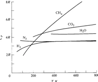
Gases, even though ideal, will in general have a higher heat capacity than that given here. If the molecule has more than one atom, then as the temperature is raised energy goes into vibration and rotation as well as into increased kinetic energy. The degree to which this happens increases with increasing temperature;

some typical heat capacity curves are given in Fig. 4-7. It is convenient for many calculational purposes to represent this temperature variation by means of a poly­

nomial in temperature:

CP = a + bT + cT~2 + ··· (4-52)

and some values for such coefficients are given in Section 5-6.

D . Some Calculations for an Ideal, Monatomic Gas

A number of equations have been introduced in this section for processes involving an ideal gas. The following example is intended to illustrate their appli-

Cvd(\n T)= -Rd(\n V) CP d(\n T) = R d{\n P) and, if Cv and hence also CP are constant,

C Fl n ^ = Ρ ΐ η ψ PVy = constant, γ =

200 400 600 800 Τ, Κ

FIG. 4-7. Heat capacity CP as a function of temperature for various gases.

cation in a way that will also bring out important features of the first law of thermodynamics. We will use one mole of an ideal, monatomic gas as the working fluid—we can then use the constant values of Cv and CP of %R and %R, respectively, and thus simplify the calculations.

The gas initially is in state 1 at 0°C and 10 atm pressure, and hence at 2.241 liter volume. It is put through the following reversible cycle, cycle A in Fig. 4-8.

State 1 (273K)

State 3 (27.3K) State 2' (108.7K) State 2 (273K) I ι I ι ι ι I 2.24 8.92 10 20 22.4

V, liter

FIG. 4-8. Two reversible ideal gas cycles (see text).

4-7 APPLICATIONS OF THE FIRST LAW TO IDEAL GASES 121

TABLE 4 - 1 . Calculations for the Two Cycles of Fig. 4-8a

Change of state Process Q w ΔΕ ΔΗ

Cycle A

1 to 2 Isothermal 629.0 629.0 0 0

2 to 3 Isobaric - 6 1 4 . 5 - 2 4 5 . 8 - 3 6 8 . 8 - 6 1 4 . 6

3 to 1 Isochoric 368.8 0 368.8 6Γ4.6

Cycle 383.3 383.3 0 0

Cycle Β

1 to 2' Adiabatic 0 246.6 -246.6 - 4 1 1 . 0

2' to 3 Isobaric -203.5 - 8 1 . 4 -122.1 -203.5

3 to 1 Isochoric 368.7 0 368.7 614.5

Cycle 165.2 165.2 0 0

°A11 values in terms of R(K).

State 1 to state 2: Isothermal expansion to 1 atm. Then V2 = 22.41 liter, T2 = 273.15 K,

w = RT In ξ-1 = *(273.15)(2.303)(1) = 629.0*, q = w = 629.0*, ΔΕ = ΔΗ = 0.

The results can all be expressed in units of ( * ) ( K ) ; we can obtain the actual values in calories by putting R = 1.987 cal K "1 m o l e "1, or in joules by using R = 8.314 J K "1 m o l e '1.

State 2 to state 3 : Isobaric cooling to 2.24 liter. Then T3 =ζ?Τ2= 27.315 Κ, Ρ , = 1 atm,

w = RAT= *(27.32 - 273.15) = - 2 4 5 . 8 * , q = CPAT = f* ( - 2 4 5 . 8 ) = - 6 1 4 . 5 * , ΔΕ =CVAT = f* ( - 2 4 5 . 8 ) = - 3 6 8 . 8 * , ΔΗ = CPAT = q = - 6 1 4 . 6 * .

State 3 back ίο state 1 : Isochoric heating to 273.15 Κ, 10 atm, and 2.241 liter.

Then

w=0, q = CVAT = f*(273.15 - 27.32) = 368.8*, ΔΕ = q = 368.8*, ΔΗ =CPAT = 614.6*.

The results for cycle A are summarized in the top part of Table 4-1. Notice that for the cycle q = w and ΔΕ and ΔΗ are zero. A further point is that since w = j Ρ dV, if a path is plotted as * versus V, then w is given by the area under that path. The area is positive for a left-to-right direction of progress along the path and negative for a right-to-left one. As a result the total work associated with a closed path or cycle is just the area enclosed by the cycle.

Next consider a second reversible cycle Β using the same starting point; this is also shown in Fig. 4-8. The steps are now as follows.

.74) = - 8 1 .4 R , -- -203.57?,

= -122.17?,

4-8 Molecular Basis for Heat Capacities. The Equipartition Principle

It was pointed out in the preceding section that since the internal energy for an ideal monatomic gas consists only of its kinetic energy, Cv is therefore f 7?.

Also, in Section 2-CN-l, it was noted that the heat capacity for a one- and a two-dimensional gas is Cv = |7? and 7?, respectively. Thus each independent velocity component has associated with it a molar kinetic energy of \RT and corresponding heat capacity of Cv = |7?. These three independent modes of translation in three dimensions reflect the fact that three coordinates are needed

State 1 to state 2': Adiabatic expansion to 1 atm. Then l o g ^ ' / ^ ) = (2/5) l o g ( / V / i \ ) = - 0 . 4 0 0 or Tr = 0.39817\ = 108.74 Κ. Then

Vv = (108.7/273.15)(10/1)(2.241) = 8.92 liter.

Further,

q = 0,

AE = CVAT = f7?(108.74 - 273.15) - - 2 4 6 . 6 / ? , w = -ΔΕ = 246.67?,

ΔΗ = CP ΔΤ = |7?(108.7 - 273.15) = -411.07?.

State 2' to state 3 : Isobaric cooling to 2.24 liter; Tz = 27.31 Κ and Ps = 1 atm, as before. Then

w = RAT = 7?(27.32 - 108 q = CP AT = f7?(-81.4) = ΔΕ = Cv ΔΤ = |7?(-81.4) = ΔΗ = q = -203.5/?.

State 3 back to state 1 : Same as for cycle A.

This second set of results is assembled in the bottom part of Table 4-1. Again Δ Ε and ΔΗ are zero for the cycle, but notice in Fig. 4-8 that the P-V plot of the adiabatic expansion 1 -> 2' is steeper than that of the isothermal one 1 —> 2. The physical reason for this is that in the adiabatic expansion the energy for the work done is supplied by a cooling of the gas. The temperature thus drops steadily during the expansion and the volume at each stage is less than at the corresponding pressure during the isothermal expansion. As a result the area under the Ρ- V plot for the adiabatic process is smaller than that under the one for the isothermal process, and this is in conformity with the lesser amount of work done. The further consequence is that less work is done by cycle Β than by cycle A, and a corre­

spondingly smaller amount of heat is absorbed.

Notice also that while q and w are different for the sequences 1 -> 2 —• 3 and 1 - > 2 ' -> 3, the values of ΔΕ and AH are the same. We thus have a further illustration of the point that q and w are dependent on the path taken between two states, but Δ Ε and AH are not.

4-8 MOLECULAR BASIS FOR HEAT CAPACITIES. THE EQUIPARTITION PRINCIPLE 123

FIG. 4 - 9 .

to specify the position of a particle in space and, by means of their time derivatives, the velocity of a particle in space.

We speak of the number of degrees of freedom / of a system as the number of variables that must be specified to fix the position of each particle or the velocity of each particle. For one mole of particles there are 3N0 degrees of freedom.

Consider next the case of an ideal gas composed of diatomic molecules. There are now two moles of atoms and so, per mole of molecules, / = 6N0 . To generalize, a gas consisting of η atoms per molecule will have 3nN0 degrees of freedom per mole, orf=3n per molecule.

Returning to the case of the gas consisting of diatomic molecules, although one could specify the positions of all atoms by means of 6NQ coordinates per mole, there is a more rational and very useful alternative scheme. One recognizes that the gas in fact consists of molecular units of two atoms each. Of the six degrees of freedom required to locate two atoms, one first uses three to locate the center of mass of the molecule. One now needs to specify the positions of the two atoms relative to their center of mass. As illustrated in Fig. 4-9 two angles will be needed or, alternatively, the degrees of rotation around the χ axis and around the y axis.

Rotation about the molecular or ζ axis does not change the nuclear positions and hence contributes no information. (In the case of a nonlinear molecule, however, all three rotations would be needed.) If now we also specify the distance between the atoms, the description of their position in space is completely fixed. Thus six coordinates are also needed in the alternative scheme. In general, the number of coordinates sufficient to describe the positions of a set of η atoms cannot depend on the scheme used but is always equal to the 3n degrees of freedom.

As just noted each degree of translational freedom implies an energy of ^RTper mole and a heat capacity contribution of | * per mole. In the alternative scheme of describing the positions and velocities of atoms the rotational degrees of freedom must likewise contribute %R each to Cv. It might be supposed that the same should be true for those degrees of freedom describing interatomic distances.

Here, however, a new factor enters. The atoms of a molecule are held together by the attractive forces of chemical binding. They execute vibrations, rather than simple motions, and their interatomic distances are therefore some periodic function of time. Thus in the case of the diatomic molecule of Fig. 4-9, drjdt is also a function of time. It is zero at the end of a vibrational stretch or compression

and a maximum in between; consequently drjdt is insufficient to specify the total energy of the vibration, and one needs to state the potential energy as well as the kinetic energy for each value of r.

The conclusion from this analysis is that each vibrational degree of freedom should contribute twice the usual amount to the heat capacity, or that the total heat capacity associated with vibrations should be Rfvix>, wherefVi\> denotes the number of vibrational degrees of freedom. This same conclusion is obtained in Section 4-12 as a result of a quantum statistical mechanical treatment.

In summary, we have the following results.

Atoms per molecule

Total number of degrees of freedom per molecule Translational degrees of freedom per molecule Rotational degrees of freedom per molecule

Linear molecule Nonlinear molecule

Vibrational degrees of freedom per molecule Linear molecule

Nonlinear molecule Heat capacity per mole

η f = 3«

/trans = 3 /rot /rot = 2

/rot = 3 fwib

/v lb = 3n - (3 + 2)

= 3n- 5 /v ib = 3n - (3 + 3)

= 3Λ — 6

(/trans +/rotX^) + fvihP Some representative applications are given in Table 4-2.

This treatment of heat capacity is based on two principal assumptions. The first is that potential energy contributions are present only for vibrations within the molecules and not for those between molecules. The gas is therefore assumed to be ideal. The second assumption is that each degree of freedom has associated with it a heat capacity contribution of %R (or R9 if a vibration). The principle which states this assumption is known as the principle of the equipartition of energy. It is a principle based on classical mechanics and, as will be seen in Sections 4-11 and 4-12, it can be in serious error. A glance at Fig. 4-7 shows that, at best, the equipartition values of heat capacities are only approached at high temperatures.

A closer look suggests that for molecules around room temperature the equi­

partition contributions from translation and rotation have been reached and that the main discrepancy lies with the vibrational contribution. An important function

TABLE 4 - 2 . Applications of the Equipartition Principle

Molecule / /trans /rot /vib

Equipartition heat capacity per mole in units of R

Cv Cp

Ar 3 3 0 0 3/2 5/2

N2 6 3 2 1 7/2 9/2

C 02 ^{(linear) 9 3 2 4 13/2 15/2}

H20 (nonlinear) 9 3 3 3 12/2 14/2

CH4 ^{15 3 3 9 24/2 26/2}

Monatomic 3 0 0 3 6/2 - 6 / 2

crystalline solid

MX type of 6 0 0 6 12/2 —12/2

crystalline solid

4-9 STATISTICA L MECHANICA L TREATMEN T O F FIRS T LA W QUANTITIE S 12 5

of th e statistica l mechanica l treatment s tha t follo w i s th e providin g o f a detaile d explanation o f ho w an d wh y hea t capacitie s var y a s the y d o wit h temperature .

4-9 Statistica l Mechanica l Treatment o f Firs t La w Quantitie s

A. The Partition Function. The Average Energy per Molecule

It i s sufficien t fo r th e presen t t o regar d a syste m a s bein g mad e u p o f non - interacting molecule s eac h o f whic h ha s variou s translational , rotational , an d vibrational energ y states . Accordin g t o th e Boltzman n principl e (Sectio n 2-2) , th e probability o f a molecul e bein g i n som e energ y stat e e{ i s proportiona l t o e~€i/kT. It i s no w ver y usefu l t o writ e th e su m ove r al l suc h energ y state s an d t o giv e thi s sum th e specia l nam e o f partition function Q :

Q =

Z^-

.

i

The facto r g{ i s a weightin g facto r allowin g fo r th e possibilit y tha t certai n inde - pendent configuration s hav e identica l energies . Suc h a situatio n i s calle d a degene- racy; tha t is , i f a molecul e ca n hav e a n energ y e{ i n mor e tha n on e way , tha t energy stat e i s sai d t o b e degenerate.

We ca n no w writ e a n expressio n fo r th e averag e energ y o f a molecule , followin g the usua l averagin g procedure , give n b y Eq . (2-34) :

It i s a n assumptio n i n statistica l mechanics , th e rigorou s defens e o f whic h wil l no t be give n here , tha t th e averag e energ y ë whic h a particula r molecul e shoul d hav e i s also th e averag e energ y pe r molecul e i n a larg e collectio n o f molecules , E . N O W, fro m Eq. (4-53) , dQ/dT = Σζ (*i/kT2) g ^ ^ 7; consequently Eq. (4-54) can be written in the form

E = kd ^ TT =2 k^ Q lT ( 42 .5 5)

or, per mole,

ai

Equation (4-56) may be written in the form E~ " ' d(\/T)

since (—l/T2)dT=d(\/T) (as noted in Section 1-7). The expression for ë [Eq. (4-54)] is for the average molecular energy, and its temperature dependence does not include any pressure-volume work, so that constancy of volume, implicit in the equation, is now stated explicitly.

Since Cv = (dE/dT)v = -T-2[dE/d(l/T)]v, we obtain from Eq. (4-57)

R ra2(lnQ) ι u

Enthalpy may also be expressed in terms of the partition function,

Η = Β + P v = kl- [ i ^ ] y + *7V [ i ^ ] r ; H = NQÎI. (4-59) The derivation is best made using the second law of thermodynamics, however, and is therefore postponed until Section 6-9.

β . Separation of the Partition Function into Translational, Rotational, and Vibrational Parts

The energy e{ of the ith state of a molecule will in general consist of the sum of the translational, rotational, and vibrational energies. In addition, if the state is one of electronic excitation, then this is added, too. As is discussed in the material immediately following, each type of energy is quantized. A molecule thus might be in the nth translational energy level, in the tenth rotational level, and in the second vibrational level, as a specific example. To a good first approximation, however, the energy of, say, the tenth rotational state is independent of what translational or vibrational state the molecule is in. If this approximation is made, a very con­

venient factoring of the partition function becomes possible.

Suppose that just two kinds of energy states are possible, denoted by e£ and e/;

these might, for example, be translational and rotational states. The molecule may then be in state e1, e2, e3, ... with respect to the first kind of energy and at the same time in state e/, e2', e3', ... with respect to the second kind of energy. Possible total energy states would then be + c/), (€l + e2'), (*i + e3')> ·> (€2 + *ι'Χ 02 + e2'),

(€2 + €3,) » ···> (€3 + €i' ) v · The corresponding partition function would then be

Q = g-iCi+c^/kT _J_ E-tet+e^y/kT _|_ . . · - } - E-(£2+€I'VkT + ···

(We may avoid using the weighting factors gz simply by listing each state as many times as it is degenerate.) This equation can be written as

Q = ⁽E^-€^I/T ^{E -}KE^I/ ^{) + (E-}K T€^I/KT ^E~€²,/KT) + ··· + (E~€²/KT^E~€^{^'}LKT^{) + ··· .}

It is now possible to group terms :

Q = E~€^I/KT^(E~€^I/KT ^{+ E~^'}LKT'+ ···) + E-^LKT^{{E-^'}LKT ^{+ E ~ ^}T T ^{+ ···)} , K _|_ e-tzlkT(ç-ex'lkT _|_ e-e2'/kT^_ ·..)-(- ... #

If we make the stated assumption, namely that a given € state has an energy value that is independent of which e state is involved and vice versa, then the sums in parentheses are identical, and the whole expression reduces to the product of two sums. Thus

Q =

(Σ

~

)(Σ

Q = ( Σ ^

*

) ( Σ Λ ' ^ ' '

*

)

i i

4-10 TRANSLATIONAL PARTITION FUNCTION FOR AN IDEAL GAS 127

or

Q = Q Q '

The assumption of the mutual independence of energy states therefore allows the partition function to be expressed as a product of the separate partition functions for each kind of state. We can write

Q = QtransQrotQvibQelec · (4-60) It follows from Eq. (4-56) that

Ε = £trans + EToi + £ y i b + £ e l e c . (4-61) The approximation thus leads to the reasonable conclusion that the total average

energy can be regarded as the sum of the separate average energies of translation, rotation, etc. It further follows from Eq. (4-58) that Cv may also be written as a sum of corresponding contributions:

Cv = CV(trans) + CV(rot) + CV(vib) + CV(elec) · (4-62) The same is true for H.

We will neglect partition functions due to a sum over electronic excited states because the energy of such states is usually so large that they are not populated at ordinary temperatures. We do this by setting Q e i e c equal to unity, on the following basis. If the first and higher electronic excited states are large in energy compared to kT9 then all but the first term in Q e i e c will be negligible, and

Q e l e c = ^ 1 ,

where e± is the energy of the first electronic state. In general, we do not know absolute energy values, only relative ones, and we can set et = 0 as our reference point. However, even if e± were assigned some nonzero value, the consequence would simply be to add this value to e. Thus, referring to Eq. (4-55), we obtain

Eelec = ( ^ ) kT2

Our neglect of Qeiec then amounts, at the most, to regarding the absolute energy of the first electronic state as making a constant contribution to E. We ordinarily do set e1 = 0 for electronic energy, but in the case of vibrational energy, we will use a nonzero value for energy of the first state (see Section 4-12).

4-10 Translational Partition Function for an Ideal Gas

A result from the wave mechanical treatment of a particle in a box, which will not be derived until Section 16-5B, gives the sequence of energy states that corresponds to a particle which is free of any interaction with other particles.

In this respect, the picture is analogous to that used in Section 2-1 for the simple