Using regression tree ensembles to modelinteraction effects: a graphical approach

(1)

Full Terms & Conditions of access and use can be found at

https://www.tandfonline.com/action/journalInformation?journalCode=raec20

Applied Economics

ISSN: 0003-6846 (Print) 1466-4283 (Online) Journal homepage: https://www.tandfonline.com/loi/raec20

Using regression tree ensembles to model interaction effects: a graphical approach

Fritz Schiltz, Chiara Masci, Tommaso Agasisti & Daniel Horn

To cite this article: Fritz Schiltz, Chiara Masci, Tommaso Agasisti & Daniel Horn (2018) Using regression tree ensembles to model interaction effects: a graphical approach, Applied Economics, 50:58, 6341-6354, DOI: 10.1080/00036846.2018.1489520

To link to this article: https://doi.org/10.1080/00036846.2018.1489520

View supplementary material

Published online: 05 Jul 2018. Submit your article to this journal

Article views: 3755 View related articles

View Crossmark data Citing articles: 1 View citing articles

(2)

Using regression tree ensembles to model interaction effects: a graphical approach

Fritz Schiltz ^a, Chiara Masci^b, Tommaso Agasisti^cand Daniel Horn^d

aLeuven Economics of Education Research, University of Leuven, Leuven, Belgium;^bDepartment of Mathematics, Modelling and Scientific Computing, Politecnico di Milano, Italy;^cDepartment of Management, Economics and Industrial Engineering, Politecnico di Milano, Italy;

dCentre for Economic and Regional Studies, Hungarian Academy of Sciences, Hungary

ABSTRACT

Multiplicative interaction terms are widely used in economics to identify heterogeneous effects and to tailor policy recommendations. The execution of these models is often flawed due to specification and interpretation errors. This article introduces regression trees and regression tree ensembles to model and visualize interaction effects. Tree-based methods include interactions by construction and in a nonlinear manner. Visualizing nonlinear interaction effects in a way that can be easily read overcomes common interpretation errors. We apply the proposed approach to two different datasets to illustrate its usefulness.

KEYWORDS heterogeneous effects;

Regression trees; interaction effects; machine learning;

education economics JEL CLASSIFICATION C50; I21

I. Introduction

The estimation of interaction effects has received considerable attention as they are frequently used by economists to identify heterogeneous treatment effects (Ai and Norton, 2003; Karaca-Mandic, Norton, and Dowd 2012). A common approach is to include multiplicative interactions. However, the execution of these models is often flawed due to the lack of conditional hypotheses (specification errors) and interpretation errors (Brambor, Clark, and Golder 2006). A conditional hypothesis such as ‘an increase inX is associated with an increase in Ywhen Z = 1ʹ implies the need for an a priori specification of this interaction effect. If the interaction term is not specified, it will not be estimated in a standard regression approach. In many empirical studies, when interaction effects are added, constitutive terms are not included, biasing the estimation and interpretation of coefficients (Brambor, Clark, and Golder 2006). In addition, interaction effects are generally included linearly (Hainmueller, Mummolo, and Xu 2017).

This article introduces regression trees and regression trees ensembles, rooted in the machine learning (ML) literature, and illustrates how these methods can be useful to model interaction effects.

ML methods are increasingly being used in different fields. Applications include, among others, predict- ing worker productivity (Burns and Köster 2016), poverty alleviation (Blumenstock 2016), classifying economics journal content (Angrist et al. 2017), textual analysis in real estate (Nowak and Smith 2017), and even modelling judges’ jail-or-release decisions (Kleinberg et al.2017). The motivation to use regression trees and ensembles to model interaction effects is threefold. First, tree-based methods include interactions by construction, without requir- ing the researcher to have any preconception on this matter (Su et al.2011). As a result, common specification errors can be overcome. Second, discontin- uous relationships and nonlinear interaction effects are more naturally accommodated by tree-based methods, as opposed to multiplicative interactions.

Third, joint plots visualize interactions between variables, providing applied economists with a useful tool to explore interaction effects in an intuitive way.

We illustrate the approach using two datasets on schools in Hungary and Italy. Our data for Hungary covers the 2008–2010 period and includes variables with respect to all organizational levels in primary education (student, class, school and education provider). Our data for Italy covers the 2013–2016

Supplemental material for this article can be accessedhere.

CONTACTFritz Schiltz fritz.schiltz@kuleuven.be University of Leuven, Naamsestraat 69, Leuven 3000, Belgium https://doi.org/10.1080/00036846.2018.1489520

This is an Open Access article distributed under the terms of the Creative Commons Attribution-NonCommercial-NoDerivatives License (http://creativecommons.org/licenses/by-nc- nd/4.0/), which permits non-commercial re-use, distribution, and reproduction in any medium, provided the original work is properly cited, and is not altered, transformed, or built upon in any way.

(3)

period and contains extensive information on student characteristics (e.g. socio-economic status (SES), immigration). Both datasets allow estimating a value-added (VA) approach since the same students are followed over time. Student achievement can be seen as the outcome of a production process characterized by many interactions between different stakeholders. Analogous to the production function in social policy applications, Y = f(L,K), this process has been modelled as the education production function (EPF). Interaction effects are particularly interesting in the context of education where many decisions are taken by different actors at different levels of operations (class, school, provider) (Burns and Köster 2016). As a direct consequence, researchers and policymakers that do not acknowl- edge these interactions will over or underestimate the impact of education policies. Our findings indicate that classical regression approaches with multiplicative interactions fail to identify interesting nonlinear interactions. Also, visualizing our results considerably improves interpretability compared to commonly misinterpreted interaction effects (Berry, Golder, and Milton2012).

We contribute to the literature in at least two ways. First, we introduce regression trees and regression trees ensembles in the newly devel- oping literature that proposes to use ML algo- rithms to explore heterogeneous effects. Second, we contribute to the broader economic literature by applying the proposed approach to two education datasets, for two different countries. In doing so, we illustrate the wider applicability of the proposed approach. Despite the growing interest in ML methods, applications in education only received little attention (Vanthienen and De Witte 2017). The remainder of the article is organized as follows. Section II reviews multiplicative interactions and introduces regression trees. A brief overview of the data is presented in Section III, followed by the discussion of our results in Section IV. Section V concludes.

II. Methodology

Multiplicative interactions

When modelling heterogeneous effects, most empirical studies include multiplicative interaction terms:

Y¼β₀þβ₁Xþβ₂Zþβ₃XZþ; (1) In the simplest model, X and Y are both continuous variables andZis a dummy variable when Z is a continuous variable, interpreting β₁ or β₂ is often meaningless. A common interpretation error is to report β₁ as the unconditional effect of X on Y, whereas the unconditional effect depends on the distribution ofZ.¹ In the trivial case where Z takes on 0 or 1, (1) simplifies to:

Y ¼ β₀þβ₁Xþ when Z¼0;

ðβ₀þβ₂Þ þ ðβ₁þβ₃ÞXþ whenZ¼1:

(1a) Hence, whenZ ¼0, the effect of a unit increase in X on Y equals β₁. When Z ¼1, we obtain the estimated effect of a unit increase in X on Y by adding up β₁ and β₃. Note that the coefficient β₃ indicates the extent to which the slopes betweenX andY differ for different values ofZ.

The intercept of the estimated regression line equals β₀ + β₂ when Z = 1. However, in many studies some constitutive terms (here: X and Z) are not specified in the estimated model. For example, Brambor, Clark, and Golder (2006, 77) review articles published in the top three political science journals from 1998 to 2002 and find that in 31% of the articles, constitutive terms were not included. The remaining 69% that included those terms, misinterpreted their coefficient in 62% of the cases. When leaving outZ, (1) reduces to:

Y ¼γ₀þγ₁Xþγ₂XZþv (2) Comparing (2) to (1) reveals that not includingZ in the specification essentially corresponds to assuming that β₂ ¼0. This forces the intercepts to coincide for both values of Z. Instead of

1In many empirical applications (whereZis not distributed uniformly in the data), averaging coefficients estimated forXfor different values ofZdoes not yield the unconditional effect ofXonY. Also, the insignificance of the coefficient forXin (1), and the insignificance of the interaction effect does not imply that the unconditional effect of X on Y is insignificant. To assess the significance of the unconditional effect of X, obtain

^σ^δY_δX¼ ffiffiffiffiffiffiffiffiffiffiffiffiffiffiffiffiffiffiffiffiffiffiffiffiffiffiffiffiffiffiffiffiffiffiffiffiffiffiffiffiffiffiffiffiffiffiffiffiffiffiffiffiffiffiffiffiffiffiffiffiffiffiffiffiffiffiffiffi varð^β1Þ þZ²varð^β3Þ þ2Zcovð^β1^β3Þ q

. More general, if the covariance term is negative, as is often the case, then it is entirely possible for β1þβ3Zto be significant for substantively relevant values ofZeven if all of the model parameters are insignificant (Brambor, Clark, and Golder 2006, 70). Hence, the straightforward way to infer the unconditional effect ofXonYis to consider coefficients in a specification where interactions are not included.

(4)

estimating two intercepts (β₀ and β₀ + β₂), (2) estimates only one (γ₀). In other words, omitted variable (Z) bias occurs wheneverβ₂is not zero. In this case, all estimated coefficients will be biased due to this specification error. Moreover, when the number of covariates significantly increases, introducing all the interaction terms and selecting only the significant ones is not trivial and often leads to a misinterpretation of the results.

Regression trees and ensembles

This section introduces single regression trees and the ensemble method boosting. We outline how these methods, rooted in the ML literature, can be used to model nonlinear relations and interaction effects. Also, we illustrate how they can help to overcome common specification and interpretation errors, introduced before.

Single regression trees

When modelling a production function in social policy applications, assumptions need to be made on its functional form. As opposed to a commonly imposed linear function form, regression trees have a very different flavour. When a regression tree is used to model a production function, no functional form is imposed and interactions are allowed between variables. This is done by construction, since building a tree from variables implies interacting them.

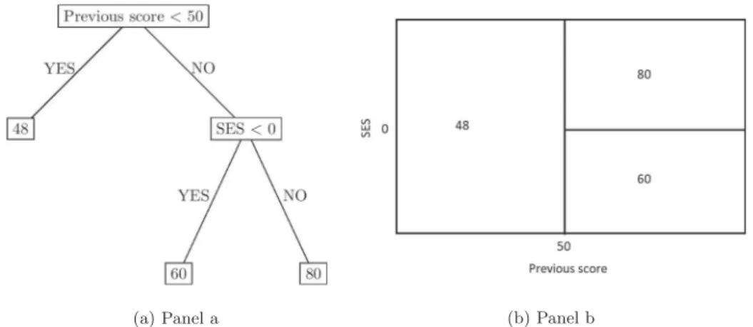
Consider the example in Figure 1 to illustrate the idea of regression trees. Imagine we want to regress student test scores (response variable) on previous scores, SES and gender (covariates). The regression tree divides the covariates space into a number of regions, where, the predicted value of the response variable within each region can be obtained as the mean of all the observations that belong to each region. The regions are identified by the model in order to minimize the residual sum of squares (RSS). In our example, the regression tree that we obtain could be displayed in Figure 1. The threshold values that are identified (previous score = 50 in the first split, SES = 0 in the second split), at each split, are able to divide the sample into subgroups, minimizing the RSS.

The tree continues to divide the covariates space into subregions until a certain criterion is reached (e.g. minimum number of observations within each region or maximum RSS within each region).

It can be the case that not all the covariates are used in the identification of regions. The covariates that are not involved are the ones that result to be not predictive for the response variable.

From the tree in Figure 2, we can conclude that, in this hypothetical example, the only variables that matter are previous test scores and SES. This implies that gender is not able to catch any variability in student test scores otherwise it would have been included in the regression tree. When estimating student test scores, we read the tree in the following way: if the previous score of the student is less than 50, then the estimated student

(a) Panel a (b) Panel b

Figure 1.Example of a regression tree (panel a), with the partition of the covariates space (panel b). The outcome variable is student test score (continuous [0,100]), and the two predictors selected by the regression tree are previous score (continuous [0,100]) and socio-economic status (continuous [−3,3]). The partition of the covariates space is done considering only the two covariates involved in the splits.

(5)

score is 48; if the previous score of the student is bigger than 50, it depends on the student SES: if the student SES is higher than 0, the expected score is 80, while if it is less than 0, the expected score is 60. Note how, in this example tree, SES only matters when the previous score was bigger than 50, indicating an interaction between previous test scores and SES. This interaction was detected by recursively partitioning the observations into nodes, and without the need to specify the interaction ex ante.

More formally, considering the regression model Y ¼fðXÞ þ, generalizing (1), the classic linear functional form is the following:

fðXÞ ¼β₀þX^j¼1

p

Xjβ_j; (3)

where X is the (n × p)-matrix of predictors, n is the number of observations andpis the number of predictors. On the other side, regression trees assume a model of the form:

fðXÞ ¼X^m^¼¹

M

cm1_ðX2RmÞ; (4)

whereR1;. . .;RM represent a partition of the covariates space and cm is the mean of all the observations that belong to region Rm. Algorithm 1 summarizes the two steps involved for building a regression tree.

Regression trees have several advantages: they do not force any functional form, they can easily model interactions among the covariates, they can easily handle categorical covariates and missing data. When modelling an EPF, regression trees are ideally suited to accommodate the hierarchical structure of education systems, characterized by interactions between (and within) different levels (e.g. see Online Figure A1 for Hungary). Despite the advantages in terms of added flexibility, regression trees have also some disadvantages: they generally suffer from high variance and are sensitive to outliers. However, there are methods that, by aggregating information from many trees into ensembles (e.g. boosting), substantially improves the predictive performance (James et al.2013).

Regression tree ensemble: boosting

Boosting is a stagewise procedure that aggregates information from many trees (=ensemble) by

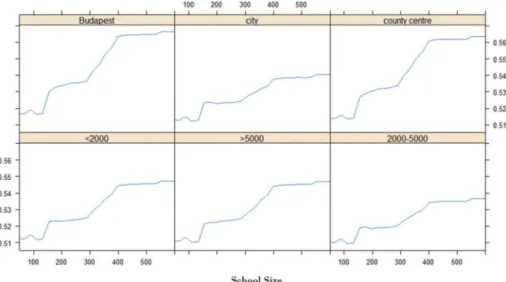
Figure 2.Joint partial plot, estimated by boosting model applied to NABC data ofLocation(categorical variable) andSchool size (continuous variable). The outcome variable is the school added value in mathematics.

Algorithm 1.Single regression trees.

1. Use recursive partitioning to divide the predictor space the set of possible values for componentsX1;X2;. . .;XpintoMdistinct and non-overlapping regions,R₁;R₂;. . .;R_M. Beingy_imtheith observation within them-region and given the mean of the observations within themth box^y_Rmthe regions are chosen in order to minimize the residual sum of squaresRSS¼P^M

m¼1

P

i2Rm

ðriÞ² where residualri¼yim^yRm.

2. For every observation that falls into regionR_m, make a prediction equal to^yRm.

(6)

growing them sequentially: each tree is grown using information from previously grown trees.

Boosting does not involve bootstrap sampling.

Instead, each tree is fit on a modified version of the original data. The idea behind this procedure is that, unlike fitting a single large tree to the data, which amounts to fitting the data hard and poten- tially overfitting (Varian 2014), the boosting approach instead learns slowly. The algorithm starts by fitting a regression tree on the original data and continuously updates it fitting regression trees on the residuals of the previous model. Given a current model, a tree is fitted on the residuals of the model, rather than on the outcome variable.

This new tree is then added into the fitted function in order to update the residuals. Note that in boosting, the construction of each tree depends strongly on the trees that have already been grown. Algorithm 2 describes this procedure.

Instead of imposing functional form assumptions on the production function, the boosting algorithm requires the specification of three parameters. First, the number of trees B.

Boosting can result in overfitting if B is too large, although this overfitting tends to occur slowly, if at all. In our application, we use cross-validation to select B.² Second, the shrink- age parameter λ, a small positive number. It is also known as the learning rate as it controls the magnitude at which each tree contributes to the model, and is typically equal to 0.01 or 0.001 (we set λ = 0.001). Third, the number of splits in each tree, d, that controls the complexity, or interaction depth, as d splits can involve at most d variables (we set d = 4).

Despite improvements in robustness by aggregating many trees, a price needs to be paid in terms of interpretability, as it is no longer possible to graphically display the final tree (as in Figure 1). Nonetheless, the output of these methods can still be informative about (i) the percentage of variability explained by the model, (ii) the variables importance (VI) ranking and (iii) partial dependence plots. The percentage of variability explained is indicated by the pseudo R². The VI ranking reveals the ranking of the covariates, based on the ‘importance’ of each covariate in explaining the response (different measures can be used to compute importance (e.g. James et al.

2013)). Focusing on the influence of each single covariate and on the interaction effects, partial dependence plots (Friedman 2001) are especially interesting as they allow us to infer the (both single and joint) relation of specific variables with the outcome. Given N observations yk, for k¼ 1;. . .;N, andppredictors, boosting generates predictions of the form:

^yk ¼Fðx1;k;. . .;xp;kÞ; (5) for some mathematical function Fð. . .Þ. The partial dependence plot, or partial plot, of the jth covariate is defined as:

ϕ_jðxÞ ¼ 1 N

X^N

k¼1

Fðx1;k;. . .;x_j1;k;x;x_jþ1;k;. . .;x_p;kÞ:

(6) ϕ_jðxÞindicates how thejth covariate is related to^y after averaging out the influence of all other variables. In other words,ϕ_jðxÞis the net effect of the jth covariate. After the identification of the important variables by means of the VI ranking, ϕ_jðxÞ allows us to investigate which is the range of values of the jth covariate that is associated to changes in the response variable and which is the form of this association. Moreover, the general- ization of this marginal effect to the multivariate case is analytically straightforward. The joint partial dependence plot, or joint plot, of the jth and ith covariates,

Algorithm 2.Boosting.

1. Set^fðxÞ ¼0 and residualsri¼yifor alliin the training set 2. Forb¼1;2;. . .;B, repeat:

(a) Fit a tree^f^bwithdsplits (dþ1 nodes) to the training data usingr_ias response variable

(b) Update^fby adding a shrunken version of the new tree:

^f ^fðxÞ þλ^f^bðxÞ

(c) Update the residuals:ri riλ^f^bðxiÞ 3. Output the boosted model:^fðxÞ ¼PB

b¼1λ^f^bðxÞ

2We use 70% of the data as a training set and setB= 3000. Online Figure C4 plots cross-validation errors against the number of trees used in the boosting model.

(7)

ϕ_i;jðx;yÞ ¼ 1 N

X^N

k¼1

Fðx1;k;. . .;xi1;k;x;xiþ1;k;. . .;

xj1;k;y;xjþ1;k. . .;xp;kÞ

(7) represents the joint effect of two covariates on ^y.

ϕ_i;jðxÞ indicates how the jth and ith covariates are related to^yafter averaging out the influence of all other variables. The advantage is that it is possible to display the joint relation of the two covariates with the outcome, showing how the two variables interact in their joint association with the response variable.

As a result, it is still possible to obtain a visual interpretation of the relationship between variables in an intuitive way. We will use these joint plots to visualize and explore interaction effects in Section IV, as an alternative approach to estimating (2).

III. Application

A trend towards more accountability in the education sector has led to the emergence of instruments to benchmark schools. The most prominent example is the VA estimate, which is considered a best practice to rank schools and has been adopted in the United Kingdom, the Netherlands and the USA.

Although VA estimates are generally preferred over raw test scores, estimating VA is a high-stakes statistical exercise, as VA estimates often determine per- sonnel decisions or school closure, and remains under debate (Koedel, Mihaly, and Rockoff 2015).

Another discussion closely related is the identification of variables that are able to explain quality (VA) differences between schools. Here, interaction effects are particularly interesting as many decisions are taken by different actors at different levels of operations (class, school, provider) (Burns and Köster 2016). As a direct consequence, not acknowledging these interactions will lead to a misrepresentation of variables and their relationship with school quality.

In this section, we illustrate the usefulness of the approach proposed above using Hungarian and

Italian datasets. In doing so, we explore the determinants of school added value, i.e. components of the EPF and interactions that determine its shape.

The boosting algorithm can be presented graphically, which facilitates interpretation. We constructed an indicator of school added value using data envelopment analysis (DEA).³ Note that this nonparametric specification overcomes the assumption that the functional form of achievement is linear and additively separable (Todd and Wolpin2003).⁴The indicator of school added value ranges between 0 and 1 and can be interpreted as the relative ability of a school to transform its inputs (prior achievement and socio-economic background) into outputs (current achievement).⁵

Data

Hungary: NABC

Our dataset for Hungary was constructed by inte- grating information on student, class and school characteristics from the National Assessment of Basic Competencies (NABC). The NABC covers all students in primary schools in Hungary (see Online Appendix A for a brief introduction to the Hungarian education system). It is a standard based assessment for mathematics and reading that follows the model of the Programme for International Student Assessment (PISA), but is conducted every year in May. Students are tested at grade 6 (age 12) and before graduation from primary school, in grade 8 (age 14). In addition to mathematics and literacy test scores, which are common in education datasets, NABC contains extensive information on school principal characteristics and the socio-economic composition of schools. This study uses data on students from the sixth grade 2008 cohort, graduating from their primary schools in grade 8 in 2010. Our main analysis is performed on school level NABC data. After the removal of statistical units with missing values, the final dataset contains

3DEA generates a frontier based on the data and allows comparison of schools with their reference school, given inputs, without any assumption on the functional form. This reference school is not the average school, but a school that is situated on the‘efficiency frontier’. The frontier for a given school consists of schools attaching the same weights to the inputs (prior achievement and socio-economic background), see Online Appendix B.

4As we are mainly interested in studying the importance of discretionary inputs (e.g. class and school size, and principal characteristics), we choose to include the socio-economic background and prior achievement in the DEA specification (see Online Appendix B).

5In order to obtain a measure of the added value of schools, input and output variables were averaged for every school. Test scores and the SES indicator are z-standardized indices, with mean 0 and standard deviation 1. The generation of this index follows the logic of the economic-social and cultural status (ESCS) index of the OECD PISA studies.

(8)

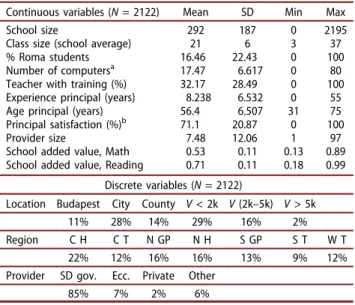
2122 schools. All variables used in subsequent analyses are presented in Table 1. A further description of the data used here can be found in Kertesi and Kezdi (2011) and OECD 2010. As can be seen in Table 1, the average added value of schools is 0.71 for reading and 0.53 for mathematics. For reading, this can be interpreted as follows: on average, a school can improve its reading achievement by 29% if it were to perform as well as its reference school.

Using information from the NABC data, we include class, school and provider size. Since our analysis is at school level,‘class size’is measured as the average class size in a school. Provider size is measured as the number of schools under super- vision of the same provider of education. In the decentralized Hungarian system, the type and size of education providers varies widely from very small local government providers with only one school to large centralized networks of church schools. Also, we include the number of computers in the

dedicated computer class, as a proxy for school resources, and the percentage of teachers receiving additional training.

Complementing the administrative data, we also include several variables from a questionnaire in NABC completed by the school principal. These additional variables can be used to describe the organizational setting of the schools. The school level questionnaire includes variables such as principal experience, age and satisfaction. Also, the perceived ratio of Roma students is indicated by the principal of each school.⁶Finally, to capture geographical discrepancies in schools’performance, we include both regional and school location categorical variables (e.g. village or city).‘School location’is a categorical variable indicating the geographical area where a school operates. Categories include Budapest, cities (not Budapest), county centres and villages (grouped by size). Summary statistics are presented inTable 1.

Italy: INVALSI

For Italy, we use data from the National Institute for the Evaluation of the Educational System of Education and Training (INVALSI). The INVALSI data closely resembles the NABC structure, albeit that students are observed in grades 5 and 8 (see Online Appendix A for a brief introduction to the Italian education system). In the application at hand, we use data for the 2013 cohort. Hence, the added value measured here reflects the added value of middle schools (‘scuola media’) as students enter school in the fifth grade and graduate from middle schools in the eighth. In contrast to the Hungarian dataset, we do not have access to comprehensive managerial and organizational variables.

Nonetheless, the dataset allows inclusion of regional variables and school characteristics. Furthermore, the INVALSI dataset contains extensive information regarding the immigration status of students. All subsequent analyses are performed on school level data. After the removal of statistical units with missing values, the final dataset contains 5751 schools.

All variables are presented inTable 2. A more comprehensive description can be found in De Simone

Table 1.Descriptive statistics for the continuous and the discrete variables in the NABC dataset, respectively.

Continuous variables (N= 2122) Mean SD Min Max

School size 292 187 0 2195

Class size (school average) 21 6 3 37

% Roma students 16.46 22.43 0 100

Number of computers^a 17.47 6.617 0 80

Teacher with training (%) 32.17 28.49 0 100

Experience principal (years) 8.238 6.532 0 55

Age principal (years) 56.4 6.507 31 75

Principal satisfaction (%)^b 71.1 20.87 0 100

Provider size 7.48 12.06 1 97

School added value, Math 0.53 0.11 0.13 0.89

School added value, Reading 0.71 0.11 0.18 0.99 Discrete variables (N= 2122)

Location Budapest City County V< 2k V(2k–5k) V> 5k

11% 28% 14% 29% 16% 2%

Region C H C T N GP N H S GP S T W T

22% 12% 16% 16% 13% 9% 12%

Provider SD gov. Ecc. Private Other

85% 7% 2% 6%

Note for the continuous variables:^aNumber of computersmeasures the total number of computers as counted in the dedicated computer class.

bPrincipal satisfactionanswers the question‘If you were to assigned to another school, what percentage of the current teaching staff would you take with you to your new place?’. Note for the discrete variables: V:

Village, N: Northern, W: Western, S: Southern, H: Hungary; T:

Transdanubia; GP: Great Plain; SD gov.: settlement or district government, Ecc.: Ecclesiastical.

6Even though it seems that the individual performance of Roma students does not differ significantly from other (non-Roma) students, once socio-economic background is accounted for (see Kertesi and Kezdi2011), the inherent discriminatory tendencies in the Hungarian society might cause some families (or even teachers) to refrain from entering schools where large Roma ratios are present. On average, 16% of students are considered to be from Roma origin.

Because of an increasingly segregated education system where so called‘Roma schools’are being ghettoized (Kertesi and Kezdi2011), the median value is much lower at 8%.

(9)

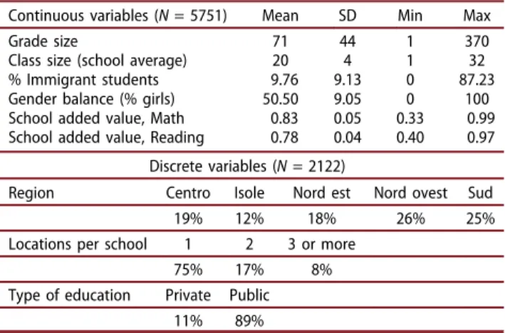
(2013, 14) or Bertoni, Brunello, and Rocco (2013, 66–67). FromTable 2, it can be seen that the average added value of schools is 0.83 for mathematics and 0.78 for reading. For mathematics, these findings suggest that school can improve their mathematics test scores by 17% if they were to perform as well as the school in their reference sets.

Summary statistics are presented inTable 2. We included school size in terms of physical locations– grade size and class size measured as the average class size in a school. In addition, we included the share of immigrants (first and second generation combined), and the gender balance of the school, calculated as the share of girls. To capture well- documented geographical discrepancies in educational outcomes in Italy (e.g. Agasisti, Ieva, and Paganoni2017), we also consider regional dummies.

Finally, we included a dummy indicating whether schools are privately or publicly organized.

Results

In this section, we graphically display the results of the application of boosting to both the Hungarian and Italian data, when school added value in mathematics is the outcome variable and the school level

variables shown in the previous section are the predictors.⁷In order to allow a comparison of models, we included the output of ordinary least squares (OLS) regressions in Tables 3 and 4. Using the boosting approach, the importance of variables in explaining the added value of schools can be ranked (see Section‘Regression tree ensemble: boosting’).⁸ Finally, we present joint plots to visualize interactions between explanatory variables and the added value of schools. Joint plots display a net effect, accounting for all other control variables in the model. In order to allow an intuitive interpretation, boosting requires choosing two variables and dis- plays their joint plot.⁹It is important to note that this choice does not affect the model outcome. In fact, the structure of the model (seeFigure 1) assures that interactions within and between levels are included by construction. As a result, no assumptions will be needed on the existence and functional form of interaction effects. In this vein, we can interpret the results in the joint plots as a data-driven estimation of possibly nonlinear interactions between components of the EPF. The outcome variable for all joint plots is the added value of schools in mathematics, where the mean is set to 0 in order to ease the interpretation.

Hungarian schools

In Figures 2 and 3, we present three examples of variable combinations to illustrate how boosting can be used to explore heterogeneous effects in an intuitive way.¹⁰Corresponding OLS coefficients are presented in Table 3 (A, B, C and D). Regression A presents the baseline model, without interactions. It includes size variables (class, school and provider), the share of Roma students, the number of computers, principal characteristics (age, experience, satisfaction), in addition to dummies for school location, the type of education provider and region. All subsequent models (B, C and D) extend the baseline model by adding an interaction effect. This way, the regression results can be easily compared to the

Table 2.Descriptive statistics for the continuous and the discrete variables in the INVALSI dataset, respectively.

Continuous variables (N= 5751) Mean SD Min Max

Grade size 71 44 1 370

Class size (school average) 20 4 1 32

% Immigrant students 9.76 9.13 0 87.23

Gender balance (% girls) 50.50 9.05 0 100

School added value, Math 0.83 0.05 0.33 0.99

School added value, Reading 0.78 0.04 0.40 0.97 Discrete variables (N= 2122)

Region Centro Isole Nord est Nord ovest Sud

19% 12% 18% 26% 25%

Locations per school 1 2 3 or more

75% 17% 8%

Type of education Private Public

11% 89%

Note for the discrete variables: Locations per schooldenotes the number of physical locations (or‘plessos’) supervised by one administrative unit.

7Results for reading are analogous and hence left out for the sake of brevity.

8The relative importance of variables in the EPF, as modelled by boosting, is displayed in Online Figure C1. Online Figure C2 presents partial plots for the share of Roma students, school size, school location and class size, identified as important determinants of school added value in Hungary. Online Figure C3 presents partial plots for the share of immigrants, grade size, school region and class size, identified as important determinants of school added value in Italy. Partial plots display the partial influence of a variable on the outcome, averaging out the influence of all other variables included in the model. This graphical approach can be compared to plotting the OLS coefficients obtained inTables 3and4, without assuming this coefficient is constant (or varies at given rate) across values of a specified variable.

9Selecting three variables would be possible if a 3D plot is used.

10Additional joint plots and alternative variable combinations, together with the R code are available upon request.

(10)

boosting approach. In terms of model fit, the boosting approach outperforms the linear regression model (pseudo R² of 24.9 compared to an R² of 21.9 for OLS). This model improvement, as measured byR², might be due to the actual relationships not being linear (Varian2014).

In Figure 2, we interact a categorical and a continuous variable, school location and school size, with the aim of showing how our variable

of interest (school VA) is jointly affected by the two variables. Although the shape of the relationship in all school locations looks similar, its strength can be seen on the vertical axis, indicating a strong discrepancy across locations. For example, the variation in added value related to school size differences appears to be much smaller in cities compared to county centres and Budapest, as showed by the steeper slope of the line measuring the outcome of interest. This might indicate that school size reform could have a differential impact across school locations, confirm- ing the need to account for heterogeneous effects.

OLS results indicate a similar pattern but compli- cate the interpretation, as is often the case in empirical studies (Hainmueller, Mummolo, and Xu 2017). When schools in cities are set as the reference category, we can see from B that the school size slope is significantly steeper for schools in Budapest and county centres. The coefficient on school size is now close to 0 and no longer significant. This does not imply that the unconditional effect is no longer significant after including interactions in the specification, it simply captures the school size effect in cities (i.e. the reference category, or Z = 0), i.e. averaging effects that instead are heterogeneous across the school size

Table 3.Results of the OLS regression model applied to NABC data.

Variables A B C D

School size 0.001*** 0.000 0.001*** 0.001***

Average class size 0.011** 0.0100** 0.011** 0.011**

Roma students −0.014*** −0.014*** −0.012*** −0.014***

Number of computers 0.003 0.003 0.002 0.003

P age −0.006* −0.006* −0.006* −0.006

P experience 0.012*** 0.012*** 0.001*** 0.013

P satisfaction 0.001 0.001 0.001 0.001

Provider size 0.004 0.004 0.004 0.004

Interactions (Reference = Cities)

Budapest × School size 0.001***

County centre × School size 0.001***

Village (<2k) × School size 0.000

Village (2k–5k) × School size −0.000

Village (>5k) × School size 0.000

Roma students × School size −0.000***

P experience × Age 0.000

Constant 0.844*** 0.778*** 0.423 0.837**

Controls

School location X X X X

Education provider X X X X

Region X X X X

Observations 2122 2122 2122 2122

R² 0.213 0.221 0.221 0.219

Note: P: principal,Provider sizeindicates the number of schools affiliated to a district, as inTable 1. The outcome variable is the added value of schools in terms of mathematics.

*, **, *** indicate significance at the 10%, 5% and 1% level, respectively.

For conciseness, standard errors are not displayed here.

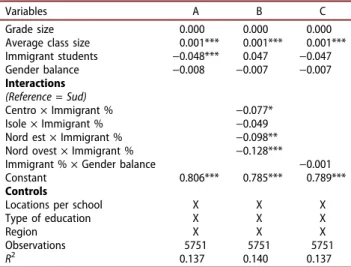
Table 4.Results of the OLS regression model applied to INVALSI data .

Variables A B C

Grade size 0.000 0.000 0.000

Average class size 0.001*** 0.001*** 0.001***

Immigrant students −0.048*** 0.047 −0.047

Gender balance −0.008 −0.007 −0.007

Interactions (Reference = Sud)

Centro × Immigrant % −0.077*

Isole × Immigrant % −0.049

Nord est × Immigrant % −0.098**

Nord ovest × Immigrant % −0.128***

Immigrant % × Gender balance −0.001

Constant 0.806*** 0.785*** 0.789***

Controls

Locations per school X X X

Type of education X X X

Region X X X

Observations 5751 5751 5751

R² 0.137 0.140 0.137

Note: The outcome variable is the added value of schools for mathematics.

*, **, *** indicate significance at the 10%, 5% and 1% level, respectively.

For conciseness, standard errors are not displayed here.

(11)

distribution. In order to obtain an estimate of the unconditional school size effect, we need to add up coefficients for all categories, weighted by their relative frequency. Although the coefficients for each location are not included in Table 2, interpreting them in B would be nonsensical as there are no schools without students. Also, the insignificance of the coefficient for school size in this specification, and the insignificance of some interaction effects does not imply that the unconditional school size effect is insignificant, but only

that ‘average’ effects do not reveal the complex

heterogeneous effect of the two joint variables over the outcome of interest.

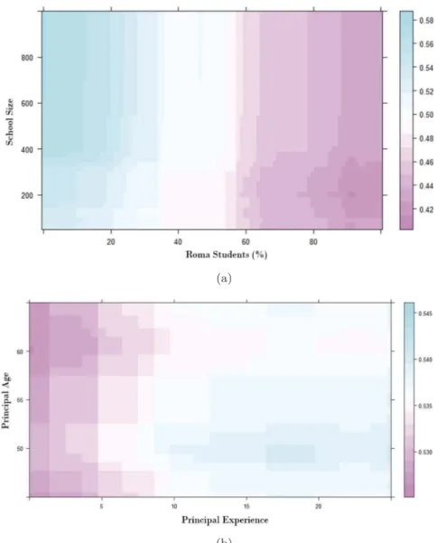
As another example, the joint plots inFigure 3 interact two continuous variables: % Roma students and school size (top), and principal age and experience (bottom). The added value of schools is now indicated using a colour scale, ranging from blue (high) to purple (low). The colours correspond to schools characterized by the interaction of two variables indicated on the axes. In this perspective, the areas of the graph where the colour is more intense (blue) are those where schools report higher VA, and reading their partitioning can reveal their characteristics about joint levels of percentage of Roma students and size. Clearly, the highest added value can be found

(a)

(b)

Figure 3.Joint partial plot, estimated by boosting model applied to NABC data of School size and Roma students (%) (a) and Principal AgeandPrincipal Experience(b). In both the plots, the outcome variable is the school added value in mathematics. The joint plot can be interpreted as follows: the lighter the colour, the more pronounced the added value of the school in mathematics at this specific point. Each point in every graph corresponds to an intersection of two values of the variables denoted on the horizontal and vertical axes.

(12)

in relatively large schools with a low share of Roma students. The joint plots allow us to explore, possibly nonlinear, interaction effects. For example, in schools where the share of Roma students is rather low, a clear positive relationship between school size and added value can be seen in Figure 3, while schools with a majority of Roma students seem to be adding more value in relatively small and large schools. Middle-sized schools with many Roma students appear to perform the worst in terms of added value. Perhaps highly segregated schools benefit from either a tailored approach facilitated by a smaller school size, or from scale economies experienced by lar- ger schools. From Table 3C, we find that the interaction effect Roma students × School size is significantly negative, indicating that the positive school size effect (seeTable 3A) is decreasing with the share of Roma students. Although we do not claim to present a causal relationship, it is clear from this comparison that joint plots reveal patterns that cannot be obtained using multiplicative interactions, which instead are able only to represent average effects, i.e. in the middle of the distribution of the variable of interest.

The bottom panel of Figure 3 interacts the age and experience of school principals. In contrast to the top panel, and Figure 2, no clear interaction effect can be observed between age and experience. Nonetheless, interacting two continuous variables in joint plots allows us to identify an

‘optimum’: schools led by a relatively young (50 years) and experienced (around 17 years) principal. In this vein, the figure can be used to obtain information about the complexity of the interactions between two continuous variables, whose relationship is not linear along the whole distribution of each of them. The difference between these schools and schools led by relatively old (60 years) and inexperienced principals amounts to 15% points in school added value. In addition, and in contrast to coefficients from Table 3D, the graphical approach reveals a cutoff around 10 years, where the added value of schools

‘jumps’to higher values. Consistent with this find- ing, it has been argued before that school principals‘take time to realize their full effect at schools’

(Coelli and Green 2012, 92). Again, the graphical approach proposed here reveals interesting

patterns, which cannot be obtained from Table 3, where the coefficient for the variable Principal experience × Principal age actually measures the non-statistically effect on school value-added, that is easily observable in the white cells in the middle of the graph reported in Figure 3(b).

Italian schools

In order to illustrate the wider applicability of the proposed approach to visualize interaction effects, we repeat the methodological approach of our analysis using Italian data described in ‘Results’

section. Regression A presents the baseline model, without interactions. It includes size variables (grade and class), the share of immigrant student, the gender balance, and dummies for the number of locations per school (1, 2 and 3 or more), the type of education (public or private), and the geographical region. Subsequent models B and C extend the baseline model by adding an interaction effect. This way, the regression results can be easily compared to the boosting approach.

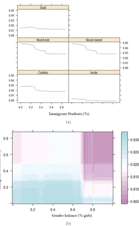
In terms of model fit, the boosting approach again outperforms the linear regression model (pseudo R²of 15.9 compared to an R² of 14.0 for OLS). As noted before, this model improvement, might be due to the actual association not being linear (Varian 2014). Figure presents two examples of variables combinations and their joint relationship with the added value of Italian schools. As in Figure 2 for Hungary, we interact a categorical and a continuous variable in Figure 4(a): region and immigrant students (%). Both the shape and the position of the relationship between school added value and the share of students from an immigrant background appears to depend on the region where a school is located, as it appears evident from the different shapes of the plots in the different quadrants. On the one hand, the discrepancies in Figure 4(a) capture regional differences in added value between schools. On the other hand, this figure suggests differential effects of immigrant students on the added value of schools, depending on the region, corroborating the need for a more nuanced view of marginal effects. Looking at Table 4, the OLS results (Table 4B) suggest a similar pattern, i.e. all slopes are more negative compared to the reference

(13)

region (Sud), although this difference is not significant for Isole. Again, complications arise in terms of interpreting the constitutive terms, because of their value in interpreting ‘average effects’ and not the whole distribution of the effects of the variable of interest on outcome, which is overcome by the intuitive graphical approach.

Figure 4(b) presents the joint plot of the interaction between two continuous variables in influ- encing the outcome of interest (school VA): the gender balance (% girls) and the share of students from an immigrant background. As before, the colour scale represents the added value of schools.

In contrast to Figure 3, no clear interaction effect can be observed here. However, as inFigure 4(a)

(a)

(b)

Figure 4.Joint partial plots, estimated by boosting model applied to INVALSI data, ofGeographical location(categorical variable) andImmigrant students (%)(continuous variable) (a) andPrincipal Age andPrincipal Experience(both continuous variables) (b). In both the plots, the outcome variable is the school added value in mathematics. The joint plot in panel (b) can be interpreted as follows: the lighter the colour, the more pronounced the added value of the school in mathematics at this particular point.

(14)

the graphical approach reveals interesting patterns, which cannot be obtained from Table 4.

For example, schools with the highest added value in mathematics are those schools whose students are mainly boys and do not come from an immigrant background. On the contrary, schools consisting of mainly girls with an immigrant background appear to perform the worst.

Finally, schools with mostly immigrant boys (top left) are adding value in mathematics to their students, roughly equivalent to schools that con- sist of mostly girls without an immigrant background (bottom right). Although we do not claim to provide any causal evidence on this matter, this example once again illustrates the exploratory benefits of visualizing how variables interact to determine an outcome. In particular, the graph allows to visualize those cases where the joint effect of two variables is associated with higher school VA (darker colour), avoiding the risk of capturing a ‘zero effect’ in the middle of the distribution of the two interacted variables where the colour of the relationship is lighter.

IV. Conclusion

This article demonstrates how regression trees and ensembles can be used to model and visualize interaction effects. Multiplicative interactions are commonly used to identify heterogeneous treatment effects and to tailor policy recommendations. The method proposed in this article provides applied economists with an innovative tool to explore interaction effects in a way that overcomes common specification and interpretation errors. Our empirical application illustrates the usefulness of joint plots generated by the boosting algorithm to model interaction effects in education. For example, we find that school size has different effects on the added value of schools, depending on the socio-economic composition and location of schools. This means that the effect of each predictor might depend also on the values of the other predictors, suggesting that, when making considerations about each single aspect of schools, its effect needs to be related to the setting in which it acts. Visualizing results in joint plots allows an intuitive interpretation of interaction effects.

Despite the complexity of the model, results can be easily read, while at the same time, flexible

interactions provide a more realistic insight into the (education) production function. As illustrated using two datasets, a potential data-driven approach can be derived. Practitioners could explore relationships between variables using the boosting algorithm and visualize them, before formally testing interactions in a regression framework. In many applications, boosting and regression could prove complementary to uncover and test complex relationships.

Acknowledgements

We are grateful to Kristof De Witte, Geraint Johnes, Daniel Santin, and other seminar participants in Milan, Lisbon, Leuven, Sankt Gallen, and Budapest for many useful com- ments and remarks and to Anna Maria Paganoni for statistical discussions during the analysis.

Disclosure statement

The authors declare that they have no relevant or material finan- cial interests that relate to the research described in this article.

Funding

The project leading to this article has received funding from the European Union’s Horizon 2020 Research and Innovation Programme under grant agreement no. 691676 (EdEN).

ORCID

Fritz Schiltz http://orcid.org/0000-0001-9920-5353

References

Agasisti, T., F. Ieva, and A. M. Paganoni. 2017.

“Heterogeneity, School-Effects and the North/South Achievement Gap in Italian Secondary Education:

Evidence from a Three-Level Mixed Model.” Statistical Methods & Applications26 (1): 157–180.

Ai, C., and E. C. Norton.2003.“Interaction Terms in Logit and Probit Models.”Economics Letters80: 123–129.

Angrist, J., P. Azoulay, G. Ellison, R. Hill, and S. F. Lu.2017.

“Economic Research Evolves: Fields and Styles.”American Economic Review107 (5): 293–297.

Berry, W. D., M. Golder, and D. Milton.2012. “Improving Tests of Theories Positing Interaction.” The Journal of Politics74 (3): 653–671.

Bertoni, M., G. Brunello, and L. Rocco.2013.“When the Cat Is Near, the Mice Won’t Play: The Effect of External

(15)

Examiners in Italian Schools.”Journal of Public Economics 104: 65–77.

Blumenstock, J. E. 2016. “Fighting Poverty with Data.” Science353 (6301): 753–754.

Brambor, T., W. R. Clark, and M. Golder. 2006.

“Understanding Interaction Models: Improving Empirical Analyses.”Political Analysis14 (1): 63–82.

Burns, T., and F. Köster. 2016. “Governing Education in a Complex World. OECD Publishing. Chalfin, A., Danielli, O., Hillis, A., Jelveh, Z., Luca, M., Ludwig, J., And Mullainathan, S. (2016). Productivity and Selection of Human Capital with Machine Learning.” American Economic Review106 (5): 124–127.

Coelli, M., and D. A. Green. 2012. “Leadership Effects:

School Principals and Student Outcomes.” Economics of Education Review31 (1): 92–109.

De Simone, G. 2013. “Render Unto Primary the Things Which are Primary’s: Inherited and Fresh Learning Divides in Italian Lower Secondary Education.” Economics of Education Review35: 12–23.

Friedman, J. H.2001. “Greedy Function Approximation: A Gradient Boosting Machine.” Annals of Statistics 29 (5):

1189–1232.

Hainmueller, J., J. Mummolo, and Y. Xu (2017). How Much Should We Trust Estimates from Multiplicative Interaction Models? Simple Tools to Improve Empirical Practice.Working Paper.

James, G., D. Witten, R. Hastie, and R. Tibshirani.2013.An Introduction to Statistical Learning. Springer. New York: 6 edition.

Karaca-Mandic, P., E. C. Norton, and B. Dowd. 2012.

“Interaction Terms in Nonlinear Models.”Health Services Research47: 255–274.

Kertesi, G., and G. Kezdi.2011. “The Roma/Non-Roma Test Score Gap in Hungary.”American Economic Review101 (3):

519–525.

Kleinberg, J., H. Lakkaraju, J. Leskovec, J. Ludwig, and S.

Mullainathan. 2017. “Human Decisions and Machine Predictions.” Quarterly Journal of Economics 133 (1):

237–293.

Koedel, C., K. Mihaly, and J. E. Rockoff.2015.“Value-Added Modeling: A Review.”Economics of Education Review47:

180–195.

Nowak, A., and P. Smith. 2017. “Textual Analysis in Real Estate.”Journal of Applied Econometrics32 (4): 896–918.

OECD (2010). OECD Review on Evaluation and Assessment Frameworks for Improving School Outcomes Hungary Country Background Report. Technical report, OECD, Paris.

Su, X., K. Meneses, P. McNees, and O. Johnson. 2011.

“Interaction Trees: Exploring the Differential Effects of an Intervention Programme for Breast Cancer Survivors.” Journal of the Royal Statistical Society. Series C (Applied Statistics)60 (3): 457–474.

Todd, P. E., and K. I. Wolpin. 2003. “On the Specification and Estimation of the Production Function for Cognitive Achievement.”Economic Journal113 (485): F3–33.

Vanthienen, J., and K. De Witte. 2017. Data Analytics Applications in Education. Boca Raton, FL: Taylor & Francis.

Varian, H. R.2014.“Big Data: New Tricks for Econometrics.” The Journal of Economic Perspectives28 (2): 3–28.