Handout Probability

(1)

EFOP-3.4.3-16-2016-00014

Probability

Handout

Prepared by

János Marcell BENKE, PhD Methodological expert: Edit Gyáfrás

This teaching material has been made at the University of Szeged and supported by the European Union. Project identity number: EFOP-3.4.3-16-2016-00014

2020

Szegedi Tudom´anyegyetem

C´ım: 6720 Szeged, Dugonics t´er 13.

(2)

Preface

Probability incorporates two courses: the related lecture and the seminar. The aim of these courses is to teach the meaning of the basic notions of probability theory as probability, random variables, probability distribution, expected value, standard deviation, variance, covariance, density function, normal distribution.

This handout presents the definitions and theorems applied during the semester and provides examples for better understanding and for practicing and also includes sample tests. The starred exercises are a slightly more difficult then the others. Problems like these will not appear in the tests.

Lecturer: J´anos Marcell BENKE

(3)

Course information

Course title: PROBABILITY

Course code:

60A106 Lecture 60A107 Seminar

Credit: 3 + 2

Type: lecture and seminar

Contact hours / week: 2 + 1

Evaluation:

Lecture: exam mark (five-grade) Seminar: practical course mark (five-grade)

Semester: 3^rd

Prerequisites: Calculus

(5)

Learning outcomes

(a) regarding knowledge, the student

- can use basic combinatorical counting methods as permutation, variation and combination to count the number of possible outcomes of an experiment

- is able to simplify complex events using operations on events - knows the definition of probability and the heuristic of it as well - can calculate probabilities on classical probability space

- can calculate probabilities of events connected to discrete random variable using its probability distribution

- can calculate expected value, standard deviation, variance of discrete random variable using its probability distribution

- understands the heuristical meaning of expectation and standard deviation - understand the meaning of covariance and correlation

- is able to identify binomial, hypergeometric and geometric distribution - understands the meaning of conditional probability and is able to calculate it - can calculate probabilities of events connected to continuous random variable

using its probability density function

- can calculate expected value, standard deviation, variance of continuous random variable using its probability density function

- can calculate probabilities of events connected to normally distributed random variable

- can calculate approximated probabilities using normal distribution (b) regarding skills, the student

- can uncover facts and basic connections

- can draw conclusions and make critical observations along with preparatory sug- gestions using the theories and methods learned

(c) regarding attitude, the student

- behaves in a proactive, problem oriented way to facilitate quality work

- is open to new information, new professional knowledge and new methodologies (d) regarding autonomy, the student

- conducts the tasks defined in his/her job description independently under general professional supervision

- takes responsibility for his/her analyses, conclusions and decisions

(6)

Requirements

During the semester there are 5 small tests and each small test is worth 5 points. There is no way to retake any of the small tests. Based on the collected points the following grade is given for the seminar:

1: 0-5 points, 2: 6-8 points, 3: 9-11 points, 4: 12-14 points, 5: 15-25 points.

The examination is a big test, which can be written in the exam period. It is worth 50 points. It is profitable to collect more points from the small test, because the points over 15 will be added to the big test points. Based on the collected points the following grade is given for the lecture:

1: 00-19 points, 2: 20-26 points, 3: 27-33 points, 4: 34-39 points, 5: 40-50 points.

Example: in the case of 20/25 small test points and 37/50 big test points, the seminar mark is 5, and the overall point is 5+37=42, so the lecture mark is 5 as well.

(7)

Course topics

Combinatorial counting methods, basic properties of probability, classical probability space, conditional probability. Discrete random variables, expectation, variance. Continuous random variables. Moments, skewness, curtosis, median and quantiles. Law of large numbers and central limit theorem.

(8)

1 Counting methods

When calculating probabilities we often have to rely on combinatorial methods to find the total number of possible outcomes of a random experiment. In this chapter we are going to refresh these methods, and introduce (standard) notations for them.

Definition 1.1 (Factorial). The factorial of a non-negative integer n, denoted by n!, is the product of all positive integers less than or equal to n, that is

0! := 1, n! :=

n

Y

i=1

i= 1·2·. . .·n, n>1.

Permutations of different objects

Proposition 1.2 (Permutations without repetition). Suppose we have n different objects, then we can arrange them in order in n! different ways.

Proof. We have n choices for the first element of the sequence, then we have only n−1 choices for the second element, because we are allowed to use the same object only once.

For the third element we haven−2 choices, and so on. Multiplying these numbers together

gives the desired result.

Example 1.3. How many ways can we rearrange the letters of the word MATH?

Solution. Since the word MATH consists of 4 distinct letters, the number of permutations of these letters is 4! = 24. It is such a small number, that we can list all those rearrangements:

MATH MAHT MTAH MTHA MHAT MHTA

ATHM ATMH AHTM AHMT AMTH AMHT

THAM THMA TAMH TAHM TMAH THHA

HMAT HMTA HTAM HTMA HATM HAMT

Example 1.4. A deck of French playing cards consists of 52 cards, one card for each of the possible rank and suit combinations, where there are 13 ranks namely 2, 3, 4, 5, 6, 7, 8, 9, 10, Jack, Queen, King, Ace and four suits Clubs(♣), Diamonds(♦), Hearts(♥), Spades(♠). If we shuffle this deck of cards what is the number of possible outcomes?

Solution. Since each card in the deck is unique, we have 52 different objects, therefore the number of possible permutations is 52!≈8.065·10⁶⁷. That is a huge number with 68 digits. It would be futile to try to list all the possible outcomes.

Permutations of not necessarily different objects

Our method fails to give the correct answer if the objects we aim to rearrange are not unique. In order to find all the rearrangements of the letters of the word FOOD we need to refine our way of calculating permutations.

Proposition 1.5 (Permutations with repetition). Suppose we have ` >0 types of objects.

We take k₁ of object 1, k₂ of object 2, and so on k_` of object `, a total of n=k₁+· · ·+k_` objects. The number of permutations these objects have is

n!

k₁!k₂!·. . .·k_`!.

(9)

Note that if we only have 1 of each object then we get back the statement of Proposition 1.2, since 1! = 1. We will not prove this proposition, however we will illustrate the idea of the proof in the following example.

Example 1.6. How many ways can we rearrange the letters of the word FOOD?

Solution. First we assume that we have a way to distinguish the 2 letters O, for example we can use a different colour for them. Then we have 4 different letters, and we already know the number of rearrangements is 4! = 24. We list them to illustrate the point

DFOO DFOO DOFO DOFO DOOF DOOF

FDOO FDOO FODO FODO FOOD FOOD

ODFO ODFO ODFO ODFO ODOF ODOF OODF OODF OOFD OOFD OFOD OFOD

The problem is, that we have counted some words more than once. In fact we have counted each word twice! The reason for this is that we have two choices when we select which letter O has red colour. Therefore the correct answer, the number of possible rearrangements of the letters FOOD is 4!/2 = 12. Since 2! = 1·2 = 2 that is the same answer we get using

Proposition 1.5.

Example 1.7. How many ways can we rearrange the letters of the word MATHEMATICS?

Solution. The word mathematics consists of 11 letters, but the letters A, M, and T appear twice. Using Proposition 1.5 we get that the number of possible rearrangements are

11!

2!·2!·2! = 4989600.

Variations of objects

Previously we were limited by the number of available objects of each type. If we allow ourselves the option to use each object as many times as we wish, then the number of possible sequences we can make are infinite, however if we restrict ourselves to sequences of a given length the answer becomes finite.

Proposition 1.8 (Variations with repetition). Suppose we have n >0 types of objects. If we are allowed to use each object multiple times, then the number of sequences of length

` >0 we can create using these objects is n^`.

Proof. We have n choices for the first element of the sequence, then we have the same n choices for the second element, because we are allowed to use the same object more than once. This gives us n choices for each of the ` elements of the sequence, multiplying them

together gives the desired result.

Example 1.9. How many 3 digit numbers can we make using the digits 1,4,7 if we can

(10)

111 114 117 141 144 147 171 174 177 411 414 417 441 444 447 471 474 477 711 714 717 741 744 747 771 774 777

Example 1.10. We roll a dice twice, list all the possible outcomes!

Solution. A dice has 6 sides marked with numbers 1, 2, 3, 4, 5, 6, that is our n = 6 different objects. We roll the dice twice, that means we are looking for sequences of length

`= 2. Therefore the number of these outcomes is n^` = 6² = 36. Here we list them (1,1) (1, 2) (1, 3) (1, 4) (1, 5) (1, 6)

(2,1) (2, 2) (2, 3) (2, 4) (2, 5) (2, 6) (3,1) (3, 2) (3, 3) (3, 4) (3, 5) (3, 6) (4,1) (4, 2) (4, 3) (4, 4) (4, 5) (4, 6) (5,1) (5, 2) (5, 3) (5, 4) (5, 5) (5, 6) (6,1) (6, 2) (6, 3) (6, 4) (6, 5) (6, 6)

Note that we included both (1, 2) and (2, 1) in our list, that is because we care about the order in which these numbers appear. There are cases when we don’t need information about the order. One such case is discussed in the next subsection.

Combination without repetition

So far we cared about the order of things, but this time we study questions where the order of things is irrelevant. For example in a game calledpoker, each player draws 5 cards from a shuffled deck of French playing cards and after some betting (which we ignore here, thus vastly simplifying the game) the player with the most powerful combination of cards wins. The combination called royal flush is a hand of 5 cards with the ranks 10, Jack, Queen, King and Ace with the same suit, it is the most powerful one as it beats all other combinations and ties with another royal flush. In order to study the number of different poker hands we have to introduce the binomial coefficient.

Definition 1.11. Let n∈Na positive integer, and 0 ≤k≤n another integer, then then choose k binomial coefficient is denoted by ⁿ_k

and can be calculated as n

k

= n!

k!(n−k)!.

Proposition 1.12 (Combination without repetition). A set with n unique elements has

n k

different subsets of size k, that is, if we have n different objects, then we can choose k of them in ⁿ_k

ways.

Proof. We are going to use permutations to demonstrate this. Suppose we select the objects by taking a permutation of the n elements, and taking the first k objects of that ordering. Then we have n! permutations, however not all of them produce a different selection, because the order of the firstk and lastn−k elements don’t matter. So we have counted each selectionk!(n−k)! times, dividing with this number gives the desired result.

(11)

Example 1.13. Suppose we want to make pizza. Our basic pizza will have tomato sauce and cheese but we want additional toppings. How many different pizzas can we make using exactly two of the four available toppings: ham, pineapple, corn, mushroom?

Solution. The previous proposition gives us the correct result 4

2

= 4!

2!(4−2)! = 24 4 = 6.

In order to illustrate the idea of the proof, we are going to list the permutations and the pizzas we can create using them. Let H, P, C, and M denote ham, pineapple, corn and mushroom respectively. Then we can list all possible permutations and the pizzas we would make using those permutations as a basis

HPCM HPMC PHCM PHMC −→ {ham, pineapple}

HCPM HCMP CHPM CHMP −→ {ham, corn}

HMCP HMPC MHCP MHPC −→ {ham, mushroom}

PCHM PCMH CPHM CPMH −→ {pineapple, corn}

PMHC PMCH MPHC MPCH −→ {pineapple, mushroom}

CMHP CMPH MCHP MCPH −→ {corn, mushroom}

Example 1.14. How many poker hands are possible, that is how many ways can we draw 5 cards out of a deck of french playing cards?

Solution. Using the n choose k formula, all we have to do is substitute n = 52, the number of cards in the deck, and k = 5, the number of cards we are drawing. Then the answer we are looking for is

52 5

= 52!

5!47! = 48·49·50·51·52

5! = 2598960.

Example 1.15. The most famous Hungarian lottery system is called ötöslottó, and it is a game of luck, where you can buy a ticket for some amount of money (at the time of writing this, it is 225 Hungarian forints) where you have to mark 5 numbers out of 90.

At each weekend the company responsible for the lottery randomly generates 5 numbers out of 90, and gives out prizes for those who guessed at least 2 of them correctly on their ticket. While the prize for guessing only 2 numbers correctly is only a small amount of money, guessing all 5, thus hitting the jackpot makes the winner wealthy. How many ways can we fill out a lottery ticket, that is how many different tickets should we fill out, if we want to guarantee a jackpot?

Solution. Using thenchoosekformula, all we have to do is substituten= 90, the number of numbers on the ticket, and k = 5, the number of guesses we have to make. Then the answer we are looking for is

(12)

This is not a winning strategy as the total price of those tickets would be much more than the jackpot of a lottery game. Even if the jackpot would be greater than the price, we would face at least two problems. In case of multiple winners the prize is split evenly and even if no one fills out all the possible tickets someone might get lucky and ruin our investment. Also filling out the tickets would be no small task, filling out 1 ticket per second (an unreasonable speed) it would take 43949268 seconds, roughly 1 years and 5 months of non-stop work.

Further readings:

• https://en.wikipedia.org/wiki/Pascal%27s_triangle

• https://en.wikipedia.org/wiki/Poker

• https://en.wikipedia.org/wiki/Lottery

(13)

1.1 Exercises

Problem 1.1. How many ways can we rearrange the letters of the word PROBLEM?

Problem 1.2. How many four digit numbers can we create using the digits 1,3,5,6, if we can only use each digit once? How many even four digit numbers can we create using the same digits? What is the answer to these questions if we can use the same digits more than once?

Problem 1.3. A group of friends Emma, Jennifer, Peter, Sam and Adam go to the cinema to watch the movie The Lion King. They have tickets for seat numbers 3 to 7 in the 8th row. How many ways can they be seated? How many ways can they be seated if Emma sits next to Sam?

Problem 1.4. How many ways can we rearrange the letters of the word EXERCISES?

Problem 1.5. How many four digit numbers can we create using the digits 1,2,2,6? How many odd four digit numbers can we create using the same digits?

Problem 1.6. We have 5 red, 3 green and 3 yellow balls. How many ways can we arrange them?

Problem 1.7. How many ways are there to order three scoops of ice cream in a cone if the shop sells 12 different flavours of ice cream? (Suppose that the order of scoops matter.) Problem 1.8. How many possible outcomes does the experiment of rolling a dice 10 consecutive times have?

Problem 1.9. The local florist sells 5 different kinds of flowers. We’d like to surprise someone with a bouquet made from two different kinds of flowers. How many ways can we do that?

Problem 1.10. How many ways can we select a student council with 3 equal members out of a class of 31 students? How many can we select a student council consisting of a president, a secretary, and a spokesman with different responsibilities out of a class of 31?

(Note that no student can hold more than one title of the student council.)

Problem 1.11. The deck of 52 French playing cards is the most common deck of playing cards used today. It includes thirteen ranks of each of the four French suits; clubs(♣), diamonds(♦), hearts(♥), spades(♠). We shuffle the deck and draw 5 cards from it. How many possible 5 card hands can we get? (We don’t care about the order of the cards drawn just the cards themselves.)

The final answers to these problems can be found in section 10.

(14)

2 Probability

Probability is the branch of mathematics that models randomness. Therefore we need a concept of randomness before we can talk about probabilities of events.

Sample space, events

Definition 2.1 (Random experiment). By a random experiment we mean an experiment that has the following properties

• The possible outcomes are known.

• The outcome of the experiment is not predictable in advance.

• The experiment can be repeated under the same circumstances an arbitrary amount of times.

The first two requirements seem reasonable as we want to speculate about the future, for that we need to know what can happen, but we have to be uncertain as to what will happen. In order to make sense of the third requirement we are going to introduce events and their relative frequencies.

Definition 2.2 (Sample space). The sample space is the set of all possible outcomes of a given random experiment. We denote it by Ω.

We introduce events in an intuitive way. An event is a statement about the outcome of a random experiment whose truth can be decided after carrying out the experiment. Since this representation is not unique (we are going to see this in the first example) we need a unique way to describe an event, and that is going to be the set of outcomes which satisfy the statement.

Definition 2.3 (Event). Let Ω be the sample space of a random experiment, then the subsets of Ω are called events.

For absolute mathematical precision we would have to restrict our definition of events to certain subsets of the sample space, but that is only relevant in cases where the sample space is infinite. Since we almost always use a finite sample space during this subject we are going to omit this considerations.

Definition 2.4. Let Ω be any set. Then we call the set that contains all subsets of Ω the power set of Ω, and we denote it by 2^Ω.

Every event is an element of the power set of the sample space of the related random experiment. We say that the event A ⊂ Ω occurs or happens if after carrying out the experiment the outcome is in A.

Definition 2.5. There are two events corresponding to the always false and the always true statements that we give special names. We call the event represented by the set Ω the certain event, while we call the event corresponding to the empty set,∅the impossible event.

Example 2.6. Describe the random experiment related to tossing a coin once, and ob- serving whether it lands on heads or tails! Find the set representation for the following statements!

(15)

• The coin lands on heads.

• The coin lands on tails.

• The coin does not land on tails.

Solution: The experiment has two possible outcomes, heads or tails, so Ω ={heads, tails}.

We can create a table listing all the possible outcomes in the columns and the statements in the rows, and write true or false if the corresponding statements is true or false for the give outcome.

heads tails The coin lands on heads. true false The coin lands on tails. false true The coin does not land on tails. true false

From this table we can simply list for each statement the set of outcomes which has true assigned to them and we get the following.

The coin lands on heads. −→ {heads}

The coin lands on tails. −→ {tails}

The coin does not land on tails. −→ {heads}

As we can see the first and third statements are different, however they are true for the

same outcomes, their set representation is unique.

Example 2.7. Describe the sample space of the random experiment of rolling a dice! Find at least one statement that has the given set representation as an event for each of the following sets.

• {1}

• {1,4}

• {2,4,6}

• {2,3}

Solution: A dice has six sides marked with numbers 1, 2, 3, 4, 5, and finally 6. Therefore the set of all possible outcomes is

Ω ={1,2,3,4,5,6}.

For each of the sets above we give a trivial representation as a statement, just listing the outcomes it contains and requiring the experiment in resulting one of these, and a non trivial one. The trivial ones,

{1} −→ The dice roll results in 1.

{1,4} −→ The dice shows 1 or 4.

{2,4,6} −→ The outcome is 2 or 4 or 6.

{2,3} −→ The number shown is either 2 or 3.

and the non trivial ones

(16)

Operations on events

Since we represent events as sets, we can use set operations on them. For thr sake of completeness we define the set operations here.

Definition 2.8 (Operations on sets). LetA and B arbitrary subsets of Ω. Then

• The complement of the set A is denoted by A (or A^c), it is the set of elements not contained in A, that is

x∈A ⇐⇒x6∈A.

• The union of sets A and B is denoted by A∪B, it is the set of elements that are in either A orB, that is

x∈A∪B ⇐⇒x∈A orx∈B.

• The intersection of sets A and B is denoted by A∩B, it is the set of elements that are both in A and in B, that is

x∈A∩B ⇐⇒x∈A and x∈B.

• The difference of sets Aand B is denoted byA\B, it is the set of elements that are inA, but not inB, that is

x∈A\B ⇐⇒x∈A and x6∈B.

Be aware that unlike the union and the intersection of sets this operation is not commutative, that is A\B can be different fromB\A. The complement is a special case of difference as A= Ω\A.

• The symmetric difference of setsAandB is denoted byA∆B, it is the set of elements that are in exactly one of the sets A and B, that is

x∈A∆B ⇐⇒(x∈A and x6∈B) or (x6∈A and x∈B).

We can give probabilistic interpretations of these operations the following way. Let A, B ⊂Ω be arbitrary events, then

• The eventA happens if A doesn’t.

• The eventA∪B happens if A orB happens.

• The eventA∩B happens, ifA and B both happen.

• The eventA\B happens if A happens, butB doesn’t.

• The eventA∆B happens if exactly one of A and B happens.

Definition 2.9(Relations of events). We can define relations on events based on how they are related as sets.

• We say that the events A and B are mutually exclusive (or disjoint) is A∩B =∅.

• We say that the event A is a consequence of the event B if B ⊂A.

Proposition 2.10. If the events A andB are mutually exclusive then they cannot happen at the same time.

Proposition 2.11. If the event A is a consequence of B, then if B happens so does A.

(17)

Relative frequency of events

The heuristic meaning of the probability of an event can be reached through the relative frequency. For instance, why can we make fair decisions by tossing a coin? Because we know that in half of the cases we get heads and in the other half of the cases we get tails.

Definition 2.12(Relative frequency). Let Ω be the sample space of a random experiment, and A ⊂ Ω an arbitrary event. Repeat the experiment n ∈N times and let k_n(A) denote the number of times the event Ahas occurred. Then the relative frequency of the event A after n repetitions is

r_n(A) = k_n(A)

n = occurences ofA

total number of repetitions .

We’d like to interpret the probability of the eventAas the limit of the relative frequency r_n(A) as n, the number of repetitions tends to infinity. However there is a problem, as the relative frequency is a random quantity. Take for example these two sequences of random coin tosses

sequence #1: tails, tails, heads, tails, heads, heads, . . . sequence #2: heads, heads, tails, tails, tails, tails, . . .

they result in two different sequence of relative frequencies for the event that the coin lands onheads

#1: 0, 0, ¹₃ ≈0.33, ¹₄ = 0.25, ²₅ = 0.4, ³₆ = 0.5, . . .

#2: 1, 1, ²₃ ≈0.67, ²₄ = 0.5, ²₅ = 0.4, ²₆ ≈0.33, . . .

It is possible that these two sequences have the same limit, but we cannot prove it yet, so we cannot build a definition of probability upon that. Instead we are going to prove a few properties of relative frequency and then require those properties in the definition of probability.

Proposition 2.13 (Properties of relative frequency). Let Ωbe the sample space of a random experiment, and A, B ⊂Ω arbitrary events. Then

(i) the relative frequency is nonnegative, that is rn(A)≥0,

(ii) the relative frequency of the certain event is always 1, that is r_n(Ω) = 1, (iii) the relative frequency of unions of mutually exclusive events adds up, that is

A∩B =⇒rn(A∪B) = rn(A) +rn(B).

There are other properties of relative frequency however these three will be enough to define probability.

Probability space

(18)

(iii) for any pairwise mutually exclusive events A1, A2,· · · ∈ A P (A₁∪A₂ ∪. . .) = P(A₁) + P(A₂) +. . . .

Whenever we examine a random experiment we work with a triplet (Ω,A,P) that is related to the experiment, and we call it the related probability space.

The third criteria for P is called the σ-additivity of the probability. Sometimes the probability P is called probability measure. The reason is we can imagine probability as a quantity like length, area, volume, time, and so on, which we can measure. The basic concept of any measurement is that we can measure any object with splitting it into smaller pieces, and the measure of the original object equals the sum of the measure of the pieces.

This property is the σ-additivity. The σ prefix means that this property is valid not only for a finite number of pieces but for countable infinite as well.

Theorem 2.15 (Properties of probability). Let (Ω,A,P) be a probability space, also let A, B, A1, A2, . . . , An ∈ A. Then

(i) P(∅) = 0, (ii) P(Sn

k=1Ak) = Pn

k=1P(Ak) provided that Ai ∩Aj = ∅ if i 6= j, i, j = 1, . . . , n (finite additivity of the probability),

(iii) if B ⊂ A, then P(A\B) = P(A)−P(B) and P(B) ≤ P(A) (monotonicity of probability),

(iv) P(A) = 1−P(A), (v) P(A)≤1,

(vi) P(A∪B)6P(A) + P(B) (subadditivity of probability), (vii) P(A∪B) = P(A) + P(B)−P(A∩B),

(viii) P(A₁∪A₂∪A₃) = P(A₁) + P(A₂) + P(A₃)−P(A₁∩A₂)−P(A₁∩A₃)−P(A₂∩A₃) + P(A₁∩A₂∩A₃).

We can solve a lot of problems with a special, important probability space.

Definition 2.16 (Classical probability space). It is a probability space (Ω,A,P) such that

• Ω is a finite, non-empty set,

• A:= 2^Ω,

• P :A →R such that P(A) := |A|

|Ω| = number of favorable outcomes

total number of outcomes , A∈ A.

In a classical probability space, for every ω ∈ Ω, we have P({ω}) = _|Ω|¹ . If we model a random experiment using a classical probability space, then it is often useful to use the tools of counting methods to find the number of favorable outcomes and thus the probability of an event.

(19)

Example 2.17. Tossing a fair coin twice, what is the probability of getting one heads and one tails?

Solution: By distinguishing the two coins, the sample space is Ω = {(H,H),(H,T),(T,H),(T,T)},

where each of the four outcomes has the same probability. So the probability of the event A={(H,T),(T,H)}

in question is

P(A) = 2 4 = 1

2.

Example 2.18 (Birthday problem). In a set of n randomly chosen people, what is the probability that there are at least two people who have birthdays on the same day? (We exclude leap years and we suppose that each day of the year is equally probable for a birthday.

Solution: If n >365, then, by the pigeonhole principle, the event A in question is the certain event, so it has probability 1.

If n 6365, then

P(A) = 1−P(A) = 1− 365·364· · ·(365−n+ 1) 365ⁿ

= 1− 365!

(365−n)!·365ⁿ ≈











0.284 if n= 16, 0.476 if n= 22, 0.507 if n= 23, 0.891 if n= 40, 0.970 if n= 50, 0.990 if n= 57.

Independence

We have explored relations of events, namely two events being exclusive or one being a consequence of the other. This time our aim is to define a relation of events by having their probabilities satisfy an equation.

Definition 2.19 (Independence of two events). We say the events A and B are independent if

P(A∩B) = P(A) P(B).

Independence is a useful notion if we describe (independent) repetitions of random

(20)

Solution: The first solution is the following. As in Example 2.17 we can use the sample space

Ω ={(H,H),(H,T),(T,H),(T,T)}

to model this random experiment, which is a classical probability space, hence the probability of the event

A={(H, H)}

in question is

P(A) = 1 4.

However, we can find this probability using independence. Let A₁ and A₂ are the events that we get heads with the first and with the second tossing, respectively. We can assume that these two events are independent. And we know the probabilities

P(A₁) = P(A₂) = 1 2, hence using the definition of independence, we get

P(A) = P(A₁∩A₂) = P(A₁) P(A₂) = 1 2 ·1

2 = 1 4.

Even in the simplest case of tossing a coin twice we have events that are not the product of two events related to the single coin tossing experiment. For example if

A= ”At least one coin toss result is heads.”

then A can’t be written as a product. However we can write A as a union of mutually exclusive products, since

A = ”The first toss is heads, but the second is tails.”

or ”The first toss result is tails, but the second is heads.”

or ”Both the first and second toss is heads.”

hence using the additivity and independence we get

P(A) = P (A₁∩A₂)∪(A₁∩A₂)∪(A₁∩A₂)

= P(A1∩A2)) + P(A1∩A2) + P(A1∩A2)

= P(A₁) P(A₂) + P(A₁) P(A₂) + P(A₁) P(A₂)

= 1 2· 1

2 +1 2 ·1

2 +1 2 · 1

2 = 3 4.

Indeed, we can solve this problem in this simple experiment easier using A={(T, H),(H, T),(H, H)}

hence P(A) = ³₄, however in many more complex cases, the previous idea is more effective.

We can generalise independence to any number of events.

Definition 2.21 (Independence of n events). We say the events A₁, A₂, . . . , A_n are independent if for any 1≤k ≤n and 1≤i₁ < . . . i_k ≤n we have

P(A_i₁ ∩ · · · ∩A_i_k) = P(A_i₁). . .P(A_i_k).

(21)

We will learn another concept connected to the notion of indepence when we learn about conditional probability.

Further readings:

• https://en.wikipedia.org/wiki/Birthday_problem

• https://en.wikipedia.org/wiki/Andrey_Kolmogorov

• https://en.wikipedia.org/wiki/Coin_flipping

(22)

2.1 Exercises

Problem 2.1. We roll a dice 10 times, and we get the following result:

{2,5,6,2,1,3,4,6,1,1}.

Let A be the event of rolling a prime number.

1. What is the relative frequency of the event A?

2. What is the probability of the eventA?

Problem 2.2. We toss a coin 5 times. What are the probabilities of the following events?

A: The first coin lands on heads.

B : The first and last toss are the same.

C : We find an even number of heads.

D: We find exactly 3 heads.

E : We find more heads than tails.

F : No two consecutive tosses have the same result.

Problem 2.3. Find the answers for the previous problem with the modification that we toss the coin 3 times in stead of 5.

Problem 2.4. We roll a dice three times. What are the probabilities of the following events?

A: All dice shows 6.

B : The number 2 isn’t rolled.

C : Each number is different.

D: At least two numbers are the same.

E : All numbers are odd.

F : The number 5 appears at least once.

Problem 2.5. Find the answers for the previous problem with the modification that we roll the dice 4 times in stead of 3.

Problem 2.6. We shuffle a deck of 52 French playing cards and draw the top 5 card. Find the probability of the following events.

A: We draw no cards with the suit spades.

B : We only draw cards with the suit spades.

C : We draw at least one card with the suit spades.

D: We have the Queen of Hearts in our hand.

E : We have all the kings.

F : We have exactly 2 kings and 2 queens.

The deck of French cards is made up of thirteen ranks (2, 3, 4, 5, 6, 7, 8, 9, 10, Jack, Queen, King, Ace) of each of the four French suits; clubs, diamonds, hearts and spades.

(23)

Problem 2.7. We shuffle a deck of 52 French playing cards and draw the top 5 card. Find the probability of the following poker hands.

A: Royal flush (10, J, Q, K, A of the same suit)

B : Straight flush (5 cards of the same suit in increasing order) C : Four of a kind (4 of the same rank of cards)

D: Full house (3 of a kind and a pair)

E : Flush (5 cards of the same suit, not in order)

F : Straight (5 cards in increasing order, not of the same suit) G: Three of a kind (3 of the same rank cards)

H : Two pairs I : A pair

J : High card (none of the above)

Problem 2.8. The class has 43 members. 11 of these people will go to the wine festival this week, and 30 people will write a perfect test next week. 7 people belong to the each of these groups. We choose somebody randomly. What are the probabilities of the following events?

A: Go to the wine festival, but write the test not perfectly.

B : Go to the wine festival or write the test perfectly. (Both of these events can occur.) C : Go to the wine festival or write the test perfectly. (Both of these events can not

occur.)

Problem 2.9. Let’s consider the probability space related to rolling two dice. What is the probability of the following events?

(a) Both numbers are 6.

(b) The first dice shows 1 and the second dice shows 2.

(c) We see the numbers 1 and 2.

(24)

3 Discrete random variables I. - distribution

So far we always constructed an entire probability space to solve the exercises, but it is not always necessary. In this chapter we introduce random variables, which are numbers assigned to each outcome of a given random experiment, therefore producing a random number. Their power lies in the fact that we do not have to construct an entire probability space to describe them, we need only something called the distribution of the random variable.

Definition 3.1 (Discrete random variable). Let (Ω,A,P) be a probability space related to a random experiment, and X : Ω→Z an integer-valued function on the sample space.

If {ω ∈Ω :X(ω) =k} ∈ A for all k ∈Z the X is a discrete random variable.

Namely, a random variable is discrete if the possible values of it are integer numbers.

The worddiscretecomes from the fact that the cardinality of the set of the integer numbers (Z) is countable.

The condition {ω∈Ω :X(ω) = k} ∈ A for all k ∈Z in the definition above implies that we can investigate the probabilities like

P({ω ∈Ω :X(ω) = k}), P({ω∈Ω :X(ω)≥k}, P({ω∈Ω :k≤X(ω)≤l}).

For example the last one is the probability of the event that the random variable X is between the integers k and l. Usually we use the following shorter notations

P(X =k), P(X ≥k), P(k ≤X ≤l).

Definition 3.2 (Range). The set of the possible values of a random variable is called the range of the random variable.

Proposition 3.3 (Discrete random variables on finite probability spaces). If |Ω| < ∞ andA= 2^Ω then any integer-valued function from Ω to Z is a discrete random variable.

We can define an object which can help us calculate the probabilities connected to discrete random variables.

Definition 3.4 (Distribution of a discrete random variable). By the (probability) distribution of a discrete random variable X we mean the probabilities

p_k := P(X =k), k ∈Z.

Theorem 3.5 (Properties of the distribution of a discrete random variable). For any discrete random variable X with distribution p_k the following are valid.

(i) p_k≥0 for all k ∈Z, (ii) P

k∈Zp_k = 1.

Due to this theorem we can imagine the probability distribution as a mass distribution.

We have unit mass (e.g. 1 kg sugar cubes) and we distribute this mass on the possible values, and the amount of mass in each value represents the probability that the random variable equals to this value.

Example 3.6. Let’s consider the probability space related to rolling two dices. Then all of the following are discrete random variables:

(25)

• X := the number shown on the first dice,

• Y := the number shown on the second dice,

• X+Y,

• max{X, Y}, min{X, Y},

• (X−Y)².

Example 3.7. What is the distribution of Z :=X+Y in the previous example?

Answer: Since the smallest number on a dice is 1 and we roll twice the sum is at least 2, and the greatest number on a dice is 6 therefore the sum is at most 12,

Z ∈ {2,3, . . . ,11,12}.

We are going to list all the possible values of the sum, the probability of each value and the outcomes that produce that value

k P(Z=k) outcomes 2 ₃₆¹ ≈0.028 (1,1) 3 ₃₆² ≈0.056 (1,2),(2,1) 4 ₃₆³ ≈0.083 (1,3),(2,2),(3,1) 5 ₃₆⁴ ≈0.111 (1,4),(2,3),(3,2),(4,1) 6 ₃₆⁵ ≈0.139 (1,5),(2,4),(3,3),(4,2),(5,1) 7 ₃₆⁶ ≈0.166 (1,6),(2,5),(3,4),(4,3),(5,2),(6,1) 8 ₃₆⁵ ≈0.139 (2,6),(3,5),(4,4),(5,3),(6,2) 9 ₃₆⁴ ≈0.111 (3,6),(4,5),(5,4),(6,3) 10 ₃₆³ ≈0.083 (4,6),(5,5),(6,4) 11 ₃₆² ≈0.056 (5,6),(6,5) 12 ₃₆¹ ≈0.028 (6,6)

In the case, when we have a finite number of possible values, we can represent the distribution in a table:

k 2 3 4 5 6 7 8 9 10 11 12

p_k ₃₆¹ ₃₆² ₃₆³ ₃₆⁴ ₃₆⁵ ₃₆⁶ ₃₆⁵ ₃₆⁴ ₃₆³ ₃₆² ₃₆¹ or graphically in a probability histogram (Figure 1).

In general we can add the distribution as a function of k. In this case the function p_k is sometimes called by the probability mass function.

p_k = (_k−1

36 , k = 2, . . . ,7,

13−k

36 , k = 8, . . . ,12.

(26)

2 4 6 8 10 12 0.05

0.10 0.15

Figure 1: Probability distribution of the sum of two dice rollings.

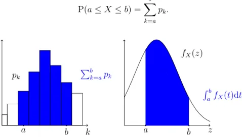
Proposition 3.8 (Calculating probabilities using the distribution). Let X be a discrete random variable with distribution p_k, and let a < b are integers. Then

P(a≤X ≤b) =

b

X

k=a

p_k, P(a≤X) =

∞

X

k=a

p_k,

P(X ≤b) =

b

X

k=−∞

p_k.

Definition 3.9 (Independence of discrete random variables). The discrete random variables X and Y are called independent if for any x∈Z and y∈Z, the events {X =x}

and {Y =y} are independent.

Further readings:

• https://en.wikipedia.org/wiki/Cardinality

• https://www.wolframalpha.com/input/?i=histogram

(27)

3.1 Exercises

Problem 3.1. Let’s consider the probability space related to rolling two dice. Find the distribution of the following discrete random variables.

(a) X := the number shown on the first dice, (b) Y := the number shown on the second dice,

(c) X+Y, (d) max{X, Y},

(e) min{X, Y}, (f) (X−Y)²

Problem 3.2. We take a dice and change the numbers 2 and 3 to show 5. What is the distribution of a number generated by rolling this modified dice?

Problem 3.3. We toss a coin 20 times. What is the distribution of the number of tails shown?

Problem 3.4. Three friends, Chandler, Joey and Ross order 3 different pizzas. When the pizzas are delivered, they are handed out randomly between the three Friends. Denote by X the number of the Friends, who get the pizza they want. What is the distribution of X?

Problem 3.5. A bag contains 5 green and 7 yellow balls. We pull a ball out of the bag, note its colour and put them back. We repeat this process 5 times. Find the distribution of the number of yellow balls drawn. Would it change anything if we didn’t put the balls back in to the bag?

Problem 3.6. We toss a coin. If the result is heads, then we toss the coin once more, else we toss the coin two more times. Denote by X the number of heads shown. What is the distribution of X?

Problem 3.7. There are 3 machines in a factory, which are working at a given time with probability 0.5, 0.6 and 0.7, respectively. Denote by X the number of working machines.

What is the distribution of X?

Problem 3.8. We play the following game. We roll the dice, and if the result is greater than 3, we win HUF 1,000. Furthermore, we can roll the dice again. If the result of the second rolling is greater than 4, we win HUF 2,000, additionally, and we can roll again. If the result of the third rolling is 6, we win HUF 6,000, additionally, and the game is over.

Denote by X the amount of money earned. What is the distribution ofX?

(28)

4 Discrete random variables II. - expectation, notable distributions

In this part we define some special or notable distributions. After that we investigate a crucial object called expectation.

Notable discrete distributions

Definition 4.1 (Bernoulli distribution). Let us consider a random experiment, let A be an event whose probability is P(A) =p, and let

I_A:=

(1, if A happens, 0, otherwise.

Then I_A is the indicator of the event A, it has range {0,1}, and p₀ = P(I_A= 0) = 1−p, p₁ = P(I_A= 1) =p.

Introduce the notation I_A ∼ Bernoulli(p) for the Bernoulli distribution with parameter p.

Example 4.2 (Motivational example: number of successes out of a fixed number of repetitions). Let’s consider the random experiment of rolling a fair dice. Let n∈N be fixed, and repeat the experiment n times independently. Let X denote the number of dices showing 3 or 5. Find the distribution of this discrete random variable.

Answer: The variable X can take the following values: 0,1, . . . , n−1, n. Its distribution is

P(X=k) =

n k

2^k4^n−k

6ⁿ =

n k

2 6

k 4 6

n−k

= n

k 2 6

k 1− 2

6 n−k

for any k ∈ {0,1, . . . , n}.

Definition 4.3 (Binomial distribution). Let us consider a random experiment, and let A be an event whose probability is P(A) = p. Repeat the random experiment n times independently, then let X be the number of times the event A occured. Then X has binomial distribution with parameters n and p and

p_k= P(X =k) = n

k

p^k(1−p)^n−k, k ∈ {0,1, . . . , n}.

Introduce the notation X ∼ binom(n, p) for the binomial distribution with parameters n and p.

Hence we can observe, that the binomial distribution describes the probability of k successes in n draws with replacement, or sampling with replacement. We are drawing with replacement, so it is good to see, that the draws are independent. Another remark is the connection between the binomial and the Bernoulli distribution. We can see, that if X is a binomial distributed variable with parameters n and p, than it has the following representation

X =I₁+· · ·+I_n,

where I_i is the indicator of the event that theith draw is a success, hence I_i ∼Bernoulli(p), i= 1, . . . , n, and these random variables are independent.

(29)

Example 4.4. We have to take a test that consists of 10 questions, where you have to choose between 4 possible answers. Only one of the answers is correct. Suppose we fill out the test randomly. We get the best grade if we answer at least 9 questions correctly, what is the probability of that?

Answer: Let X denote the number of correct answers. Then X has the binomial distribution with parameters n = 10 and p= 0.25, that is

P(X =k) = 10

k

0.25^k0.75^10−k, k ∈ {0,1, . . . ,10}.

Using this formula we get

P(we get the best grade) = P(X ≥9) = P(X = 9) + P(X = 10)

= 10

9

0.25⁹0.75 + 10

10

0.25¹⁰0.75⁰

≈0.0000296.

Example 4.5 (Motivational example: sampling without replacement). Let’s consider the following random experiment. We have a bag with 5 green and 7 red balls and pull 3 balls out. Let X denote the number of green balls drawn. Find the distribution of this discrete random variable.

Answer: The variable X can take the following values: 0,1,2,3. Its distribution is P(X =k) =

5 k

₇

3−k

12 3

, k ∈ {0,1,2,3}.

Definition 4.6 (Hypergeometric distribution). Let us consider the following random experiment. We have a bag withN balls, K green andN−K red balls and pull n balls out.

Let X denote the number of green balls drawn. Then X has hypergeometric distribution with parameters N, K, n and

P(X =k) =

K k

N−K n−k

N n

, k∈ {0,1, . . . , n}.

Introduce the notation X ∼hypergeo(N, K, n) for the hypergeometric distribution with parameters N, K, n.

That is, the hypergeometric distribution describes the probability of k successes in n draws withoutreplacement, orsampling without replacement. The draws are not independent in this case. However, we have the representation

(30)

Example 4.7. We fill out a lottery ticket (5-of-90 lottery). Let X denote the number of correctly guessed numbers. Find the distribution of this discrete random variable. What is the probability of winning some money?

Answer: X has hypergeometric distribution with parameters N = 90, K = 5 and n= 5, that is

P(X =k) =

5 k

₈₅

5−k

90 5

, k ∈ {0,1,2,3,4,5}.

P(winnig some money) = P(X ≥2) = 1−P(X <2) = 1− P(X = 0) + P(X = 1)

= 1−

5 0

₈₅

5

90 5

+

5 1

₈₅

4

90 5

!

≈1−(0.7464 + 0.2304) = 0.0232.

Example 4.8 (Motivational example: number of repetitions until the first success). Let’s consider the random experiment of rolling a fair dice. Let X denote the number of times we have to roll the dice until we see 3 or 5 as the result. Find the distribution of this discrete random variable.

Answer: The random variableX can take any positive integer as a value. Its distribution is

P(X =k) = 4^k−1 6^k =

4 6

^k−1 2 6

for any k ∈N={1,2,3, . . .}.

Definition 4.9 (Geometric distribution). Let us consider a random experiment, and let A be an event whose probability is P(A) =p. Repeat the random experiment until the first occurrence of A and let X be the number of repetitions necessary.

Then X has geometric distributionwith parameter p and

p_k := P(X =k) = (1−p)^k−1p, k ∈N={1,2,3, . . .}.

Introduce the notation X ∼geom(p) for the geometric distribution with parameter p.

This is our first distribution, which has infinite many possible values. We can check that this distribution is well-defined, namely the equation

∞

X

k=1

p_k = 1

holds or not? (See, Theorem 3.5.) To answer this question we need the following results.

Proposition 4.10 (Geometric series). For any p∈(0,1), we have

∞

X

k=0

p^k= 1 1−p. If we use this result, we get

∞

X

k=1

p_k =

∞

X

k=1

(1−p)^k−1p=p

∞

X

k=1

(1−p)^k−1 =p

∞

X

l=0

(1−p)^l =p 1

1−(1−p) = 1, hence the geometric distribution is a well-defined distribution.

(31)

Example 4.11. We play darts. The chance of us hitting the bullseye (the center of the target, that is worth 50 points) is 5%. We keep trying until we hit it. What is the probability of us succeeding in at most 2 tries?

Answer: Let X denote the number of attempts we need. Then X has a geometric distribution with parameter p= 0.05, that is

P(X =k) = 0.95^k−10.05, k ∈ {1,2, . . .}.

Using this formula we get

P(we need at most 2 tries) = P(X ≤2)

= P(X = 1) + P(X = 2)

= 0.05 + 0.95·0.05

= 0.0975.

Expectation of a discrete random variable

In this part our aim is to introduce our first descriptive quantity about a random variable, namely the expectation or mean. We will do so by examining a motivating example.

Example 4.12 (Motivational example). Alice and Bob play the following game. Alice rolls a dice and Bob pays AliceX$, where X is the number shown on the dice. How much should Alice pay Bob for a chance to play this game?

Answer: In each round Alice gets somewhere between 1$ and 6$ from Bob. Clearly if Alice pays less than 1$ per game, then she wins some amount of money each round, while if she pays more than 6$, then she loses some money every round. So the fair price of this game is somewhere between 1$ and 6$.

We can apply the following idea: let Alice play n games and find her average gain, if this average has a limit as n → ∞ then let that be the fair price of the game. Let X, X₁, X₂, . . . , X_n denote independent dice rolls. Then Alice’s average gain after n games is

An := X₁+· · ·+X_n

n = 1

n

X

i=1

Xi.

We can regroup these games by the amount of money Bob has paid in them and get that Alice’s average gain is

A_n = 1 n

6

X

k=1

kk_n(X =k) =

6

X

k=1

kk_n(X =k)

n =

6

X

k=1

kr_n(X =k),

where r_n(X =k) is the relative frequency of the event, that the dice shows k. We would like to interpret the probability of an event by the limit of relative frequencies so ifA_nhas a limit then it is

(32)

Definition 4.13 (Expectation of a discrete random variable). LetX be a discrete random variable with distribution p_k = P(X =k). If the sum

E(X) :=X

k∈Z

k pk

exists, then we call it the expectation (or mean) of X.

There are random variables for which the expectation is not defined, since it can happen that P

k∈Z|k|p_k = ∞. However, if a discrete random variable X is bounded, then its expectation always exists and is finite.

Example 4.14 (Dice roll). Let X denote the result of a fair dice roll. Find E(X).

Answer: The distribution of X is

k 1 2 3 4 5 6

P(X =k) 1/6 1/6 1/6 1/6 1/6 1/6 Hence the expectation of X is

E(X) = 1· 1

6+ 2·1

6 + 3· 1

6 + 4· 1

6+ 5· 1

6+ 6·1

6 = 3.5.

Indeed, this is the same as in the motivational example above.

The expectation of a random variable is a number that indicates the expected or averaged value of the random variable. It means that if we take a lot of independent copies of the random variable, then the average of these numbers oscillates around some number, which is the expectation. This is the so–called law of large numbers.

Theorem 4.15 (Kolmogorov’s strong law of large numbers (1933)). Let X₁, X₂, . . . be independent and identically distributed random variables whose first absolute moment is finite, that is, E(|X1|)<∞. Then

P

n→∞lim

X₁+· · ·+X_n

n = E(X)

= 1.

Thus the law of large numbers means that the average of the independent results of some experiment equals to the expectation. That is the heuristic meaning of the expectation.

Furthermore, we can use the law of large numbers to prove our initial goal, that is to show that the relative frequencies of an event converge to the probability of the same event.

Theorem 4.16 (Law of large numbers and relative frequency). The relative frequency of an event converges to the probability of the event in question with probability 1.

Proof. Indeed, let (Ω,A,P) be a probability space, A ∈ A an event whose probability is P(A) =p∈[0,1]. Repeat the experiment, related to the event A, n times independently and let

I_k:=

(1, if A happens during the k-th repetition, 0, otherwise,

where k ∈ {1, . . . , n}. Then the relative frequency of the event A after n repetitions is the average of the random variables I₁, . . . , I_n, and, by the strong law of large numbers

rn(A) = I1+· · ·+In

n →E(I) =p, n → ∞

holds with probability 1.

Let X be the gain of a game (the amount of money we win). Denote by C the entry fee of the game. In this case the profit is X−C. We have 3 cases.

(33)

• If C = E(X), then the game is fair in the sense that the long-run averaged profit is 0. Hence we can say that E(X) is the fair price of the game.

• If C > E(X), then the game is unfair and it is not favorable to us, because the long-run averaged profit is negative. We should not play this game.

• If C <E(X), then the game is unfair but it is favorable to us, the long-run averaged profit is positive. We should play it.

Proposition 4.17 (Properties of expectation). LetX andY be arbitrary random variables on a probability space (Ω,A,P) whose expectation exists. Then

(i) The expectation is linear, that is for any constants a, b∈R we have E(aX+bY) =aE(X) +bE(Y).

(ii) If the random variables X and Y are independent, then E(XY) = E(X) E(Y).

(iii) Let g :R→R be a function. Then E(g(X)) = X

k∈Z

g(k) P(X =k)

Investigate the expectation of the notable distribution which we already learned.

Theorem 4.18 (Expectation of Bernoulli distribution). Let X ∼Bernoulli(p), then E(X) =p.

Proof: We can use the definition of expectation and get

E(X) = 0·P(X = 0) + 1·P(X = 1) = 0·(1−p) + 1·p=p.

Theorem 4.19 (Expectation of binomial distribution). Let X ∼binom(n, p), then

E(X) =np.

Proof: We can use the definition of expectation and get E(X) =

n

X

k=0

k·P(X =k) =

n

X

k=0

k· n

k

p^k(1−p)^n−k

=np

n

X

n−1 k−1

p^k−1(1−p)^{n−1−(k−1)} =np

m

X m

j

p^j(1−p)^m−j

(34)

However, there is an alternative way to find the expectation of a binomial distribution.

Let X∼binom(n, p), then the distribution of X is the same as the distribution of Y₁+· · ·+Y_n,

where Y_i ∼Bernoulli(p), i=1,. . . ,n.

Using the linearity of the expectation and the expectation of the Bernoulli distribution, we get

E(X) = E(Y₁+· · ·+Y_n) = E(Y₁) +· · ·+ E(Y_n) =np.

Theorem 4.20 (Expectation of geometric distribution). Let X ∼geom(p), then

E(X) = 1 p.

Proof: We can use the definition of expectation and get the result directly. However, as in the case of binomial, there is an alternative way again to find the expectation of the geometric distribution. We have to ask the question what if we fail or succeed on the first trial?

We succeed with probability p and if we do then X = 1. If we fail (with probability 1−p), then we can denote the remaining trials until the first success by Y. Note that Y has the same distribution as X and therefore has the same expectation. We arrive at the following equation

E(X) = pE(1) + (1−p) E(1 +Y) = p+ (1−p) E(1 +X)

=p+ (1−p)(1 + E(X)) = 1 + (1−p) E(X) Hence

E(X)−(1−p) E(X) = 1 E(X) = 1

p.

For the precise proof, see the remark after Proposition 6.12

Theorem 4.21 (Expectation of hypergeometric distribution). LetX ∼hypergeo(N, K, n), then

E(X) =nK N.

Proof: For the proof, as in the binomial and the geometric case as well, we have two possibilities. One can use some combinatorial identities, and then after some tedious calculations, the result can be derived.

The other way is similar as in the binomial case. The distribution of X is the same as the distribution of

Y1+· · ·+Yn,

whereY_i ∼Bernoulli(p_i), i=1,. . . ,n, namelyY_i is the result of theith trial. It can be shown (we will see it when we learn about conditional probability, see Example 6.10), that the distributions ofY_i are the same, andp_i = ^K_N. That is, using the linearity of the expectation and the expectation of the Bernoulli distribution, we get

E(X) = E(Y₁+· · ·+Y_n) = E(Y₁) +· · ·+ E(Y_n) = nK N.

(35)

Further readings:

• https://en.wikipedia.org/wiki/List_of_probability_distributions

• https://en.wikipedia.org/wiki/Expected_value

• https://en.wikipedia.org/wiki/Law_of_large_numbers

• https://en.wikipedia.org/wiki/Geometric_series

(36)

4.1 Exercises

Problem 4.1. We get 6 lottery tickets as a birthday present; each ticket has a 40%

probability of winning. What is the probability that we will have exactly 4 winning tickets?

What is the expected number of winning tickets?

Problem 4.2. At a fair, we can play the following game: we throw a coin until we obtain heads, then we get 100 Ft times the number of throws. How much should we pay to play this game?

Problem 4.3. At a driving test, we pass with a probability of 15% each time. Each test costs HUF 10,000. What is the probability that we will pass the test exactly on the fifth try? What is the expected cost of the tests if we keep trying until we obtain a driver’s license?

Problem 4.4. On a city road there are 5 traffic lights. If we have to stop for a light, we lose 10 seconds. Supposing that the lamps operate independently of each other and that there is a 60% chance of having to stop for a light, what is the expected amount of delay on this road? What is the probability that we will be delayed exactly 30 seconds?

Problem 4.5. We throw two dices simultaneously. If the sum of the numbers is 3, we get HUF 100, if the sum is 7, we get HUF 30. How much should we pay to play this game?

Problem 4.6. In the 5-of-90 lottery the winnings are: 500,000,000 for 5 hits, 2,000,000 for 4 hits, 300,000 for 3 hits and 2,000 for 2 hits. What is the expectation of our winnings?

Problem 4.7. We can play the following game. We roll with a dice once and we can find the amount of money we win in this table.

result 1 2 3 4 5 6

prize 0 0 0 250 250 1000 What is the fair price for this game?

Problem 4.8. We can play the following game. We roll with a dice three times and we win HUF 54,000 if we roll only sixes, otherwise we win nothing. What is the fair price for this game?

Problem 4.9. In a video game there is a very difficult map. We only have 0.17 probability of completing the map successfully. If we fail the map, we can try again as many times as we wish. Each attempt takes 10 minutes. What is the expected number of attempts needed to complete the map? What is the expected time to finish the map? We only have an hour to play, what is the chance of success during that time?

Problem 4.10. We run a cinema, tonight is the premier of the new Star Wars movie, and we sold all 100 tickets. However we have a problem. We only have enough popcorn for 35 servings. Assume that each person buys popcorn for the movie with a probability 0.2 independently of each other. What is the probability that everyone gets popcorn who wants to buy it?

Problem 4.11. We toss a fair coin 3 times. If all tosses result in the same outcome, then we have to pay HUF 32 , if we get exactly 2 heads, we win HUF 64 and finally if we get exactly 2 tails we win HUF 16. What is the fair price of this game? How would this price change if we would exchange our fair coin with a biased one, that lands on heads only 1/4 of the time?

(37)

Problem 4.12. * A drunk sailor comes out of a pub. He is so drunk that every minute he picks a random direction (up the street or down the street) with equal probability. What is the probability that he will be back at the pub after 10 minutes? What is the probability of coming back after 20 minutes? What if he prefers to go up the street with probability 2/3?

Problem 4.13. * (Coupon collector’s problem) The Leays company comes up with the following promotion. They put a card with one of the following colours into every bag of chips: red, yellow, blue, purple, green. Anyone who collects a card of each colour gets a mug with the Leays logo on it for free. The company hires us to investigate the effects of this promotion. What is the expected number of chips someone has to buy to collect one of each card? (Assume that a bag of chips contains any of the coloured cards with equal probability.)