3 Light curve

Volume 63 Number 6263 DOI: 10.22444/IBVS.6263

Konkoly Observatory Budapest

27 March 2019 HU ISSN 0374 – 0676

ON THE PERIOD AND LIGHT CURVE OF THE A-TYPE W UMa BINARY GSC 3208 1986

EATON, JOEL A.¹; ODELL, ANDREW P.²; POLAKIS, THOMAS A.³

17050 Bakerville Road, Waverly, TN 37185 USA; e-mail: eatonjoel@yahoo.com

2Dept of Physics and Astronomy, NAU Box 6010, Flagstaff AZ 86011 USA; e-mail: WCorvi@yahoo.com

3Command Module Observatory, 121 W. Alameda Dr., Tempe, AZ 85282 USA; e-mail: tpolakis@cox.net Abstract

We present a new period study and light-curve solutions for the A-Type W UMa binary GSC 3208 1986. Contrary to a previous claim by R. G. Samec et al. of a rapidly decreasing period, the system’s period is increasing moderately on a timescale of 2×10⁶ years. The light curve is variable on the time scale of years, which can be understood by changes in how much it overfills its Roche lobe.

Contact binaries are binaries close enough that their components are enclosed in a common, probably convective envelope (Lucy 1968). The best known members of this class are the W Ursae Majoris systems (Binnendijk 1970), although there are other rarer binaries that may be in marginal contact (e.g., Ka lu˙zny 1983, 1986a–d; Siwak et al.

2010). Binnendijk (pp. 218-221) defined two varieties of these W UMa systems, A-types, with transit primary eclipses, and W-types, with occultation primaries. Given the direct dependence of the ratio of radii on mass ratio in contact binaries, these A- and W-type classes correspond to q=M²/M¹ less than and greater than 1.0, respectively.

GSC 3308 1986 (α(2000)=22^h25^m16.^s0,δ(2000)=+41^◦27^′51.^′′9) is a faint A-type W UMa binary observed and analyzed by Samec et al. (2015a; hereafter ^SAMEC). ^SAMECobtained four nights of photometry (σB≈0.006) and found an F3 V spectral type from a spectrum taken at the Dominion Astrophysical Observatory, a mass ratio of q=0.24, and that the star overfills its Roche lobe by 39%. These properties are not surprising for such a system, butSAMECalso derived a very rapid perioddecrease, corresponding to a timescale of 3×10⁵ years. This seems unlikely for what they claim is an “ancient” contact system, especially if caused by magnetic braking, their favored period-change mechanism.

1 Ephemeris

Suspecting that the radical period decrease might result from R. G. Samec’s previously documented (Odell et al. 2011) error of confusing Modified Julian Date (Heliocentric Julian Date – 2,400,000.5) with Reduced Julian Date (HJD – 2,400,000.0) in data from the Northern Sky Variability Survey (NSVS, see Wozniak et al. 2004), we obtained the archival data from the NSVS and SuperWASP (SWASP, see Butters et al. 2010) web sites.

We have subsequently obtained new light curves for 2017 and 2018 (Polakis;BVRI on the

2 IBVS6263

UBV/Cousins system; Table 1, provided as online table 6263-t1.txt at the IBVS web site) and added the published photometry of Liakos & Niarchos (2011) and^SAMECto give nine seasonal light curves. Using these, we find a very different result than ^SAMEC. We have derived new effective times of minimum for these nine epochs by fitting those seasonal light curves with the Wilson-Devinney code to measure phase shifts with respect to the ephemeris of Eq. 1. These are listed in Table 2; the errors given are theσ’s calculated by the W–D code multiplied by a factor of three per Popper (1984).

Table 2. O–C Residuals for linear and quadratic elements (days).

Epoch (Obs) Cycle (Obs–Calc) (Obs–Calc) Source of data

RJD (N) linear quadratic

(Eq. 1) (Eq. 2)

51464.1096 ± 0.0010 -11693 0.0022 -0.0017 NSVS

53247.4351 ± 0.0003 -7285 -0.0005 0.0003 SWASP 2004 53989.8134 ± 0.0006 -5450 -0.0014 0.0003 SWASP 2006

54324.7939 ± 0.00011 -4622 -0.0018 0.0000 SWASP 2007 Epoch1 54374.1509 ± 0.00013 -4500 -0.0019 -0.0001 SWASP 2007 Epoch2 55410.2457 ± 0.0005 -1939 -0.0013 -0.0001 Liakos&Niarchos 56194.7011 ± 0.0003 0 0.0000 -0.0001 Samec

57925.8458 ± 0.0003 4279 0.0055 -0.0003 Polakis 2017 58415.7787 ± 0.0002 5490 0.0081 0.0001 Polakis 2018

In analyzing the period, we first used a preliminary linear ephemeris derived by Odell from the NSVS plus Polakis’ 2017 data, namely

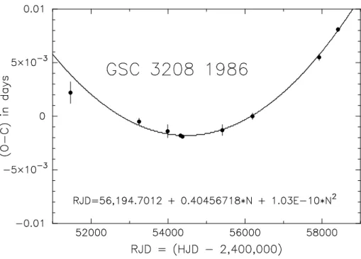
HJD Tmin I = 2,456,194.7011 + 0.4045663×N, (1) to phase all the data into annual/seasonal light curves. Then we derived the deviations of the phases from this linear ephemeris with the W-D code as noted above, and then fit those deviations with a second-order polynomial to determine the following quadratic ephemeris:

HJD Tmin I = 2,456,194.7012(1) + 0.40456718(1)×N + 1.03(5)×10⁻¹⁰×N². (2) In this equation the numbers in parentheses are errors in the last decimal place, and N is the cycle number. Fig. 1 shows the deviations from Eq. 1 and the quadratic fit.

2 Spectra

Odell obtained two spectra of GSC 3208 1986 with the Boller&Chivens Spectrograph on the Steward Observatory 90-inch telescope around 1 June 2015, specifically at HJD 2,457,173.9734 (phase 0.55) and HJD 2,457,174.8694 (phase 0.76). These spectra covered the wavelength range 3900–4750 ˚A and are consistent with the F3 V spectral type of

SAMEC. They give radial velocities for the components of RV1 = 22.1±7.2 km s⁻¹ for the phase near conjunction and RV1 = 86.9±8.2 km s⁻¹ and RV2 = −298±25 km s⁻¹ for the quadrature. These values give a crude indication of the velocity amplitudes of the components, K1 = 91±16 km s⁻¹ and K2 = 294±25 km s⁻¹ with γ = −4 km s⁻¹. The resulting spectroscopic mass ratio q = 0.30±0.03 is ∼ consistent with the photometric mass ratio.

Figure 1. O–C Diagram for GSC 3208 1986.

3 Light curve

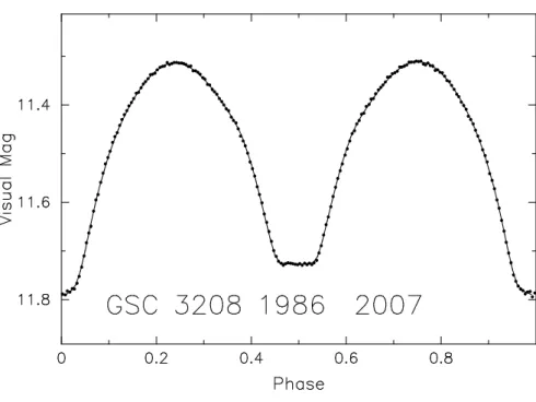
The extensive observations from SWASP give us the opportunity to solve well-defined light curves for the three years, 2007, 2006, and 2004. The data for 2007 are by far the best and most numerous, so we will concentrate on them. Consequently, we have formed 200 normal points derived from the roughly 11,300 SWASP observations for 2007, giving them in online Table 3 (available through the IBVS website as 6263-t3.txt) as orbital phase (based on Eq. 1), magnitude, and a standard deviation of the mean for each magnitude. The typical normal point has an uncertainty of σ= 0.0019 mag (S.D.), nominally giving about the same total weight as the photometry published by^SAMEC, but the SWASP data cover enough time to average out the typical wavelength-independent observational errors of data taken on a mere four nights. These data represent a broad band in the optical, corresponding roughly to V of the UBV system. Fig. 2 shows the SWASP light curves for 2007 (Table 3) with a representation of the solution of Table 4 plotted as a solid line.

We have solved this light curve with the Wilson-Devinney code [2003 version; see Wilson & Devinney (1971); Wilson (1990,94)], finding the elements in the second col- umn of Table 4. These are roughly consistent with ^SAMEC’s solution (Table 4, Col. 4).

In calculating this solution we adopted ^SAMEC’s temperature of the primary, convective gravity darkening (Lucy 1967), convective reflection effect (Rucinski 1969), the Kurucz- atmospheres option in the W-D code, and a linear limb-darkening coefficient from Van Hamme (1993). We accounted for a slight O’Connell effect in the normal points with a small dark spot on the leading hemisphere of the primary component. The small χ² indi- cates the model fits the data as well as can be expected. For completeness, we calculated a solution for 2007 with radiative gravity darkening and reflection effect, because in the past there was some inkling that these hotter A-type systems might be radiative, but the fit was much worse, by a factor of two in χ². This radiative solution had a significantly lower fillout, 13%, as expected from the well-known correlation between fillout and gravity

4 IBVS6263

Figure 2. Light curve solution for SWASP, normal points for 2007.

darkening.

The other two years of SWASP data had somewhat different light curves which we have solved by varying those elements of the 2007 solution that might conceivably change on the timescale of a few years. Some elements, such asqand i, cannot change materially on such a short timescale, so we are left with temperatures and fillout that might change.

Keeping q, i,T1 fixed, we get the solution in Col. 3 of Table 4 for 2004. A greater depth of both eclipses in 2004 led to a larger overfilling of the Roche lobe. The solution for 2006 had a marginally larger fillout, 39%, for the worst data of the three years (σ = 0.014 mag). The differences between 2007 and 2004 might conceivably result from a change in the photometric band of the observations, but it would require a shift at least as great as from V to B between the two years. A shift of this magnitude is rather unlikely (see Butters et al. 2010, Fig. 1).

All of these solutions imply that the standard overcontact model fits GSC 3208 1986 well. Values of Tmult, which measures the ratio of T2 as measured in W-D, Mode 3, to its value for W-D, Mode 1, (no break in temperature at the neck between the components), are 1.0 for all practical purposes, so the temperature varies smoothly over the surface as determined by the gravity-darkening law. The solution for a radiative envelope, however, does not have this property and gives a significantly worse fit, so the envelope is not likely to be radiative.

You may have noticed that the quoted errors of our solution for 2007 and SAMEC’s solution for 2012 are inconsistent, although the two data sets have roughly the same weight (#points/σ²). This probably results from the way such uncertainties are calculated. If we calculate the uncertainty of each element independently of all the others, we get values for the 2007 SWASP solution similar to those quoted by SAMEC. However, if we let elements q, i, Ω, T2, and the x’s vary simultaneously, we get the uncertainties listed. Adding g and Abol to the mix gives even bigger uncertainties, doubling the reported uncertainty of Ω. This result confirms Popper’s (1984) insinuation that the uncertainties derived by the

Table 4. GSC 3208 1986: Light curve solutions

Parameter 2007-SWASP 2004-SWASP 2012-SAMEC 2017-Polakis 2018-Polakis

(1) (2) (3) (4) (5) (6)

x1=x2(fixed) 0.51 0.51 Non-linear 0.63,0.51,0.41,0.33 0.63,0.51,0.41,0.33

g(fixed) 0.32 0.32 0.32 0.32 0.32

A_bol(fixed) 0.50 0.50 0.50 0.50 0.50

i(deg) 85.60±0.27 85.60 (fixed) 85.8±0.1 85.60 (fixed) 85.60 (fixed) q(M2/M1) 0.2424±0.0011 0.2424 (fixed) 0.2374±0.0002 0.2424 (fixed) 0.2424 (fixed) Ω 2.2811±0.0020 2.269±0.0020 2.261±0.001 2.273±0.0018 2.279±0.0016

fillout 35.3 ±1.3% 49.1±1.3% 39±0.7% 40.3±1.2% 36.8±1.0%

T1 (K, fixed) 6875 6875 6875 6875 6875

T2 (K) 6757±22 6789±10 6760±? 6745±11 6725 ±8

Tmult 0.9950±0.0032 1.0009±0.0014 0.9968 0.9948 0.9909

σ(mag) 0.0019/point 0.0066/point ∼0.006/point ∼0.013/point ∼0.013/point

χ²/DOF 1.2 1.1 ∼1.44 ∼2.2 ∼1.0

Spot on the Primary Component

lat,long (deg) 0,270 0,270 none none none

rspot(deg) 1.7 1.7

Tspot (black) (black)

W-D code are misleading. It also points to the intuitive truth that our assumptions about limb darkening, gravity darkening, and reflection effect will inevitably bias the results for all these contact and near-contact binaries.

Acknowledgements: We thank Steward Observatory for allocating the telescope time to obtain the spectra we used. This paper makes use of data from the Data Release 1 of the WASP data (Butters et al. 2010) as provided by the WASP consor- tium, and the computing and storage facilities at the CERIT Scientific Cloud, reg. no.

CZ.1.05/3.2.00/08.0144, which is operated by Masaryk University, Czech Republic. It also uses data from the Northern Sky Variability Survey created jointly by the Los Alamos National Laboratory and University of Michigan.

References:

Binnendijk, L., 1970, ARA&Ap, 12, 217 DOI

Butters, O. W. et al., 2010, A&A 520, L10 (SuperWASP) Ka lu˙zny, J., 1983,AcA, 33, 345

Ka lu˙zny, J., 1986a, AcA, 36, 105 Ka lu˙zny, J., 1986b, AcA, 36, 113 Ka lu˙zny, J., 1986c, AcA, 36, 121 Ka lu˙zny, J., 1986d, PASP, 98, 662

Liakos, A., Niarchos, P., 2011, IBVS, 5999, 2 Lucy, L. B., 1967, ZsfAp, 65, 89

Lucy, L. B., 1968, ApJ, 151, 1123 DOI

Odell, A.P., Wils, P., Dirks, C., Guvenen, B., O’Malley, C.J., Villarreal, A.S., Weinzettle, R.M., 2011, IBVS, 6001

Popper, D. M., 1984,AJ, 89, 132 DOI Rucinski, S.M., 1969, AcA, 19, 245

6 IBVS6263

Samec, R. G., Kring, J. D., Robb, R., Van Hamme, W., Faulkner, D. R., 2015a,AJ,149, 90 (^SAMEC) DOI

Samec, R. G., Benkendorf, B., Dignan, J. B., Robb, R., Kring, J., Faulkner, D. R., 2015b, AJ,149, 146 DOI

Siwak, M., Zola, S., Koziel-Wierzbowska, D., 2010,AcA, 60, 305 Van Hamme, W., 1993,AJ,106, 2096 DOI

Wilson, R.E., Devinney, E.J., 1971, ApJ, 166, 605 DOI Wilson, R. E., 1990, ApJ, 356, 613 DOI

Wilson, R. E., 1994, PASP, 106, 921 DOI

Wozniak, P. R. et al., 2004, AJ, 127, 2436 (NSVS) DOI