Tools for discovering and characterizing extrasolar planets PhD Dissertation

(1)

Tools for discovering and characterizing extrasolar planets

PhD Dissertation

Written by: Andr´ as P´ al

Loránd Eötvös University, Faculty of Sciences PhD School of Physics

PhD Program of Particle- and Astrophysics

Head of PhD School of Physics: Prof. Zal´an Horv´ath Head of the PhD program: Prof. Ferenc Csikor

Thesis advisor: Dr. G´asp´ar Bakos,

postdoctoral fellow of the National Science Foundation Harvard-Smithsonian Center for Astrophysics

Supervisor: Prof. Bálint ´ Erdi, professor Department of Astronomy Loránd Eötvös University

Loránd Eötvös University Budapest, Hungary

2009

(2)

(3)

Foreword

Among the group of extrasolar planets, transiting planets provide a great opportunity to obtain direct measurements for the basic physical properties, such as mass and radius of these objects. These planets are therefore highly important in the understanding of the evolution and formation of planetary systems: from the observations of photometric transits, the interior structure of the planet and atmospheric properties can also be constrained. The most efficient way to search for transiting extrasolar planets is based on wide-field surveys by hunting for short and shallow periodic dips in light curves covering quite long time intervals. These surveys monitor fields with several degrees in diameter and tens or hundreds of thousands of objects simultaneously. In the practice of astronomical observations, surveys of large field-of-view are rather new and therefore require special methods for photometric data reduction that have not been used before. Since 2004, I participate in the HATNet project, one of the leading initiatives in the competitive search for transiting planets. Due to the lack of software solution which is capable to handle and properly reduce the yield of such a wide-field survey, I have started to develop a new package designed to perform the related data processing and analysis. After several years of improvement, the software package became sufficiently robust and played a key role in the discovery of several transiting planets.

In addition, various new algorithms for data reduction had to be developed, implemented and tested which were relevant during the reduction and the interpretation of data.

In this PhD thesis, I summarize my efforts related to the development of a complete software solution for high precision photometric reduction of astronomical images. I also demonstrate the role of this newly developed package and the related algorithms in the case of particular discoveries of the HATNet project.

(4)

(5)

Chapter 1 Introduction

In the last two decades, the discovery and characterization of extrasolar planets became an exciting field of astronomy. The first companion that was thought to be an object roughly 10 times more massive than Earth, had been detected around the pulsar PSR1829-10 (Bailes, Lyne & Shemar, 1991). Although this detection turned out to be a false one (Lyne & Bailes, 1992), shortly after the method of detecting planetary companions involving the analysis of pulsar timing variations led to the successful confirmation of the multiple planetary system around PSR1257+12 (Wolszczan & Frail, 1992). The pioneering discovery of a planet orbiting a main sequence star was announced by Mayor & Queloz (1995). They reported the presence of a short-period planet orbiting the Sun-like star 51 Peg. This detection was based on precise radial velocity measurements with uncertainties at the level of meter per second. Both discovery methods mentioned above are based on the fact that all components in a single or multiple planetary system, including the host star itself, revolve around the common barycenter, that is the point in the system having inertial motion. Thus, companions with smaller masses offset the barycenter only slightly from the host star whose motion is detected, either by the analysis of pulsar timing variations or by radial velocity measurements. Therefore, such methods – which are otherwise fairly common among the investigation techniques of binary or multiple stellar systems – yielded success in the form of confirming planets only after the evolution of instrumentation. Due to the physical con- straints found in these methods, the masses of the planets can only be constrained by a lower limit, while we even do not have any information on the sizes of these objects.

The discovery of 51 Peg b was followed by numerous other detections, mainly by the method of radial velocity analysis, yielding the discovery, for instance, of the first planetary system with two planets around 47 UMa (Butler & Marcy, 1996; Fischer et al., 2002), and the first multiple planetary system around υ And (Butler et al., 1999). Until the first photometric detection of planetary transits in the system of HD 209458(b) (Henry et al., 2000; Charbonneau et al., 2000), no radius estimations could be given to the detected

(10)

planets, and all of these had only lower limits for their masses. Transiting planets provide the opportunity to characterize the size of the planet, and by the known inclination of its orbit, one can derive the mass of the planet without any ambiguity by combining the results of transit photometry with the radial velocity measurements. The planetary nature of HD 209458b was first confirmed by the analysis of radial velocity variations alone. The first discovery based on photometric detection of periodic dips in light curves was the discovery of OGLE-TR-56b (Konacki et al., 2003). Since several scenarios can mimic events that have similar light curves to transiting planets, confirmation spectroscopy and subsequent analysis of radial velocity data is still necessary to verify the planetary nature of objects found by transit searches (Queloz et al., 2001; Torres et al., 2005).

Since the first identification of planetary objects transiting their parent stars, numerous additional systems have been discovered either by the detection of transits after a confirmation based on radial velocity measurements or by searching transit-like signals in photometric time series and confirming the planetary nature with follow-up spectroscopic and radial velocity data. The former method led to the discovery of transits for many well-studied systems, such as HD 189733 (planet transiting a nearby K dwarf; Bouchy et al., 2005), GJ 436 (Butler et al., 2004), HD 17156 (Fischer et al., 2007; Barbieri et al., 2007) or HD 80606 (the transiting planet with the longest known orbital period of∼111 days; Naef et al., 2001; Moutou et al., 2009). These planets with transits confirmed later on are found around brighter stars since surveys for radial velocity variations mainly focus on these. However, the vast major- ity of the currently known transiting extrasolar planets have been detected by systematic photometric surveys, fully or partially dedicated for planet searches. Such projects monitor either faint targets using telescopes with small field-of-view or bright targets involving large field-of-view optical instrumentation. Some of the projects focused on the monitoring of smaller fields are the Monitor project (Irwin et al., 2006; Aigrainet et al., 2007), Deep MMT Transit Survey (Hartman et al., 2008), a survey for planetary transits in the field of NGC 7789 by Bramich et al. (2005), the “Survey for Transiting Extrasolar Planets in Stellar Systems” by Burke et al. (2004), “Planets in Stellar Clusters Extensive Search” (Mochejska et al., 2002, 2006), “Single-field transit survey toward the Lupus” of Weldrake et al. (2008), the SWEEPS project (Sahu et al., 2006), and the Optical Gravitational Lensing Experiment (OGLE) (Udalski et al., 1993, 2002; Konacki et al., 2003). Projects monitoring wide fields are the Wide Angle Search for Planets (WASP, SuperWASP, see Street et al., 2003; Pol- lacco et al., 2004; Cameron et al., 2007), the XO project (McCullough et al., 2005, 2006), the Hungarian-made Automated Telescope project (HATNet, Bakos et al., 2002, 2004), the Transatlantic Exoplanet Survey (TrES, Alonso et al., 2004), the Kilodegree Extremely Lit- tle Telescope (KELT, Pepper, Gould & DePoy, 2004; Pepper et al., 2007), and the Berlin Extrasolar Transit Search project (BEST, Rauer et al., 2004). One should mention here the existing space-borne project, theCoRoTmission (Barge et al., 2008) and theKeplermission,

(11)

launched successfully on 7 March 2009 (Borucki et al., 2007). Both missions are dedicated (in part time) to searching for transiting extrasolar planets. As of March 2009, the above mentioned projects announced 57 planets. 6 planets were found by radial velocity surveys where transits were confirmed after the detection of RV variations (GJ 436b, HD 149026b, HD 17156b, HD 80606b, HD 189733b and HD 209458b), while the other 51 were discovered and announced by one of the above mentioned surveys. The CoRoT mission announced 7 planets, for which 4 had published orbital and planetary data; the OGLE project reported data for 7 planets and an additional planet with existing photometry in the OGLE archive has also been confirmed by an independent group (Snellen et al., 2008); the Transatlantic Exoplanet Survey reported the discovery of 4 planets; the XO project has detected and confirmed 5 planets; the SWEEPS project found 2 planets; the SuperWASP project announced 14 + 1 planets, however, 2 of them are known only from conference announcements; and the HATNet project has 10 + 1 confirmed planets. The planet WASP-11/HAT-P-10b had a shared discovery, it was confirmed independently by the SuperWASP and HATNet groups (this common discovery has been denoted earliet by the +1 term). The HATNet project also confirmed independently the planetary nature of the object XO-5b (P´al et al., 2008c).

All of the above mentioned wide-field surveys involve optical designs that yield a field-of- view of several degrees, moreover, the KELT project monitors areas having a size of thousand square degrees (hence the name, “Kilodegree Extremely Little Telescope”). The calibration and data reduction for such surveys revealed various problems that were not present on the image processing of “classical” data (obtained by telescopes with fast focal ratios and therefore smaller field-of-view). Some of the difficulties that occur are the following. Even the calibration frames themselves have to be filtered carefully, in order to avoid any significant structures (such as patches of clouds in the flat field images). Images taken by fast focal ratio optics have significant vignetting, therefore the calibration process should track its side effects, such as the variations in the signal-to-noise level across the image. Moreover, fast focal ratio yields comatic aberration and therefore systematic spatial variations in the stellar profiles. Such variations make the source extraction and star detection algorithms not only more sensitive but also are one of the major sources of the correlated noise (or red noise) presented in the final light curves ¹. Due to the large field-of-view and the numerous individual objects presented in the image, the source identification and the derivation of the proper “plate solution” for these images is also a non-trivial issue. The photometry itself is hardened by the very narrow and therefore undersampled sources. Unless the effects of the undersampled profiles and the spatial motions of the stellar profiles are handled with care, photometric time series are affected by strong systematics. Due to the short fractional duration and the shallow flux decrease of the planetary transits, several thousands of in-

1The time variation of stellar profiles is what causes red noise

(12)

dividual frames with proper photometry are required for significant and reliable detection.

Since hundreds of thousands of stars are monitored simultaneously during the observation of a single field, the image reduction process yields enormous amount of photometric data, i.e. billions of individual photometric measurements. In fact, hundreds of gigabytes up to terabytes of processed images and tabulated data can be associated in a single monitored field. Even the most common operations on such a large amount of data require special methods.

The Hungarian Automated Telescope (HAT) project was initiated by Bohdan Paczýski and Gáspár Bakos (Bakos et al., 2002). Its successor, the Hungarian-made Automated Telescope Network (Bakos et al., 2004) is a network of small class of telescopes with large field-of-view, dedicated to an all-sky variability survey and search for planetary transits. In the past years, the project has became one of the most successful projects in the discovery of almost one fifth of the known transiting extrasolar planets. After joining the project in 2004, the author’s goal was to overcome the above mentioned issues and problems, related to the image processing of the HATNet data. In this thesis, the efforts for the development of a software package and its related applications in the HATNet project are summarized.

This PhD thesis has five chapters. Following the Introduction, the second chapter, “Al- gorithms and Software environment” discusses the newly developed and applied algorithms that form the basis of the photometry pipeline, and gives a description on the primary concepts of the related software package in which these algorithms are implemented. The third chapter, “HATNet discoveries” describes a particular example for the application of the software on the analysis of the HATNet data. This application and the discussion is related to the discovery of the planet HAT-P-7b, transiting a late F star on a quite tight orbit. The fourth chapter, “Follow-up observations” focuses on the post-discovery measurements (including photometric and radial velocity data) of the eccentric transiting exoplanetary system of HAT-P-2b. The goals, methods and theses are summarized in the fifth chapter.

(13)

Chapter 2 Algorithms and Software environment

In principle, data reduction or simply reduction is the process when the raw data obtained by the instrumentation are transformed into a more useful form. In fact, raw data can be analyzed during acquisition in order do modify the instrumentation parameters for the subsequent measurements¹. However, in the practice of astronomical data analysis, all raw data are treated to be known in advance of the reduction process. Moreover, the term “more useful form” of data is highly specific and depends on our needs. Regarding to photometric exoplanetary studies, this “more useful form” means two things. First – as in the case of HATNet where the discoveries are based on long-term photometric time series –, reduction ends at the stage of analyzed light curves, where transit candidates are recovered by the result of this analysis. Second, additional high-precision photometry² yields precise information directly about the planet itself. One should mention here that other types of measurements involving advanced and/or space-borne techniques (for instance, near-infrared photometry of secondary eclipses) have same principles of the reduction. The basics of the reductions are roughly the same and such observations yield even more types of planetary characteristics, such as brightness contrast or surface temperature distribution.

The primary platform for data reduction is computers and the reduction processes are performed by dedicated software systems. As it was mentioned in the introduction, existing software solutions lack several relevant components that are needed for a consistent analysis of the HATNet data flow. One of our goals was to develop a software package that features

1For instance, in the case of HATNet, real-time astrometric guiding is used to tweak the mount coordinates in the cases when the telescope drifts away from the desired celestial position. This guiding basically uses the same algorithms and routines that are involved in the photometric reduction. Like so, simplified forms of photometry can be used in the case of follow-up measurements of exoplanetary candidate host stars: if light curve variations show unexpected signals, the observation schedule could be changed accordingly to save expensive telescope time.

2Combined with additional techniques, such as spectroscopy or stellar evolution modelling. The confirmation the planetary nature by radial velocity measurements is essiential.

(14)

all of the functionality required by the proper reduction of the HATNet and the related follow-up photometry. The package itself is namedfi/fihat, referring to both the HATNet project as well as the invocation of the related individual programs.

In the first major chapter of this PhD thesis, I summarize both the algorithms and their implementations that form the base of thefi/fihatsoftware package. Due to the difficulties of the undersampled and wide-field photometry, several new methods and algorithms should have been developed, tested and implemented that were missing from existing and available image reduction packages. These difficulties are summarized in the next section (Sec. 2.1) while the capabilities and related problems of existing software solutions are discussed in Sec. 2.2.

The following sections describe the details of the algorithms and methods, focusing pri- marily on those that do not have any known implementation in any publicly available and/or commercial software. Sec. 2.3 discusses the details of the calibration process, Sec. 2.4 describes how the point-like sources (stars) are detected, extracted and characterized from the images, the details of the astrometry and the related problems – such as automatic source identification and obtaining the plate solution – are explained in Sec. 2.5, the details of the image registration process is discussed in Sec. 2.6, Sec. 2.7 summarizes the problems related to the instrumental photometry, Sec. 2.8 describes the concepts of the “image subtraction”

process, that is mainly the derivation of a proper convolution transformation between two registered images, Sec. 2.9 explains how can the photometry be optimally performed on convolved or subtracted images. Sec. 2.10 describes the major concepts of how the still remaining systematic light curve variations can be removed.

In Sec. 2.11, after the above listed description of the crucial steps of the whole image reduction and photometry process, I outline the major principles of the newly developed software package. This part is then followed by the detailed description of the individual components of the software package. And finally, the chapter ends with the practices about how this package can be used in order to perform the complete image reduction process.

2.1 Difficulties with undersampled, crowded and wide- field images

In this section we summarize effects that are prominent in the reduction of the HATNet frames when compared to the “classical” style of image reductions. The difficulties can be categorized into three major groups. These groups do represent almost completely different kind of problems, however, all of these are the result of the type of the survey. Namely, these problems are related to theundersampled property, the crowding of the sources that are the point of interest and the large field-of-view of the images. In this section we examine what

(15)

2.1. UNDERSAMPLED, CROWDED AND WIDE-FIELD IMAGES

0.010 0.015 0.020 0.025 0.030 0.035

0.0 0.2 0.4 0.6 0.8 1.0

Light curve RMS

Subpixel-level inhomogenity in the quantum efficiency (Q) FWHM = 1.0

FWHM = 1.1

FWHM = 1.2 FWHM = 1.4

Figure 2.1: Plot showing the light curve scatter (rms, in magnitudes) of a mock star with various FWHMs and having a flux ofI= 10000 (in electrons). The light curve rms is plotted as the function of the subpixel-level inhomogeneity,Q. Supposing a pixel structure where the pixel is divided to two rectangles of the same size,Qis defined as the difference in the normalized quantum efficiencies of these two parts (i.e. Q= 0 represents completely uniform sensitivity and atQ= 1 one of the parts is completely insensitive (that is typical for front-illuminated detector).

particular problems arise due to these properties.

2.1.1 Undersampled images

At a first glance, an image can be considered to be undersampled if the source profiles are

“sharp”. The most prevalent quantity that characterizes the sharpness of the (mostly stellar) profiles is thefull width at half magnitude (FWHM). This parameter is the diameter of the contour that connects the points having the half of the source’s peak intensity. Undersampled images therefore have (stellar) profiles with small FWHM, basically comparable to the pixel size. In the following, we list the most prominent effects of such a “small” FWHM and also check what is the practical limit below which this “small” is really small. In this short section we demonstrate the yields of various effects that are prominent in the photometry for stellar profiles with small FWHMs. All of these effects worsen the quality of the photometry unless special attention is made for their reduction.

Subpixel structure

The effect of the subpixel structure is relevant when the characteristic length of the flux variations becomes comparable to the scale length of the pixel-level sensitivity variations in the CCD detector. The latter is resulted mostly by the presence of the gate electrodes on the surface of the detector, that block the photons at certain regions of a given pixel.

Therefore, this structure not only reduces the quantum efficiency of the chip but the signal depends on the centroid position of the incoming flux: the sharper the profile, the larger the dependence on the centroid positions. As regards to photometry, subpixel structure

(16)

0.00 0.01 0.02 0.03 0.04

1 2 3 4

Light curve RMS

FWHM = 1.0

1 2 3 4

FWHM = 1.5

1 2 3 4

Aperture radius (in pixels) FWHM = 2.2

1 2 3 4

FWHM = 2.7

1 2 3 4

FWHM = 3.3

1 2 3 4

FWHM = 3.9

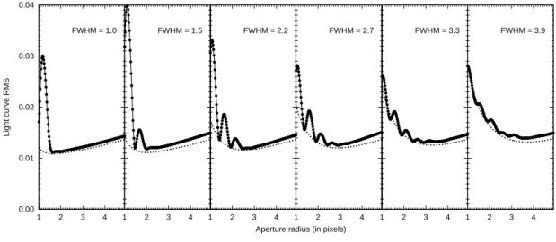
Figure 2.2: The graphs are showing the light curve scatters for mock stars (with 1% photon noise rms) when their flux is derived using aperture photometry. The subsequent panels shows the scatter for increasing stellar profile FWHM, assuming an aperture size between 1 and 5 pixels. The thick dots show the actual measured scatter while the dashed lines represent the lower limit of the light curve rms, derived from the photon noise and the background noise.

yields a non-negligible correlation between the raw and/or instrumental magnitudes and the fractional centroid positions. Advanced detectors such asback-illuminated CCD chips reduce the side effects of subpixel structure and also have larger quantum efficiency. Fig. 2.1 shows that the effect of the subpixel structure on the quality of the photometry highly dominates for sharp stars, where FWHM.1.2 pixels.

Spatial quantization and the size of the aperture

On CCD images, aperture photometry is the simplest technique to derive fluxes of individual point sources. Moreover, advanced methods such as photometry based on PSF fitting or image subtraction also involve aperture photometry on the fit residuals and the difference images, thus the properties of this basic method should be well understood. In principle, aperture is a certain region around a source. For nearly symmetric sources, this aperture is generally a circular region with a pre-defined radius. Since the image itself is quantized (i.e. the fluxes are known only for each pixel) at the boundary of the aperture, the per pixel flux must be properly weighted by the area of the intersection between the aperture and the pixel. Aperture photometry is implemented in almost all of the astronomical data reduction software packages (see e.g. Stetson, 1987). As it is known from the literature (Howell, 1989), both small and large apertures yield small signal-to-noise ratio (SNR) or relatively high light curve scatter (or root mean square, rms). Small aperture contains small amount of flux therefore Poisson noise dominates. For large apertures, the background noise reduces the SNR ratio. Of course, the size of the optimal aperture depends on the total flux of the source as well as on the magnitude of the background noise. For fainter sources, this optimal

(17)

0.0 0.5 1.0 1.5 2.0

0.0 0.5 1.0 1.5 2.0 2.5 3.0

RMS in # of intersecting square tiles

Radius

Figure 2.3: If circles with a fixed radius are drawn randomly and uniformly to a grid of squares, the number of intersecting squares has a well-defined scatter (since the number of squares intersecting the circle depends not only the radius of the circle but on the centroid position). The plot shows this scatter as the function of the radius.

aperture is smaller, approximately its radius is in the range of the profile FWHM, while for brighter stars it is few times larger than the FWHM (see also Howell, 1989). However, for very narrow/sharp sources, the above mentioned naive noise estimation becomes misleading.

As it is seen in the subsequent panels of Fig. 2.2, the actual light curve scatter is a non-trivial oscillating function of the aperture size and this oscillation reduces and becomes negligible only for stellar profiles wider than FWHM & 4.0 pixels. Moreover, a “bad” aperture can yield a light curve rms about 3 times higher than the expected for very narrow profiles.

The oscillation has a characteristic period of roughly 0.5 pixels. It is worth to mention that this dependence of the light curve scatter on the aperture radius is a direct consequence of the topology of intersecting circles and squares. Let us consider a bunch of circles with the same radius, drawn randomly to a grid of squares. The actual number of the squares that intersect a given circle depends on the circle centroid position. Therefore, if the circles are drawn uniformly, this number of intersecting squares has a well defined scatter. In Fig. 2.3 this scatter is plotted as the function of the circle radius. As it can be seen, this scatter oscillates with a period of nearly 0.5 pixels. Albeit this problem is much more simpler than the problem of light curve scatter discussed above, the function that describes the dependence of the scatter in the number of intersecting squares on the circle radius has the same qualitative behavior (with the same period and positions of local minima). This is an indication of a non-trivial source of noise presented in the light curves if the data reduction is performed (at least partially) using the method of aperture photometry. In the case of HATNet, the typical FWHM is between ∼ 2 −3 pixels. Thus the selection of a proper aperture in the case of simple and image subtraction based photometry is essential. The methods intended to reduce the effects of this quantization noise are going to be discussed later on, see Sec. 2.10.

(18)

-0.2 -0.1 0.0 0.1 0.2

5 10 15

0.0 0.2 0.4 0.6 0.8 1.0 0.0 0.2 0.4 0.6 0.8 1.0

FWHM = 0.95

5 10 15

FWHM = 1.30

5 10 15

FWHM = 1.89

5 10 15

FWHM = 2.83

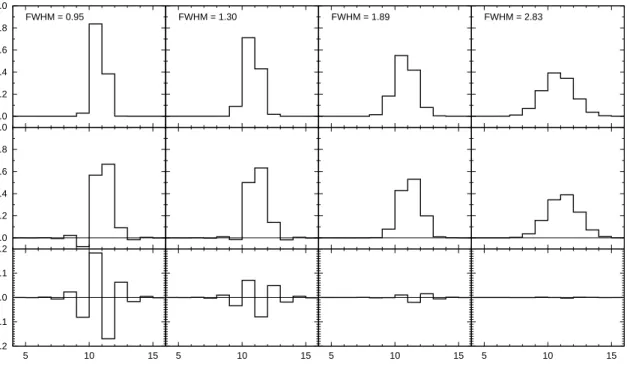
Figure 2.4: One-dimensional stellar profiles for various FWHMs, shifted using spline interpolation. The profiles on the upper stripe show the original profile while the plots in the middle stripe show the shifted ones. All of the profiles are Gaussian profiles (with the same total flux) and centered at x0 = 10.7. The shift is done rightwards with an amplitude of

∆x= 0.4. The plots in the lower stripe show the difference between the shifted profiles and a fiducial sampled profile centered atx=x0+ ∆x= 10.7 + 0.4 = 11.1.

Spline interpolation

As it is discussed later on, one of the relevant steps in the photometry based on image subtraction is the registration process, when the images to be analyzed are spatially shifted to the same reference system. As it is known, the most efficient way to perform such a registration is based on quadratic or cubic spline interpolations. Let us suppose a sharp structure (such as a narrow, undersampled stellar profile) that is shifted using a transformation aided by cubic spline interpolation. In Fig. 2.4 a series of one-dimensional sharp profiles are shown for various FWHMs between ∼ 1 and∼3 pixels, before and after the transformation. As it can be seen well, for very narrow stars, the resulted structure has values smaller than the baseline of the original profile. For extremely sharp (FWHM≈1) profiles, the magnitude of these undershoots can be as high as 10−15% of the peak intensity. Moreover, the difference between the shifted structure and a fiducial profile centered on the shifted position also has a specific oscillating structure. The magnitude of such oscillations decreases dramatically if the FWHM is increased. For profiles with FWHM ≈3, the amplitude of such oscillation is about a few thousandths of the peak intensity (of the original profile). If the photometry is performed by the technique of image subtraction, such effects yield systematics in the photometry. Attempts to reduce these effects are discussed later on (see Sec. 2.9).

(19)

0.5 1 1.5 2 2.5 3 3.5 4

FWHM (fitted)

FWHM (real)

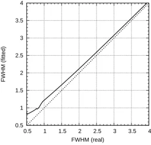
Figure 2.5: This plot shows how the profile FWHM is overestimated by the simplification of the fit. The continuous line shows the fitted FWHM if the model function is sampled at the pixel centers (instead of integrated properly on the pixels).

The dashed line shows the identity function, for comparison purposes.

Profile modelling

Regarding to undersampled images, one should mention some relevant details of profile modelling. In most of the data reduction processes, stellar profiles detected on CCD images are characterized by simple analytic model functions. These functions (such as Gaussian or Moffat function) have a few parameters that are related to the centroid position, peak intensity and the profile shape parameters. During the extraction of stellar sources the parameters of such model functions are adjusted to have a best fit solution for the profile.

In order to perform a self-consistent modelling, one should derive the integrated value of the model function to adjacent pixels and fit these integrals to the pixel values instead of sampling the model function on a square grid and fit these samples to the pixel values. Although the calculations of such integrals and its parametric derivatives³ are computationally expensive, neglecting this effect yields systematic offsets in the centroid positions and a systematic overestimation of the profile size (FWHM). Since the plate solution is based on the individual profile centroid coordinates, such simplification in the profile modelling yields additional systematics in the final light curves⁴ Moreover, precise profile modelling is essential in the reduction of the previously discussed spline interpolation side effect. As an example, in Fig. 2.5 we show how the fitted FWHM is overestimated by the ignorance of the proper profile modelling, if the profile model function is Gaussian.

3Parametric derivatives of the model functions are required by most of the fitting methods.

4For photometry, the final centroid positions are derived from the plate solution and a catalogue. There- fore, systematic variations in the plate solution indirectly yield systematic variations in the photometry and in the light curves.

(20)

2.1.2 Crowded images

Since the “CCD era”, various dense stellar fields, such as globular clusters or open clusters are monitored for generic photometric analysis and variability search. The main problems of such crowded images are well known and several attempts have been done in order to reduce the side effects resulted from the merging profiles. In this section some of the problems are discussed briefly.

Merging and sensitivity to profile sharpness

Merging of the adjacent stellar profiles have basically two consequences in the point of photometry. First, it is hard to derive the background intensity and noise level around a given target star. Stars in the background area can be excluded by two ways: the pixels belonging to such profiles can be ignored either by treating them outliers or the proximity of other photometric centroids are removed from the set of background pixels. The second consequence of the profile merging is the fact that flux from adjacent stars is likely to be

“flowed” underneath to the target aperture. Moreover, the magnitude of such additional flux depends extremely strongly on the profile FWHMs and therefore variations in the widths of the profiles cause significant increase in the light curve scatter.

Modelling

The modelling of stellar profiles, both by analytical model functions and empirical point- spread functions are definitely hardened in the case of merging sources. In this case the detected stars cannot be modelled separately, thus a joint fit should be performed simultaneously on all of the stars or at least on the ones that are relatively close to each other to have significant overlapping in the model functions. In the case of extremely crowded fields, sophisticated grouping and/or iterative procedures should be employed, otherwise the computation of the inverse matrices (associated with the parameter fitting) is not feasible (see also Stetson, 1987).

As we will see later on, the method of difference image photometry helps efficiently to reduce these side effects related to the crowdness of the images. However, it is true only for differential photometry, i.e. during the photometry of the reference frames⁵ these problems still emerge.

5In principle, the method of differential photometry derives the flux of objects on a target image by adding the flux of the objects on a reference image to the flux of the residual on the image calculacted as the difference between the target and the reference image.

(21)

2.1.3 Large field-of-view

Additionally to the previously discussed issues, the large size of the field-of-view also intro- duces various difficulties.

Background variations

Images covering large field-of-view on the sky are supposed to have various background structures, such as thin cirrus clouds, or scattered light due to dusk, dawn or the proximity of the Moon or even interstellar clouds⁶. These background variations make impossible the derivation of a generic background level. Moreover the background level cannot be characterized by simple functions such as polynomials or splines since it has no any specific scale length. Because the lack of a well-defined background level, the source extraction algorithm is required to be purely topological (see also Sec. 2.4).

Vignetting, signal-to-noise level and effective gain

The large field-of-view can only be achieved by fast focal ratio optical designs. Such optical systems do not have negligible vignetting, i.e. the effective sensitivity of the whole system decreases at the corners of the image. In the case of HATNet optics, such vignetting can be as strong as 1 to 10. Namely, the total incoming flux at the corners of the image can be as small as the tenth of the flux at the center of the image. Although flat-field corrections eliminate this vignetting, the signal-to-noise ratio is unchanged. Since the latter is determined by the electron count, increasing the flux level reduces the effectivegain⁷at the corner of the images.

Since the expectations of the photometric quality (light curve scatter and/or signal-to-noise) highly depends on this specific gain value, the information about this yield of vignetting should be propagated through the whole photometric process.

Astrometry

Distortions due to the large field-of-view affects the astrometry and the source identification.

Such distortions can efficiently be quantified with polynomial functions. After the sources are identified, the optimal polynomial degree (the order of the fit) can easily be obtained by calculating the unbiased fit residuals. For a sample series of HATNet images we computed these fit residuals, as it is shown in Table 2.1. It can easily be seen that the residuals do not

6Although interstellar clouds are steady background structures, in the point of the analysis of a single image, these cause the same kind of features on the image.

7The gain is defined as the joint electron/ADU conversion ratio of the amplifier and the A/D converter.

A certain CCD camera may have a variable gain if the amplification level of the signal read from the detector can be varied before digitization.

(22)

Table 2.1: Typical astrometric residuals in the function of polynomial transformation order, for absolute and relative transformations. For absolute transformations the reference is an external catalog while for relative transformations, the reference is one of the frames.

Order Absolute Relative 1 0.841−0.859 0.117−0.132 2 0.795−0.804 0.049−0.061 3 0.255−0.260 0.048−0.061 4 0.252−0.259 0.038−0.053 5 0.086−0.096 0.038−0.053 6 0.085−0.096 0.038−0.053 7 0.085−0.095 0.038−0.053 8 0.085−0.095 0.038−0.053 9 0.085−0.095 0.038−0.053

decrease significantly after the 5−6th order if an external catalogue is used as a reference, while the optimal polynomial degree is around ∼ 3−4 if one of the images is used as a reference. The complex problem of the astrometry is discussed in Sec. 2.5 in more detail.

Variations in the profile shape parameters

Fast focal ratio optical instruments have significant comatic aberrations. The comatic aberration yields not only elongated stellar profiles but the elongation parameters (as well as the FWHMs themselves) vary across the image. As it was demonstrated, many steps of a complete photometric reduction depends on the profile sizes and shapes, the proper derivation of the shape variations is also a relevant issue.

Summary

In this section we have summarized various influences of image undersampling, crowdness and large field-of-view that directly or indirectly affects the quality of the photometry. Although each of the distinct effects can be well quantified, in practice all of these occur simultaneously.

The lack of a complete and consistent software solution that would be capable to overcome these and further related problems lead us to start the development of a program designed for these specific problems.

In the next section we review the most wide-spread software solutions in the field of astronomical photometric data reduction.

(23)

Table 2.2: Comparison of some of the existing software solutions for astronomical image processing and data reduction. All of these software systems are available for the general public, however it does not mean automatically that the particular software is free or open source. This table focuses on the most wide-spread softwares, and we omit the “wrappers”, that otherwise allows the access of such programs from different environments (for instance, processing of astronomical images in IDL use IRAF as a back-end).

Pros Cons

IRAF¹

•Image Reduction and Analysis Facility. The most commonly recognized software for astronomical data reduction, with large literature and numerous references.

•IRAF supports the functionality of the package DAOPHOT², one of the most frequently used software solution for aperture photometry and PSF photometry with various fine-tune parameters.

•IRAF is a complete solution for image analysis, no additional software is required if the general functionality and built-in algorithms of IRAF (up to instrumental photometry) are sufficient for our demands.

•Not an open source software. Although the higher level modules and tasks are implemented in the own programming language of IRAF, the back-end programs have non-published source code. Therefore, many of the tasks and jobs are done by a kind of “black box”, with no real assumption about its actual implementation.

•Old-style user interface. The primary user interface of IRAF follows the archaic designs and concepts from the eighties. Moreover, many options and parameters reflect the hardware conditions at that time (for instance, reading and writing data from/to tapes, assuming very small memory size in which the images do not fit and so on).

•Lack of functionality required by the proper processing of wide-field images. For instance, there is no particular effective implementation for astrometry or for light curve processing (such as transposing photometric data to light curves and doing some sort of manipulation on the light curves, such as de-trending).

ISIS³.

•Image subtraction package. The first software solution employing image subtraction based photometry.

•The program performs all of the necessary steps related to the image subtraction algorithm itself and the photometry as well.

•Fully open source software, comes with some shell scripts (written in C shell), that demonstrate the usage of the program, as well as these scripts intend to perform the whole process (including image registration, a fit for convolution kernel and photometry).

•Not a complete software solution in a wider context. Additional software is required for image calibration, source detection and identification and also for the manipulation of the photometric results.

•Although this piece of software has open source codebase, the algo- rithmic details and some tricks related to the photometry on subtracted images are not documented (i.e. neither in the reference scientific arti- cles nor in the program itself).

•The kernel basis used by ISIS is fixed. The built-in basis involves a set of functions that can easily and successfully be applied on images with wider stellar profiles, but not efficient on images with narrow and/or undersampled profiles.

•Some intermediate data are stored in blobs. Such blobs may contain useful information for further processing (such as the kernel solution itself), but the access to these blobs is highly inconvenient.

SExtractor⁴.

•Source-Extractor. Widely used software package for extracting and classifying various kind of sources from astronomical images.

•Open source software.

•Ability to perform photometry on the detected sources.

•The primary goal of SExtractor was to be a package that focuses on source classification. Therefore, this package is not a complete solution for the general problem, it can be used only for certain steps of the whole data reduction.

•Photometry is also designed for extended sources.

1IRAF is distributed by the National Optical Astronomy Observatories, which are operated by the Association of Universities for Research in Astronomy, Inc., under cooperative agreement with the National Science Foundation. See alsohttp://iraf.net/.

2 DAOPHOT is a standalone photometry package, written by Peter Stetson at the Dominion Astrophysical Observatory (Stetson, 1987).

3ISIS is available fromhttp://www2.iap.fr/users/alard/package.html with additional tutorials and documentation (Alard

& Lupton, 1998; Alard, 2000).

4SExtractor is available fromhttp://sextractor.sourceforge.net/, see also Bertin & Arnouts (1996).

(24)

2.2 Problems with available software solutions

In the past decades, several software packages became available for the general public, intended to perform astronomical data reductions. The most widely recognized package is the Image Reduction and Analysis Facility (IRAF), distributed by the National Optical Astron- omy Observatories (NOAO). With the exception of photometry methods of image subtraction, many algorithms related to photometric data reductions have been implemented in the framework of IRAF (for instance, DAOPHOT, see e.g. Stetson, 1987, 1989). The first public implementation of the image convolution and the related photometry was given by Alard &

Lupton (1998), in the form of the ISIS package. This package is focusing on certain steps of the procedure but it is not a complete solution for data reduction (i.e. ISIS alone is not sufficient if one should derive light curves from raw CCD frames, in this case other packages must be involved due to the lack of several functionalities in the ISIS package). The SExtractor package of Bertin & Arnouts (1996) intends to search, classify and characterize sources of various kind of shape and brightness. This program was designed for extragalactic surveys, however, it has several built-in methods for photometry as well. Of course, there are several other independent packages or wrappers for the previously mentioned ones⁸. Table 2.2 gives a general overview of the advantages and disadvantages of the previously discussed software packages. Currently, one can say that these packages alone do not provide sufficient functionality for the complete and consistent photometric reduction of the HATNet frames. In the following, we are focusing on those particular problems that arise during the photometric reductions of images similar to the HATNet frames and as of this writing, do not have any publicly available software solutions to overcome.

2.3 Calibration and masking

For astronomical images acquired by CCD detectors, the aim of the calibration process is twofold. The first goal is to reduce the effect of both the differential light sensitivity characteristics of the pixels and the large-scale variations yielded by the telescope optics.

The second goal is to mark the pixels that must be excluded from the further data reduction since the previously mentioned corrections cannot be e performed because of various reasons.

The most common sources of such reasons are the saturation and blooming of bright pixels, cosmic ray events or malfunctioning pixels (such as pixels with highly nonlinear response or with extraordinary dark current). Of course, some of these effects vary from image to image (e.g. saturation or cosmic ray events) while other ones (such as nonlinear pixels) have

8These wrappers allow the user to access functionalities from external data processing environments. For instance, the astronomical reduction package of the IDL environment uses the IRAF as a back-end, or the package PyRAF provides access to IRAF tasks within the Python language.

(25)

2.3. CALIBRATION AND MASKING

constant structure.

In this section the process of the calibration is described, briefly discussing the sensitivity corrections, followed by a bit more detailed explanation of the masking procedure (since it is a relevant improvement comparing to the existing software solutions). Finally, we show how these masks are realized and stored in practice. The actual software implementation related to the calibration process are described later in Sec. 2.12.

2.3.1 Steps of the calibration process

Basically, the calibration of all of the image frames, almost independently from the instrumentation, has been done involving bias, dark and flat images and overscan correction (where an appropriate overscan section is available on the detector). These calibration steps correct for the light sensitivity inhomogeneities with the exception of nonlinear responses, effects due to the dependence on the spatial and/or temporal variations in the telescope position or in the sky background⁹ and second-order sensitivity effects¹⁰. In practice, the linear corrections provided by the classic calibration procedure are acceptable, as in the case of HATNet image calibrations.

Let us consider an imageI and denote its calibrated form by C(I). If the basic arithmetic operators between two images are defined asper pixel operations, C(I) can be derived as

C(I) = I−O(I)−B0 −(τ[I]/τ[D0])D0

F₀/kF₀k , (2.1)

where O(I) is the overscan level¹¹ of the imageI; B0, D0 and F0 are the master calibration images of bias, dark and flat, respectively. We denote the exposure time of the image x by τ[x]. kxk denotes the norm of the image x, that is simply the mean or median of the pixel values. In practice, when any of the above master calibration images does not exist in advance, one can substitute for these by zero, or in the case of flat images, by arbitrary positive constant value. The master calibration frames are the per pixel mean or median averages (with optionaln-σ rejection) of individual frames:

C(Bi) = Bi−O(Bi), (2.2)

B0 = hC(Bi)i, (2.3)

C(Di) = Di−O(Di)−B0, (2.4)

9Such as scattered light, multiple reflections in the optics or fringing yielded by the variations in the sky background spectrum

10such as the shutter effect

11Derived from the pixel values of the overscan area. The large scale structure of the overscan level is modelled by a simple function (such as spline or polynomial) and this function is then extrapolated to the image area.

(26)

D₀ = hC(D_i)i, (2.5) C(F_i) = F_i−O(F_i)−B₀− τ[F_i]

τ[D0]D₀, (2.6)

F0 = hC(Fi)i. (2.7)

Equations (2.2), (2.4) and (2.6) clearly show that during the calibration of the individual bias, dark and flat frames, only overscan correction, overscan correction and a master bias frame, and overscan correction, a master bias and a master dark frame are used, respectively.

2.3.2 Masking

As it was mentioned earlier, pixels having some undesirable properties must be masked in order to exclude them from further processing. The fi/fihat package and therefore the pipeline of the whole reduction supports various kind of masks. These masks are trans- parently stored in the image headers (using special keywords) and preserved even if an independent software modifies the image. Technically, this mask is a bit-wise combination of Boolean flags, assigned to various properties of the pixels. In this paragraph we briefly summarize our masking method.

First, before any further processing and right after the readout of the images, a mask is added to mark the bad pixels of the image. Bad pixels are not only hot pixels but pixels where the readout is highly nonlinear or the readout noise is definitely larger than the average for the given detector. These bad masks are determined after a couple of sky flats were acquired. Using sky flats for the estimation of nonlinearity and readout noise deviances are fairly good, since during dusk or dawn, images are exposed with different exposure times yielding approximately the same flux and all of the pixels have a locally uniform incoming flux. See Bakos (2004) for further details.

Second, all saturated pixels are marked with a saturation mask. In practice, there are two kind of effects related to the saturation: 1) when the pixel itself has an intensity that reaches the maximum expected ADU value or 2) if there is no support for anti-blooming in the detector, charges from saturated pixels can overflow into the adjacent ones during readout. These two types of saturation are distinguished in the oversaturation mask and blooming mask. If any of these mask are set, the pixel itself is treated as saturated. We note that this saturation masking procedure is also done before any calibration.

Third, after the calibration is done, additional masks can be added to mark the hot pixels (that were not corrected by subtracting the dark image), cosmic ray events and so on.

Actually, the latest version of the package supports the following masks:

• Mask for faulty pixels. These pixels show strong non-linearity. These masks are derived occasionally from the ratios of flat field images with low and high intensities.

(27)

2.3. CALIBRATION AND MASKING

• Mask for hot pixels. The mean dark current for these pixels is significantly higher than the dark current of normal pixels.

• Mask for cosmic rays. Cosmic rays cause sharp structures, these structures mostly resemble hot or bad pixels, but these does not have a fixed structure that is known in advance.

• Mask for outer pixels. After a geometric transformation (dilation, rotation, registration between two images), certain pixels near the edges of the frame have no corresponding pixels in the original frame. These pixels are masked as “outer” pixels.

• Mask for oversaturated pixels. These pixels have an ADU value that is above a certain limit defined near the maximum value of the A/D conversion (or below if the detector shows a general nonlinear response at higher signal levels).

• Mask for blooming. In the cases when the detector has no antiblooming feature or this feature is turned off, extremely saturated pixels causes “blooming” in certain directions (usually parallel to the readout direction). The A/D conversion value of the blooming pixels does not reach the maximum value of the A/D conversion, but these pixels also should be treated as somehow saturated. The “blooming” and “oversaturated” pixels are commonly referred as “saturated” pixels, i.e. the logical combination of these two respective masks indicates pixels that are related to the saturation and its side effects.

• Mask for interpolated pixels. Since the cosmic rays and hot pixels can be easily detected, in some cases it is worth to replace these pixels with an interpolated value derived from the neighboring pixels. However, these pixels should only be used with caution, therefore these are indicated by such a mask for the further processes.

We found that the above categories of 7 distinct masks are feasible for all kind of applications appearing in the data processing. The fact that there are 7 masks – all of which can be stored in a single bit for a given pixel – makes the implementation quite easy. All bits of the mask corresponding to a pixel fit in a byte and we still have an additional bit. It is rather convenient during the implementation of certain steps (e.g. the derivation of the blooming mask from the oversaturated mask), since there is a temporary storage space for a bit that can be used for arbitrary purpose.

2.3.3 Implementation

The basicper pixel arithmetic operations required by the calibration process are implemented in the programfiarith (see Sec. 2.12.2), while individual operations on associated masks can be performed using the fiign program (Sec. 2.12.6). Although the distinct steps of

(28)

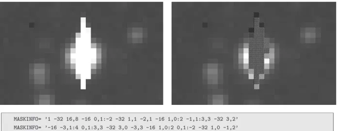
MASKINFO= ’1 -32 16,8 -16 0,1:-2 -32 1,1 -2,1 -16 1,0:2 -1,1:3,3 -32 3,2’

MASKINFO= ’-16 -3,1:4 0,1:3,3 -32 3,0 -3,3 -16 1,0:2 0,1:-2 -32 1,0 -1,2’

Figure 2.6: Stamp showing a typical saturated star. The images cover an approximately 8^′×5^′ area (32×20 pixels) of the sky, taken by one of the HATNet telescopes. The blooming structure can be seen well. The left panel shows the original image itself. In the right panel, oversaturated pixels (where the actual ADU values reach the maximum of the A/D converter) are marked with right-diagonal stripes while pixels affected by blooming are marked with left-diagonal stripes. Note that most of the oversaturated pixels are also blooming ones, since their lower and/or upper neighboring pixels are also oversaturated. Such pixels are therefore marked with both left- and right-diagonal stripes. Since the readout direction in this particular detector was vertical, the saturation/blooming structure is also vertical. The‘‘MASKINFO’’blocks seen below the two stamps show how this particular masking information is stored in the FITS headers in a form of special keywords.

Value Interpretation

T Use type T encoding. T = 0 implies absolute cursor movements, T = 1 implies relative cursor movements. Other values of T are reserved for optional further improvements.

−M Set the current bitmask toM. M must be between 1 and 127 and it is a bit-wise combination of the numbers 1, 2, 4, 8, 16, 32 and 64, for faulty, hot, cosmic, outer, oversaturated, blooming and interpolated pixels, respectively.

x, y Move the cursor to the position (x, y) (in the case of T = 0) or shift the cursor position by (x, y) (in the case ofT = 1) and mark the pixel with the mask value of M.

x, y:h Move/shift the cursor to/by (x, y) and mark the horizontal line having the length ofhand left endpoint at the actual position.

x, y:−v Move/shift the cursor to/by (x, y) and mark the vertical line having the length of v and lower endpoint at the actual position.

x, y:h, w Move/shift the cursor to/by (x, y) and mark the rectangle having a size of h×w and lower-left corner at the actual cursor position.

Figure 2.7: Interpretation of the tags foundMASKINFOkeywords in order to decode the respective mask. The values ofM,h, vandwmust be always positive.

the calibration can be performed by the appropriate subsequent invocation of the above two programs, a more efficient implementation is given by ficalib (Sec. 2.12.5), that allows fast evaluation of equation (2.1) on a large set of images. Moreover, ficalib also creates the appropriate masks upon request. The master calibration frames (referred as B0, D0

(29)

2.4. DETECTION OF STARS

and F₀ in equation 2.1) are created by the combination of the individual calibration images (see equations 2.3, 2.5 and 2.7), involving the program ficombine (Sec. 2.12.4). See also Sec. 2.12.5 for more specific examples about the application of these programs.

As it was mentioned earlier, the masks are stored in the FITS header using special keywords. Since pixels needed to be masked represent a little fraction of the total CCD area, only information (i.e. mask type and coordinates) about these masked pixels are written to the header. By default, all other pixels are “good”. A special form of run-length encoding is used to compress the mask itself, and the compressed mask is then represented by a series of integer numbers. This series of integers should be interpreted as follows.

Depending on the values of these numbers, a virtual “cursor” is moved along the image.

After each movement, the pixel under the cursor or a rectangle whose lower-left corner is at the current cursor position is masked accordingly. In Fig. 2.6 a certain example is shown demonstrating the masks in the case of a saturated star (from one of the HATNet images).

The respective encoded masks (as stored literally in the FITS header) can be seen below the image stamps. The encoding scheme is summarized in Fig. 2.7. We found that this type of encoding (and the related implementation) provides an efficient way of storing such masks.

Namely, the encoding and decoding requires negligible amount of computing time and the total information about the masking requires a few dozens from these “MASKINFO” keywords, i.e. the size of the FITS image files increases only by 3−5 kbytes (i.e. by less than 1%).

2.4 Detection of stars

Calibration of the images is followed by detection of stars. A successful detection of star-like objects is not only important because of the reduction of the data but for the telescopes of HATNet it is used in situ for guiding and slewing corrections.

In the typical field-of-view of a HATNet telescope there are 10⁴ – 10⁵ stars with suitable signal-to-noise ratio (SNR), which are proper candidates for photometry. Additionally, there are several hundreds of thousands, or millions of stars which are also easy to detect and characterize but not used for further photometry. The HATNet telescopes acquire images that are highly crowded and undersampled, due to the fast focal ratio instrumentation (f /1.8 for the lenses used by the HAT telescopes). Because of the large field-of-view, the sky background does also vary rapidly on an ordinary image frame, due to the large-scale structure of the Milky Way, atmospheric clouds, differential extinction or another light scattering effects.

Due to the fast focal ratio, the vignetting effects are also strong, yielding stars of the same magnitude to have different SNR in the center of the images and the corners. This focal ratio also results in stars with different shape parameters, i.e. systematically and heavily varying FWHM and elongation even for focused images (this effect is known ascomatic aberration